GNSS-R Observations of Marine Plastic Litter in a Water Flume: An Experimental Study

Abstract

Currently, eight million metric tons of plastic end up in the oceans every year, and microplastics in different forms are present in almost all water systems in the world: streams, rivers, lakes, or oceans, and even in our blood. Detection of marine litter is an urgent task. Some works have recently reported the potential of GNSS-Reflectometry to detect marine plastic litter from space. This study presents the results of a controlled field experiment conducted under the auspices of ESA at the “Atlantic Basin” at the Deltares research institute (Delft, The Netherlands). Several types of wave conditions were created: sinusoidal and with JONSWAP spectrum, with different significant wave heights, and with different types of plastics and marine litter collected from the Dutch coast. Experimental results show the difficulty in detecting marine plastic litter based on a change of the reflected power. However, a statistical analysis of the GNSS-R estimated reflectivities (amplitude and phase) computed with very short integration times (coherent integration time T_coh = 1 ms, and no incoherent averaging: N_incoh = 1) show that it may be possible to detect large accumulations of some types of marine litter that dampen the water waves, such as nets, bottles in a net, food wraps, and bags.

1. Introduction

As part of the “Global Monitoring of Microplastics using GNSS-Reflectometry” (GLIMPS) project led by Deimos Space UK, the Universitat Politècnica de Catalunya conducted a ground-based GNSS-R experiment in a controlled water flume: the “Atlantic Basin” at Deltares’ research premises (Delft, The Netherlands) under different wave conditions, and with different plastic types and concentrations.

Some works have recently reported the potential of GNSS-Reflectometry to detect marine plastic litter [1]. Although it is highly unlikely that at the GNSS L1 frequency the change in the dielectric constant could produce a detectable effect in the received signal through a change in the reflection coefficient, the presence of the plastics themselves could produce a detectable effect through a change in the surface roughness, either by damping the longer waves, or even by creating new capillary waves (“ripples”) when the wavefronts are distorted by the presence of the floating litter. This effect will likely be largely dependent on the size of the plastics used in the experiment, the wave’s characteristics, and the geometry of observation. These effects have been the object of the controlled empirical study presented in this work, with the main limitation (or advantage) being that the spatial resolution is given by the size of the first Fresnel zone, because of the dominant coherent scattering conditions [2,3].

In an open ocean scenario, the high bistatic reflectivity signatures observed in CYGNSS GNSS-R data may not be only due to the presence of the microplastics themselves. There is evidence that, for example, low surface roughness areas are linked to the presence of phytoplankton on the ocean surface [4]. It is likely that the biofouling or accumulation of microorganisms, plants, or algae on the plastics’ surfaces increases the concentration of surfactants, resulting in an increase of the wave damping. As plastics tend to accumulate in ocean current gyres, so do other surfactants and biofouling.

All these effects: (1) different surface roughness in the gyres regardless of the presence or not of plastics (or even in a hurricane eye in an extreme case, e.g., Figure 1 in [5]); (2) presence of phytoplankton and associated increased wave damping [4]; and (3) presence of plastics damping large waves [1], but possibly creating new ripples, have to be evaluated to assess the feasibility of detecting marine plastic litter from space. In this controlled experiment in a water flume, the third item is addressed.

This study describes the experiments conducted at the Atlantic Basin of the Deltares research institute (Delft, The Netherlands), during October 2021 [6]. It also describes the data processing, and the main conclusions, and it is structured as follows:

• Section 2 contains a detailed explanation of the materials and methods: the experiment’s setup, environment conditions (i.e., waves conditions and plastic types used),
• Section 3 presents the experimental results,
• Section 4 discusses the main results,
• Section 5 summarizes the main conclusions.

2. Materials and Methods

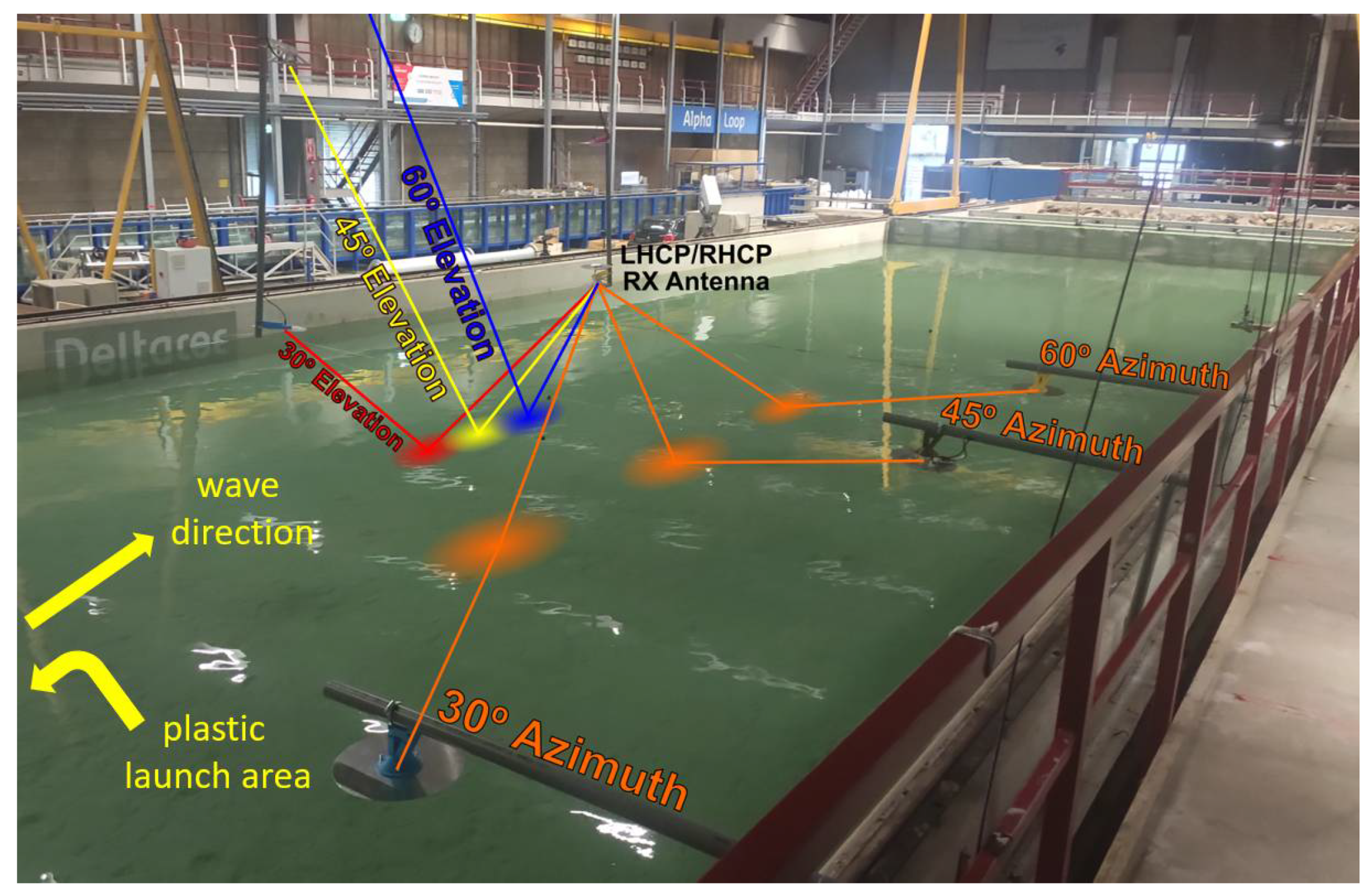
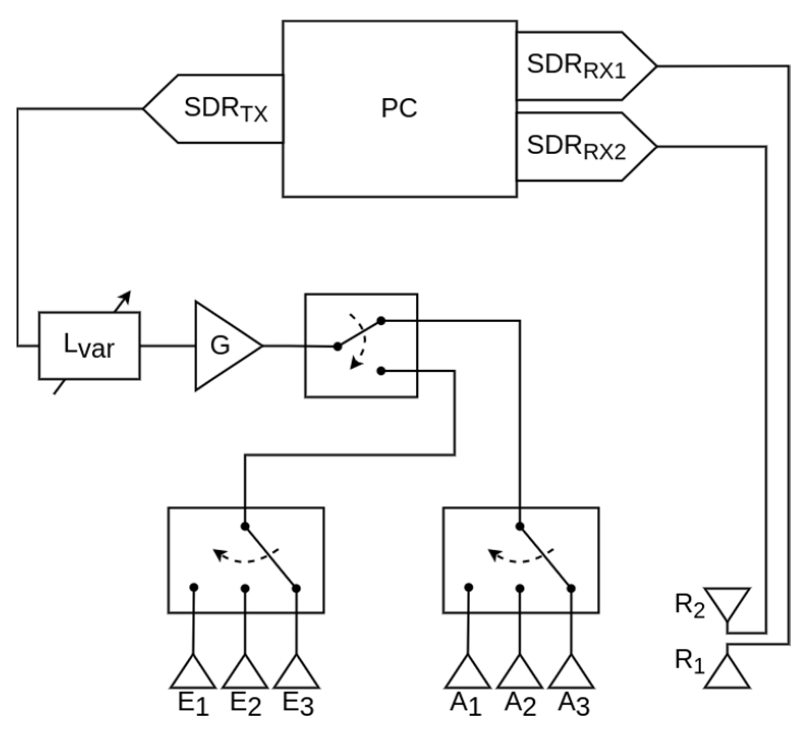
In order to explore new possibilities of GNSS-R systems such as different polarizations, complex (amplitude and phase information) reflection coefficients, shorter integration times, and/or statistical analysis of the observables, a GNSS-R-like system was developed by UPC which included on the reception side a dual-polarization (left and right hand circular polarizations, or, in short, LHCP and RHCP) down-looking antenna to pick the reflected GNSS signals, and a RHCP up-looking antenna to pick the direct signal. On the transmission side, several RHCP down-looking antennas created 3 different elevation angles (30°, 45°, and 60°) at azimuth 0°, and 3 different azimuth angles (30°, 45°, and 60°) at an elevation of 30°. In this study, only the azimuth 0° results are presented. The study included the analysis of the received signal intensity at both polarizations (LHCP and RHCP) looking for polarimetric signatures, and/or the instantaneous phase difference between them.

The following sections describe the GNSS-R system, and the experiment in detail.

2.1. GNSS-R-Like System

2.1.1. Transmission System

During the preparatory activities of the experiment, a GPS-like signal was generated at L1-band (1575.42 MHz) using a Rohde & Schwarz SMU-200A vector signal generator at UPC premises. The signal included the Coarse/Acquisition (C/A) Pseudo-Random Noise (PRN) codes 16, 20, 29, and 31 simultaneously, and the navigation information, which allowed to test the signal transmission in situ using a commercial GNSS receiver. Its power level was −81 dBm so that, with such a high SNR, the GNSS-R observables could be measured with very short integration times (coherent integration time T_coh = 1 ms, and no incoherent averaging: N_incoh = 1). This signal was recorded, and then played back using an ADALM-PLUTO (rev B) commercial off-the-shelf (COTS) software-defined radio (SDR) from analog devices [7].

Moreover, to track any frequency offset and drifts, at the beginning and at the end of each GPS-like signal, a CW beacon centered at L1-band + 500 kHz was also transmitted. Thus, the final synthesized transmitted signal consisted of 20 s of a synchronization CW beacon, followed by 40 s of an L1-band GPS signal, and finally 20 s of the synchronization CW beacon.

The signal was transmitted separately, and sequentially, by 6 different antennas. Three of them were located at an azimuth angle of 0° with respect to the receiving antennas, at specific heights in order to have elevation angles of 60°, 45°, and 30°. The other three transmitting antennas were located at the same height, and at different azimuths of 60°, 45°, and 30° between the transmitters and the receivers (Figure 1). As will become evident, this is an important fact since, due to the small area that the system is getting the reflections, at a given time the footprints on the water surface are different. It is also worth noting that all the antennas were hanging from the 8.5 m height corridors, to avoid placing the masts and poles in the middle of the flume, which would have distorted the wave field.

A RF switching matrix controlled by a Raspberry Pi was used to perform the sequential sweep of the transmitting antennas. The transmitted signal was conditioned by means of a variable attenuator, and a fixed amplifier (Figure 2), to compensate the different signal path losses from each transmitting antenna, and to ensure a proper reception of the GPS signal. The variable attenuator was adjusted for each transmitter to achieve a CN0 from 35 dBHz to 50 dBHz, as measured with a commercial off the shelf (COTS) GPS receiver connected to the receiver’s side.

2.1.2. Reception System

The transmitted signal was then simultaneously received by two antennas placed at a 1 m height with respect to the water level: a RHCP one looking upwards to acquire the direct GPS signal, and a dual polarization one (RHCP and LHCP) looking downwards to pick the GPS signal scattered on the water surface.

The up-looking antenna was connected to a Universal Software Radio Peripheral (USRP) model B200mini-i from Ettus Research [8], which down-converted and sampled the received signal at a rate of f_s = 2.5 MSps. This signal is used as the reference one.

The down-looking antenna was connected to an ADALM-PLUTO (rev C) SDR [7], which down-converted and sampled synchronously the two received signals at both polarizations at a rate of f_s = 2.046 MSps.

2.1.3. Antennas Specifications

All the antennas were commercially available microstrip patch antennas. The transmission antennas for 30° and 60° elevation and azimuth angles, as well as the up-looking receiving antenna were RHCP matched at L1 and L5 GPS bands, with an axial ratio of ~2 dB, which were manufactured by Matterwaves Antenna Technology [9]. The 45° elevation and azimuth angles antennas as well as the down-looking antenna were L1 RHCP/LHCP dual-polarization antennas designed and manufactured in-house [10]. The main specifications are summarized in

Table 1. Antennas’ specifications.

		Angle [°]	Frequency [MHz]	Polarization
TX antennas	Elevation	30	1540–1610	RHCP
		45	1490–1700	RHCP/LCHP
		60	1540–1610	RHCP
	Azimuth	30	1540–1610	RHCP
		45	1530–1580	RHCP/LHCP
		60	1540–1610	RHCP
RX antennas	Up-looking		1540–1610	RHCP
	Down-looking		1500–1600	RHCP/LHCP

.

2.1.4. Reflection Geometry

A key aspect of the GNSS-R experiment implemented at Deltares premises was the location of the transmitting antennas to achieve different incidence angles to study the sensitivity of GNSS-R signals to the presence of surface plastics.

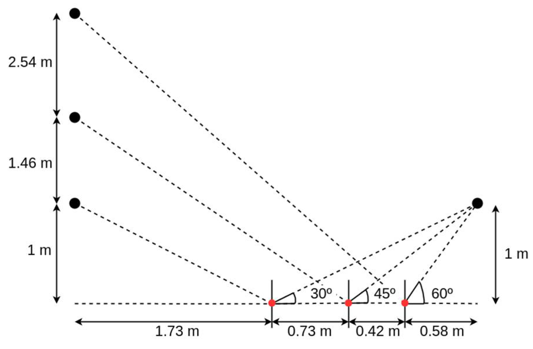
As it can be seen in Figure 3, the longitudinal separation between the mast holding the receiving antennas was 3.46 m. Since the receiving antennas were at 1 m height, the height of the elevation antennas to achieve reflection angles of 30°, 45°, and 60° in elevation were 1 m, 2.46 m, and 5 m, respectively. To achieve azimuthal angles of 30°, 45°, and 60°, the longitudinal separation of the transmitting antennas with respect to the receivers were 7.52 m, 4.34 m, 2.50 m, respectively.

Because of the small distances involved, the reflected signal comes from a small area that in many cases does not even include a single “long” wave period. Therefore, as will be evidenced later, a strong coherent component is expected. When a coherent reflection occurs, the area from which the signals are coming from is given by the so-called “first Fresnel zone” [2,3]. The first Fresnel zone is the ellipsoidal area surrounding the specular point where the path difference with respect the specular point is less than half wavelength ($\mathsf{\Delta }r\le \raisebox{1ex}{$\mathsf{\lambda }$}\!\left/ \!\raisebox{-1ex}{$2$}\right.$), or less than a phase shift of $\mathsf{\Delta }\mathsf{\varphi }\le 180°$:

$$R_1=\sqrt{\lambda ·\frac{D_{10}·D_{20}}{D_{10}+D_{20}}}, R_2=\frac{R_1}{sin{\theta }_{el}},$$

(1)

where R₁ is the radius of the first Fresnel zone, and R₂ is its projection (i.e., R₁ and R₂ are the semi-axes of the ellipse), λ is the electromagnetic wavelength, D₁₀ is the distance between the transmitter and the specular point, D₂₀ is the distance between the receiver and the specular point, and θ_el is the local elevation angle.

From the distances between the transmitters and the receivers, the radii of the first Fresnel zone are calculated and shown in

Table 2. First Fresnel zones specifications.

	Angle [°]	D10 [m]	D20 [m]	R1 [m]
Elevation	30	2.00	2.00	0.87
	45	3.48	1.41	0.62
	60	5.77	1.16	0.49
Azimuth (Elevation angle = 30°)	30	5.02	5.02	1.38
	45	3.55	3.55	1.16
	60	2.90	2.90	1.05

.

Antenna pattern sphericity effects are analyzed in [11]. Since the distance from the transmitting antenna to the specular reflection point is larger than the width of the first Fresnel zone. Therefore, the subtended angle is small enough so that the plane wave assumption approximately holds.

To ensure the presence of plastics inside the first Fresnel zone, during the execution of some particular tests, plastics had to be attached with the help of a thin nylon rope and placed inside this area. In the other tests, the plastic litter entered and left the Fresnel zone pushed by the waves, so it was only visible for a small fraction of the time. Note that for the lateral antennas (azimuth angles of 30°, 45°, and 60°) the number of events of plastic litter entering in their respective Fresnel zones was too small to allow to conduct the study.

2.2. Generation of Waves in the Tank

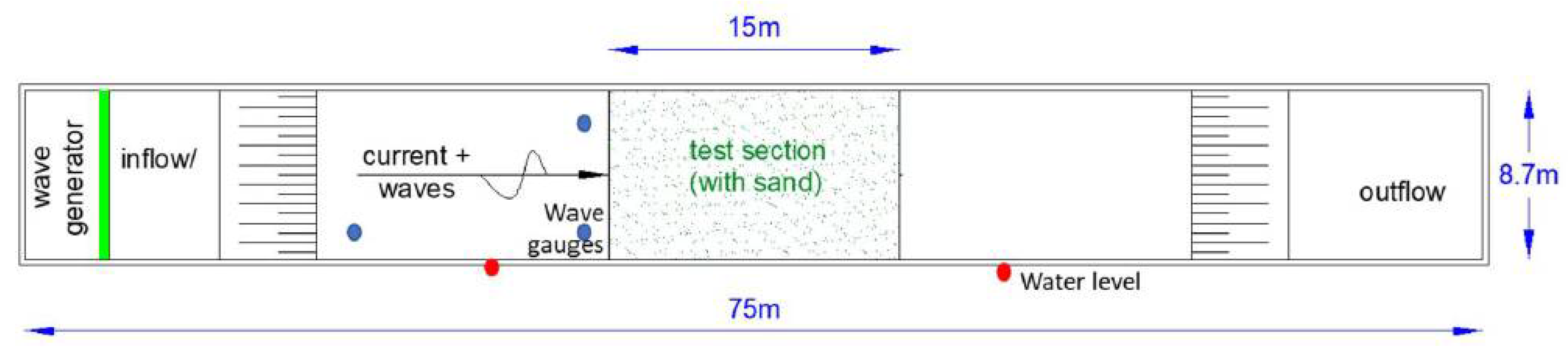
During the data acquisition, two independent environmental parameters were changed. The first one was related to the waves that were generated, while the second one referred to the kind of plastics thrown into the flume. The Deltares Atlantic Basin [12] flume at Delft, the Netherlands is 75 m long and 8.7 m wide, as shown in Figure 4.

Two different wave spectra were generated: (1) regular waves describing a periodic sinusoidal shape (or as close as possible to it) with a fundamental frequency of 0.833 Hz, and (2) irregular waves with a JONSWAP spectrum [13]. This wave spectrum relies on the data collected during the Joint North Sea Wave Observation Project, and was chosen to represent ocean wave conditions [13].

Four different amplitudes (5, 9, 12, and 17 cm) were generated using mechanical pedals on the left side of Figure 1 and Figure 4, and in selected cases, capillary waves were also generated on top of the long waves by means of a fan. Figure 5 shows several JONSWAP spectra realizations with a significant wave height of 9 cm, as measured by the wave gauges in the tank.

Moreover, capillary waves were also generated on top of the long waves by means of a fan, as they are weaker and easier to be dampened. Finally, distinct wave amplitudes were generated.

2.3. Plastic Litter

Multiple types of plastics are found in the oceans. In [14,15] it was shown that the most important polymer in terms of relative abundance in all the environment compartments, including marine and freshwater systems is polyethylene (HDPE and LDPE), followed by polypropylene (PP) and polystyrene (PS). Lebreton et al. [16] classified the ocean plastics in hard plastics, sheets and films (type H), ropes and fish nets (type N), pellets (type P), and foam (type F), and provided mass concentrations for these types of plastics where the plastic types N and H were most frequently observed in the Pacific gyre.

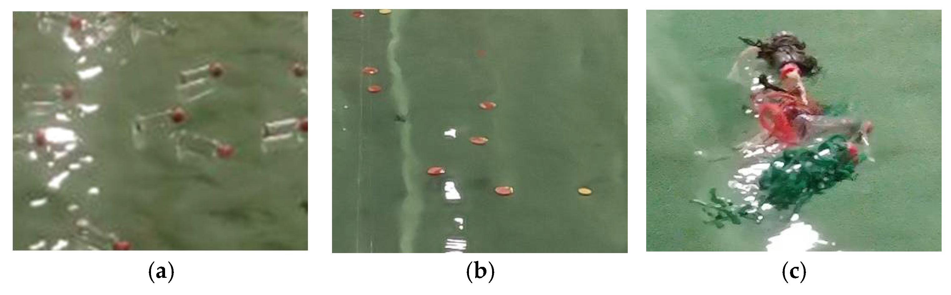
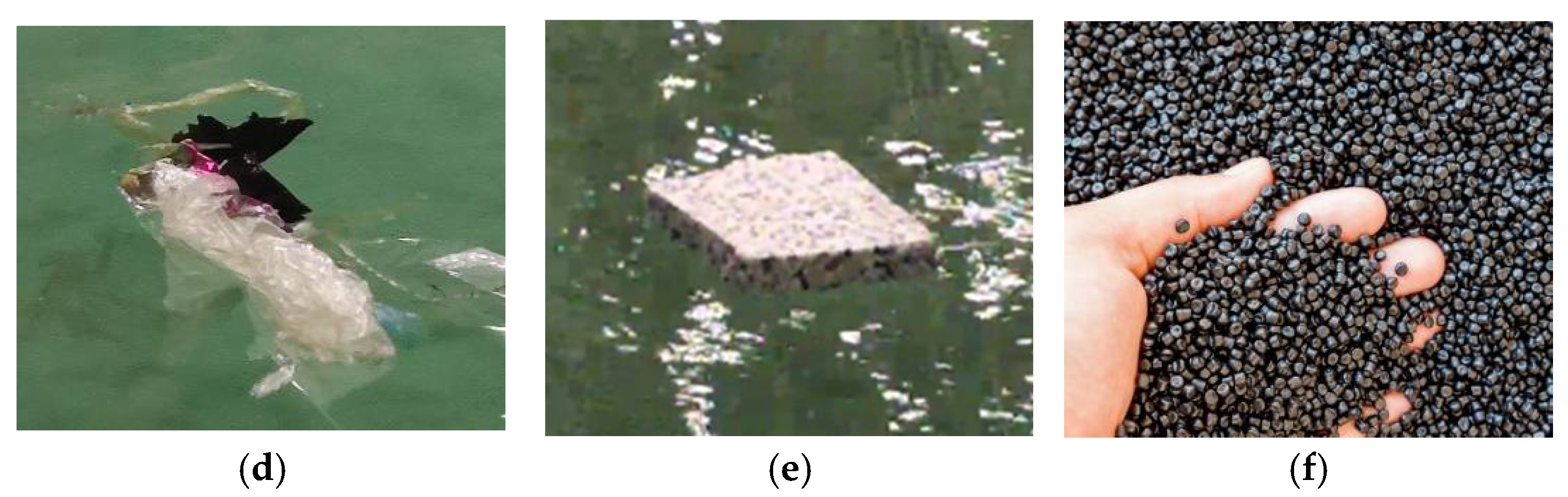
Plastics of different shapes, sizes, and types were used in this field experiment, in different concentrations to assess the impact of their presence in the water surface in the GNSS-R signal. The plastics used in these tests are both clean, newly produced plastics, as well as marine plastics collected in nature. The plastics used were: water bottles, bottle caps, fishing nets, marine litter bags, Styrofoam, polyethylene and polypropylene pellets. In total, 23 different types of plastics were used, some of them are shown in Figure 6.

Table 3. Plastics type (see text for description), concentration, surface density, and size, and wave conditions of the experiment (ϕ indicates diameter).

summarizes the experiment conditions: plastic types, concentration, surface density and size, and the rms wave height created with the mechanical paddles.

3. Results

A total of 123 potentially valid data files have been analyzed. As explained before, the high carrier-to-noise ratio (CN0) allows for the use of a coherent integration time as short as T_coh = 1 ms, without any incoherent averaging (N_inc = 1), which means that GNSS-R signals at 1 ms sampling rate could be analyzed.

During the experiments, the relative calibration between the reflected and the direct signals was first performed using the calm water as a reference (i.e., the known reflection coefficient at LHCP and RHCP for a given frequency, incidence angle, water temperature and salinity). Since the measured changes were very small, a differential analysis was conducted. In some occasions, the reference observation was not directly acquired immediately before, or even if it was, the surrounding conditions were not exactly the same (e.g., variable multipath as people moved around). This translated into fluctuations of the direct signal that were used to monitor the data quality.

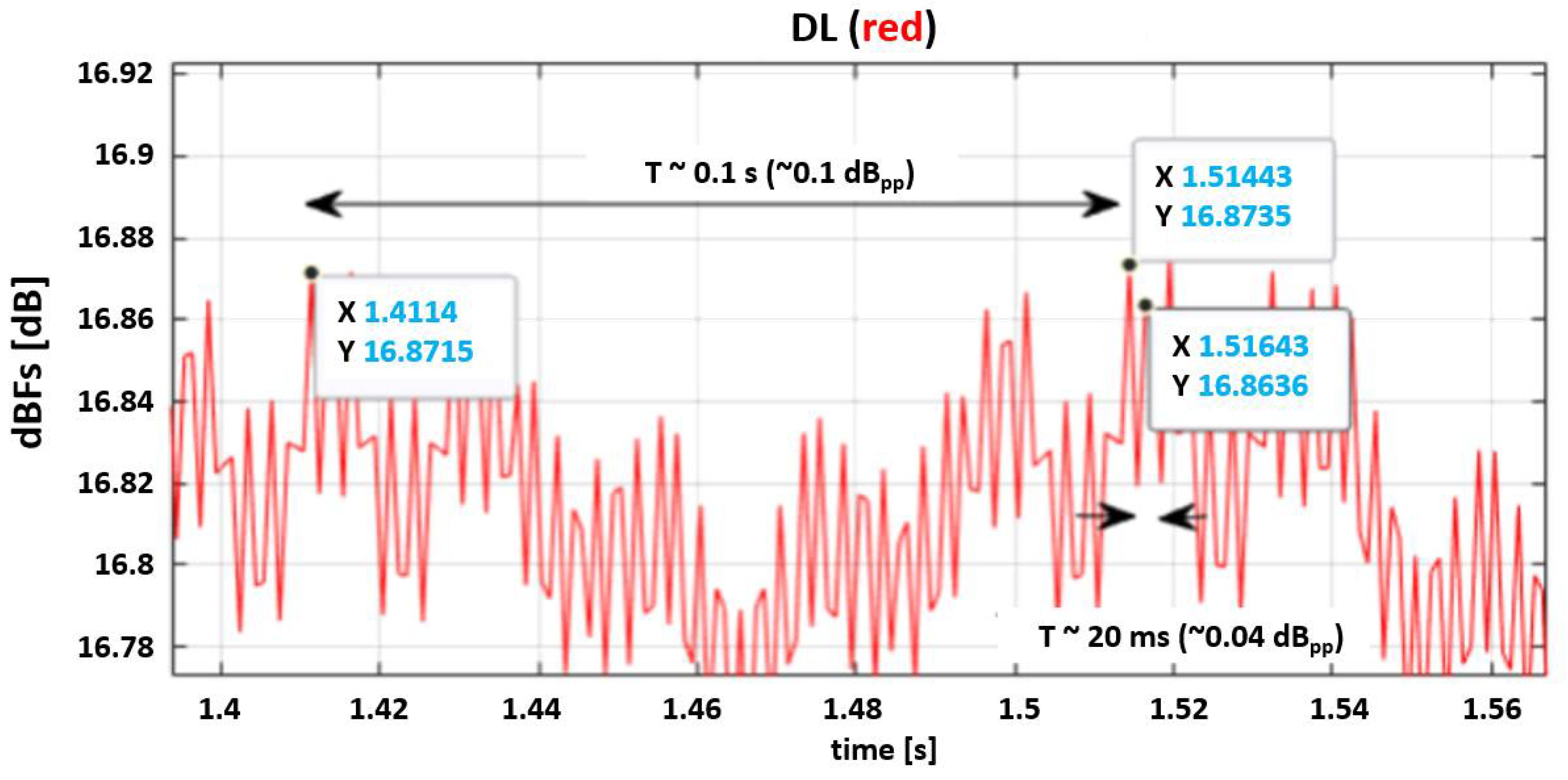
There are other examples where radio frequency interference (RFI) was very obvious, and these measurements had to be discarded as well. Some of the problems encountered include multipath in the direct signal (up-looking antenna) as well as RFI in the reflected signals (down-looking antennas), or fast electromagnetic interference (EMI with a period of T = 20 ms, f = 50 Hz) probably from power lines, although of very small amplitude (~0.04 dBpp), which can be neglected for all purposes (Figure 7). A second ripple of period T = 0.1 s (i.e., 10 Hz) with an amplitude of ~0.1 dBpp is also noticed, which seemed to be linked to small waves propagating in the water surface despite the fact that the mechanical pedals had been turned off for a while. This is normal, as for a very large basin like the Atlantic Basin, it is not possible to have a perfectly flat surface. Bad quality or corrupted data were discarded. The minimum detectable changes in Figure 7 set the limit of the smallest signature that can be detected (~0.04 dB).

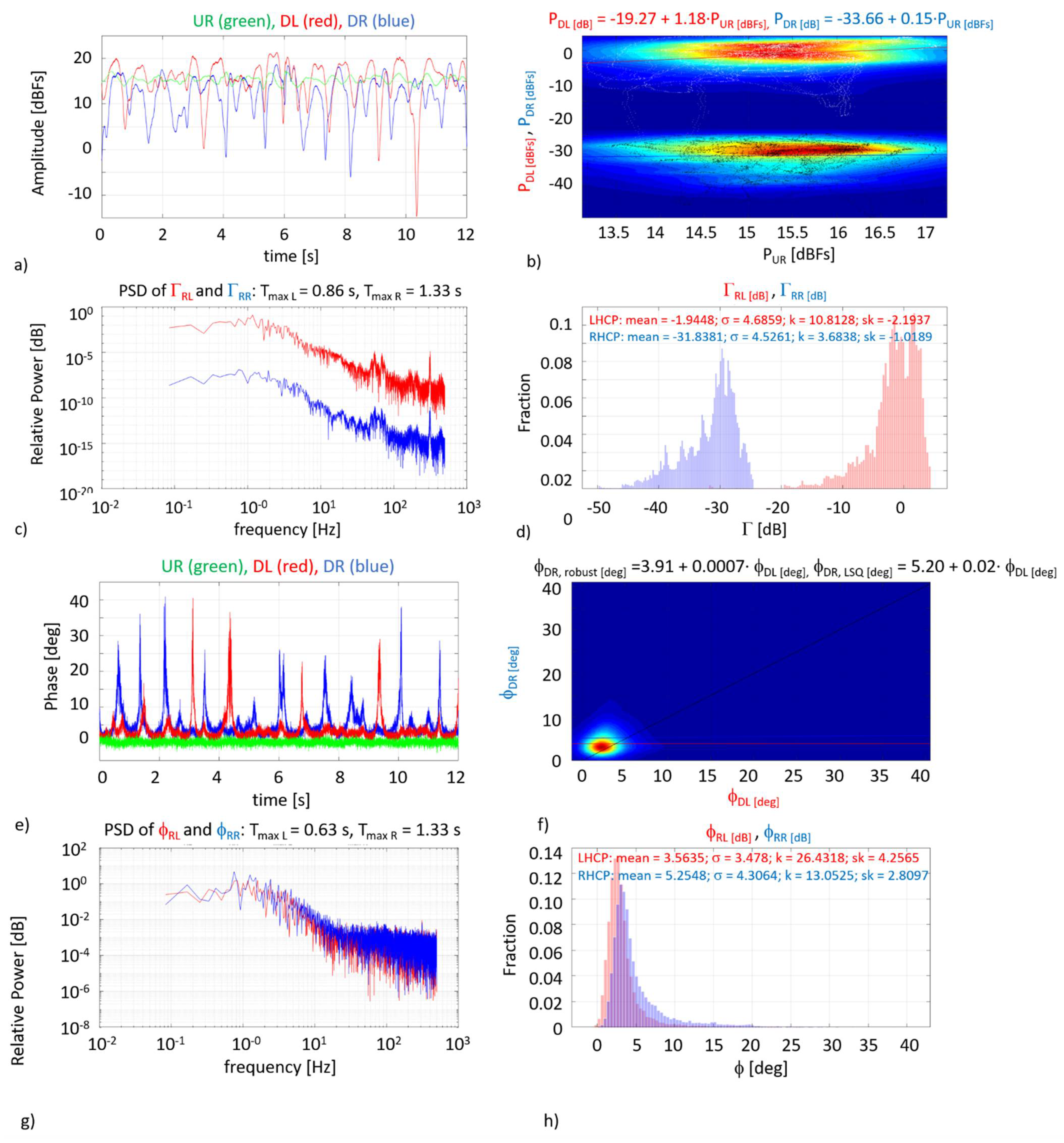
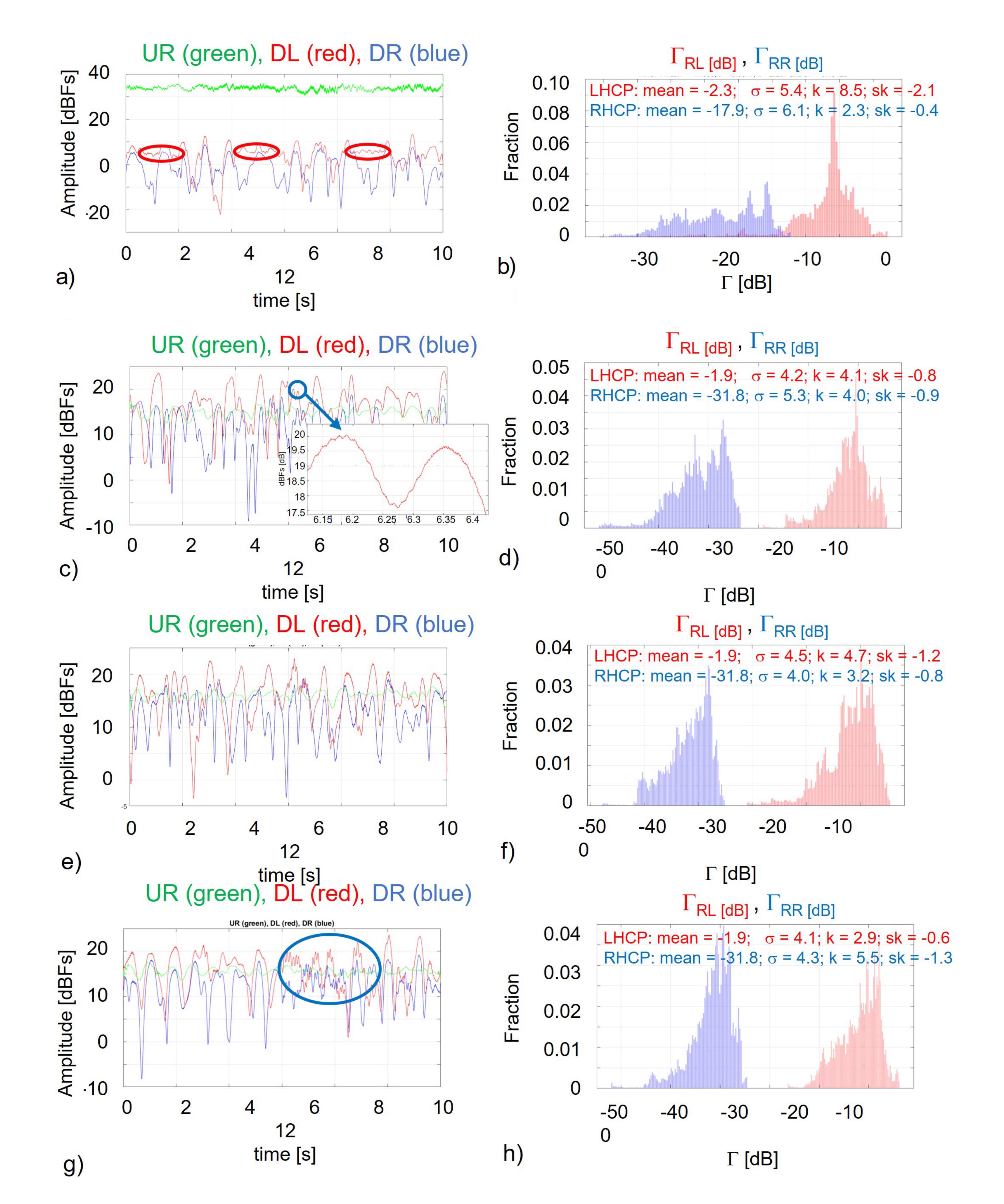
The analysis performed for each scenario includes (e.g., Figure 8 for clean rough water surface without capillary waves):

• For the amplitude (power): (a) time series, (b) multi-path quality check: scatter plot of received power at left (RL) and right (RR) polarizations in dB full scale (dBFs) versus the direct signal power also in dBFs, (c) spectra, (d) histogram of the received power at RL and RR polarizations;
• For the phase: (e) time series, (f) scatter plot of the phases at RR versus RL polarizations, (g) spectra, (h) histogram of the received phases at RL and RR polarizations.

Statistical descriptors are the mean, the standard deviation (σ), the kurtosis (k), and the skewness (sk).

Recall that the RL polarization is defined as incident wave at RHCP, and the reflected one at LHCP, and RR polarization as defined as incident wave at RHCP, and the reflected one at RHCP.

Time series (Figure 8a,e plots) allow for the gathering of an insight of the power or phase variations, which are very noticeable in the cases when the water surface is roughened. Also, the shape is different depending on the spectrum (i.e., sinusoidal vs. JONSWAP). While for a flat surface the received power is nearly constant and the phase has a Gaussian distribution, as it is just noise (not shown), for a roughened water surface, the received signal has a particular amplitude (Figure 8d) and phase (Figure 8h) distributions. The spectral analysis (e.g., Figure 8c) reveals a peak at the dominant wave period (e.g., ~0.86 s, or ~1.2–1.3 s in most cases), as shown in Figure 5. Peaks in the spectrum above ~10–20 Hz cannot be attributed to capillary waves, and they can only be attributed to electromagnetic interference. The same behavior occurs for the phase.

Since most of the changes are marginal and difficult to be observed with the naked eye (except in very few occasions), a statistical analysis is performed both for the amplitude (Figure 8d) and phase (Figure 8h) of the reflection coefficients, and four statistical descriptors are computed: mean value, standard deviation, kurtosis and skewness. It is worth noting that most of the changes observed occur in the standard deviation and/or in the kurtosis of the observable (amplitude or phase), and this is very clear in some selected cases in the histograms, especially as a function of the rms wave height, and its damping.

Also, as a multi-path quality check, a density plot overlaid with a scatter plot with the uncalibrated direct signal in the x-axis (dBFs: dB full scale), and the calibrated reflectivity in the y-axis (dB) is presented in the b plots. In an ideal scenario the direct signal power should be constant (i.e., multi-path free), the scatter plot should be a vertical line showing the variability of the received power when the direct signal is constant, but actually, it is not completely. As said, these figures are a sanity check of the quality of the data. For example, in Figure 8b, the error induced by the direct signal in the reflected signal powers is estimated to be (robustfit of the scatter plots, Figure 8b) ~1.18 dBFs/dBFs at RL, and ~0.15 dBFs/dBFs at RR, which are negligible as compared to the variations of the received power (red and blue lines fluctuations wrt. green line, Figure 8a).

The density plot of the phase (scatter plot not overlaid on top of it for clarity), Figure 8f must be interpreted as the correlation of the reflection coefficients at both polarizations which is linked to the instantaneous variations of the scattering coefficients at RL and RR polarizations.

Ten different case studies are presented: (1) Clean Flat and Roughened Water Surface With/Without Capillary Waves, (2) Clean Water–Variation with Incidence Angle, (3) Bottles and Fixed Net, (4) Plastic Bottles, (5) Marine Litter (Nets), (6) Marine Litter (Food Wraps and Bags), (7) Marine Litter (Caps and Lids), (8) Straws, (9) Pellets, and (10) Styrofoam.

These results are representative results for each case study, as in most cases, the experiment was repeated for consistency. In the following sections, the observables for a clean water surface, with/without waves/capillary waves are presented as the reference cases. Then, the results for the eight types of marine plastics are presented. Finally, Section 4 summarizes and discusses the average results for the different realizations performed.

3.1. Clean Roughened Water Surface with and without Capillary Waves

Figure 8 and Figure 9 show the results for clean roughened water surfaces for 30° elevation angle, with and without capillary waves.

In Figure 8 the sea surface follows the JONSWAP spectrum with a rms height of 5 cm. The time series of the RL and RR reflected signals exhibit a sharp periodic fading associated to the water surface waves, and the PSD shows a peak at T = 0.86 s, in agreement with the measured sea surface spectrum (Figure 5). Direct signal multi-path impact (Figure 8a, green line) is marginal as compared to the fluctuations of the RL and RR reflected signals (Figure 8b). Peaks above 50 Hz are due to EMI (Figure 8c). The PDF of the amplitude reflection coefficients (in dB) approximates to a log-normal (x-reversed and shifted, Figure 8d). Phase temporal series also show peaks (Figure 8e), but interestingly they are not correlated between polarizations, and histograms (Figure 8h) depart from a Gaussian shape observed in the flat surface case (not shown), and has a PDF reminiscent of a Rayleigh one.

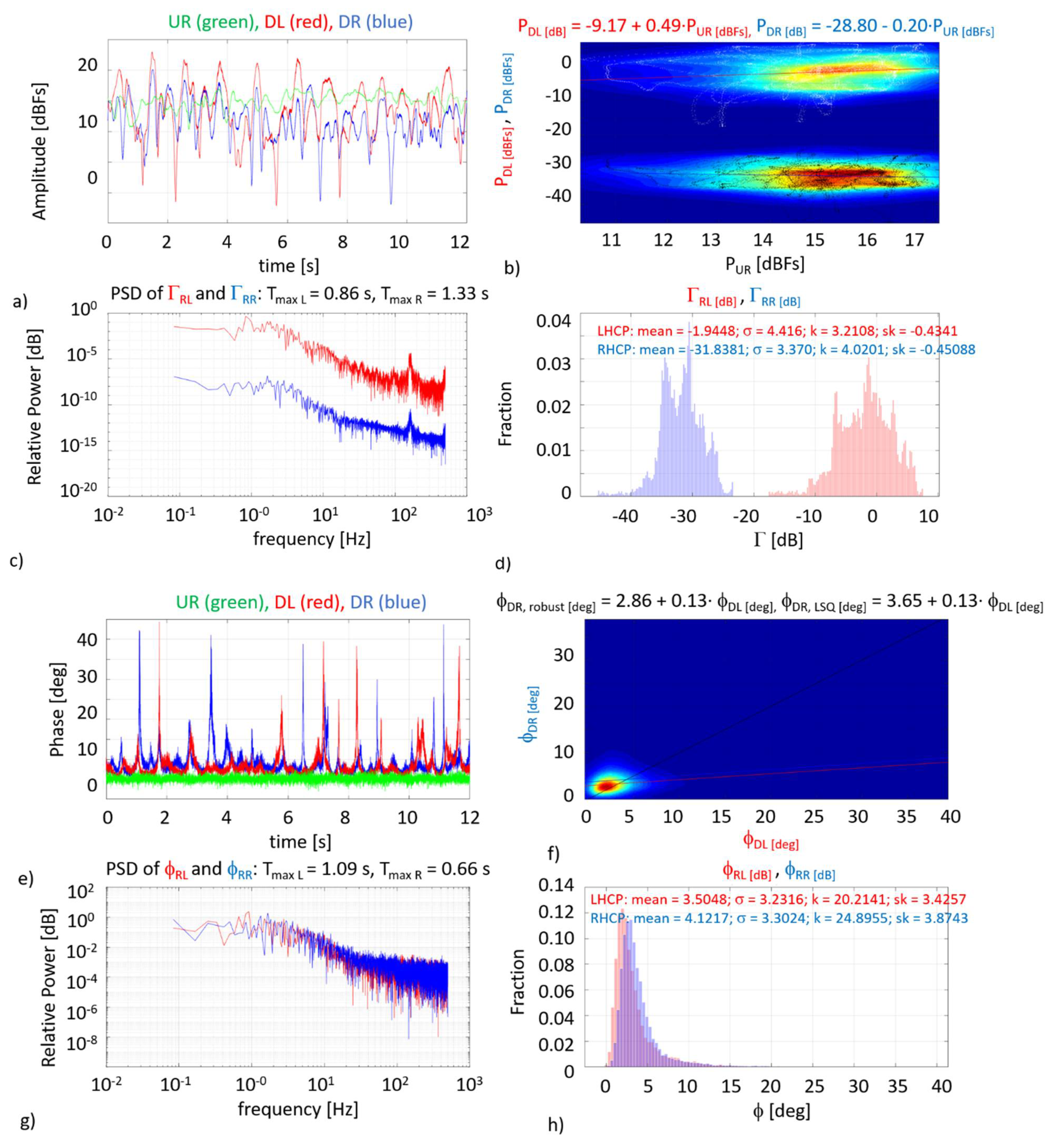
The impact of capillary waves is analyzed in the following figures. As in the previous figures, Figure 9 shows for clean roughed water surface and a significant wave height = 5 cm with capillary waves, and an elevation angle of 30° the time evolution (Figure 9a), the multi-path sanity check (Figure 9b), and the spectra (Figure 9c). In Figure 9c, a secondary peak (~200 Hz) appears, which can be attributed to EMI. The PDF of the reflection coefficients (Figure 9d) is “flattened” with respect to Figure 8d (no capillary waves case); its excursion is the nearly the same, and both the kurtosis and the skewness have notably decreased.

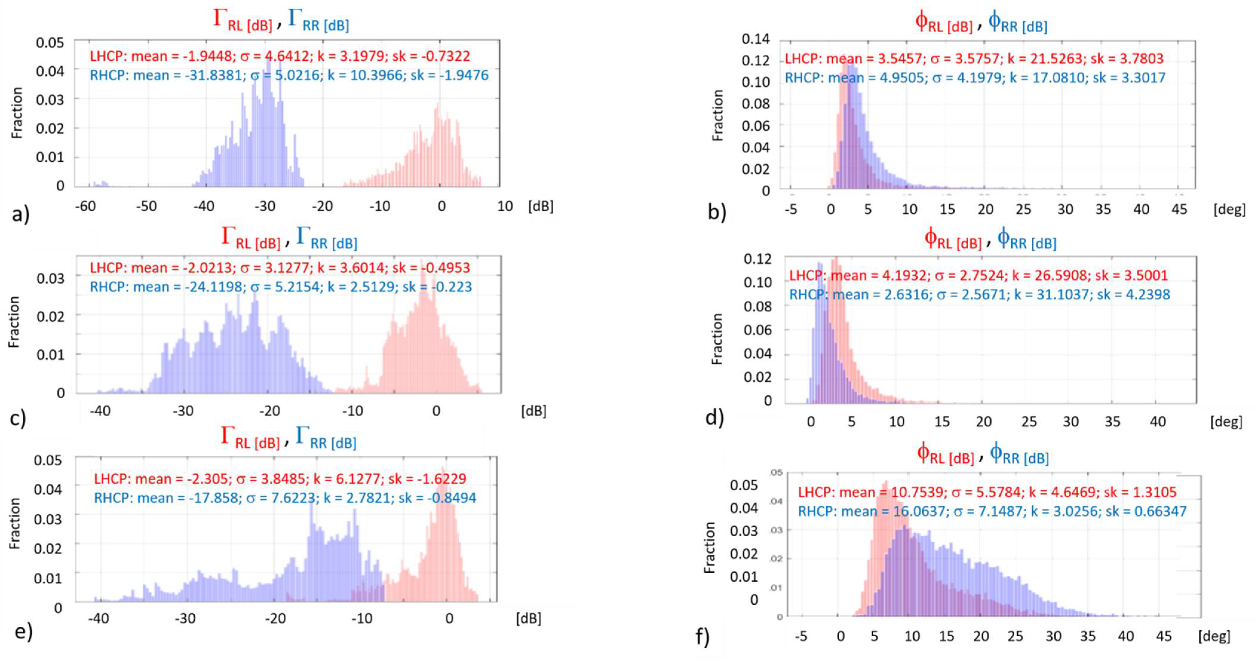
Figure 10 shows the PDFs of the reflection coefficients amplitude [dB] and phase [deg] for clean roughed water surface (significant wave height = 9 cm) without capillary waves and elevation angles of 30°, 45°, and 60°.

In the amplitude (Figure 10a,c,e), the effect of the elevation angle is the opposite at RL and RR polarizations: while at RL polarization the kurtosis (k) and the skewness (sk) increase, most notably from 45° to 60° elevation angles (k from 3.2–3.6 to 6.1, and sk from −0.5–−0.7 to −1.6), indicating a transition from a Gaussian behavior to a more Ricean one, i.e., with a stronger coherent component, at RR polarization it is the opposite, but it occurs mostly from 30° to 45° (k from 10.4 to 2.5–2.8, and sk from −1.9 to −0.2–−0.8), showing a decrease of the coherent component and an increase of the incoherent one.

In the phase (Figure 10d,f), the behavior is more similar at both RL and RR polarizations, showing a transition between 45° to 60° elevation angles, when the mean and standard deviation significantly increase, and the kurtosis and skewness rapidly drop (e.g., k drops from 26.6 and 31.2 at 45° elevation angle to 4.6 and 3.0 at 60° elevation angle).

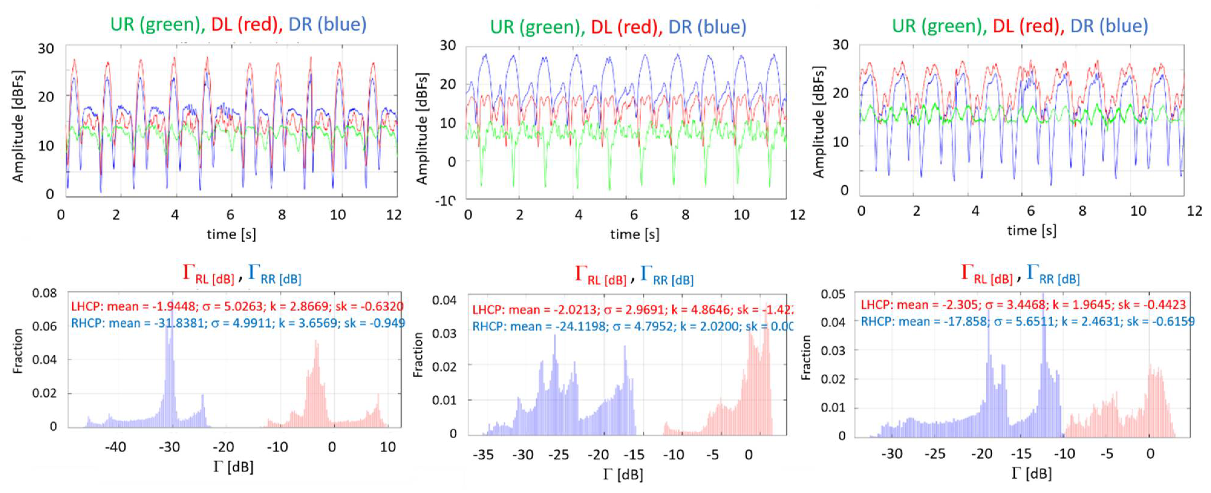
Finally, Figure 11 shows the time series and PDFs of the amplitude of the reflection coefficients [dB] as in Figure 11, but for a clean sinusoidal water surface (significant wave height = 9 cm) without capillary waves, and elevation angles of 30°, 45°, and 60°. Although during the planning of the field experiment using these as reference profiles was considered, the observed quasi-periodic behavior is obviously too artificial, and clearly not representative of the natural conditions. In all the subsequent tests with floating debris, the JONSWAP spectrum was used.

3.2. Marine Plastic Debris

Figure 12 shows the temporal series of the amplitude of the reflected signals [dBfs], and the histograms of the calibrated reflectivity at RL and RR polarizations for the different marine plastic debris tested, at 30° elevation angle. As it will be shown the detectability of marine plastic litter based on amplitude measurements is challenging, even when plastic debris are occupying a significant fraction of the first Fresnel zone (Table 2). This is due to the small dielectric constant change with respect that of water), and the small surface roughness change induced by the floating debris. However, in some cases, the presence of debris may flatten the surface, as in the case of nets or plastic bags (Figure 12a, red ellipse), while in others small capillary waves are induced when a wave crest impinges in the debris (Figure 12b–g, blue ellipses). This is discussed in more detail in Section 4. These small changes are very difficult to detect in terms of the average received power, but induce some detectable changes in the standard deviation of the reflected signal power (i.e., reflectivity), its kurtosis, and/or skewness.

In general, when the kurtosis increases in the amplitude histograms, the skewness decreases, and vice-versa, and in the phase histograms, both tend to either increase or decrease simultaneously. Most detectable changes occur at RL polarization, but often the signature in the RR polarization is evident as well, as cross-polarization is very sensitive to surface roughness.

4. Discussion

Table 4. Summary table of amplitude and statistical descriptors of different experiments: color code indicates the range of variability with respect to the reference scenario (same surface state and geometry conditions, without litter, in the same Table): <−2 u, [−2,−1), [−1,−0.5), [−0.5, +0.5), [+0.5,+1], (+1,+2], >+2 u, where u = units (dB or degrees).

summarizes the main descriptors of all scenarios, and includes a brief description of their main parameters. Numerical results (dB or degrees) are color-coded according to their detectability (gray: not detectable, blue/red: detectable negative/positive changes). As it can be appreciated, while for clean water there are detectable changes in the mean received power as a function of the elevation angle, and most notable a RR polarization, all changes in the average reflection coefficient with respect to their corresponding clean water references (same conditions) are undetectable; there are only small changes in the phase. However, this situation is not encountered in spaceborne GNSS-R receivers, as they have to perform long incoherent averages, and phase information is lost. In addition to the difficulties to detect the small changes in magnitude, absolute calibration errors of GNSS-Reflectometers may prevent the correct interpretation of the results.

Under the presence of litter, in most cases, the RL reflectivity fluctuations increase (e.g., bottles, nets and both, pellets, Styrofoam, caps and lids…), but in some other cases it decreases or it decreases for some elevation angles and/or rms surface height (e.g., JONSWAP SWH = 9 cm, and elevation angle = 45°). At RR polarization, the standard deviation, kurtosis and skewness tend to decrease. The behavior for the phase follows that of the reflectivity fluctuations. The kurtosis behavior is very erratic (either it increases or decreases), but changes are significant. For bottles and fixed net, food wraps and bags, straws, and pellets, the phase of the reflection coefficients is linearly correlated.

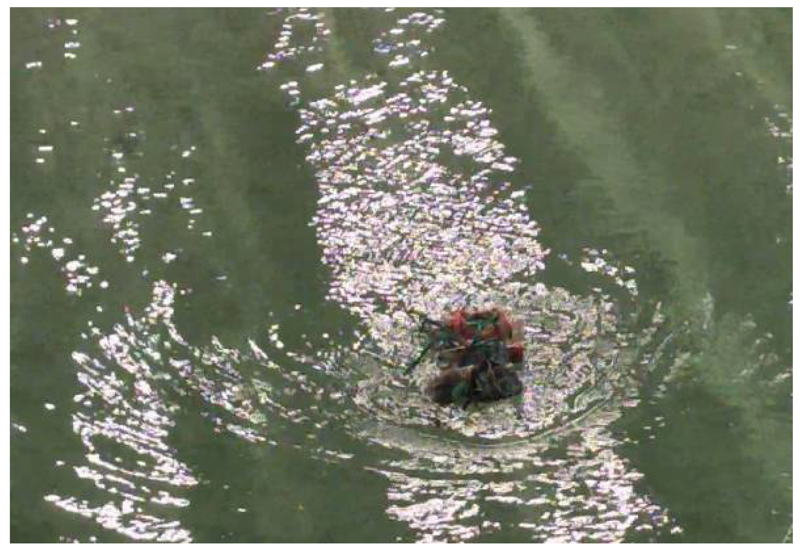
In Section 3 it was discussed that debris pieces are difficult to observe, and even with the sensitivity of our system, and holding the debris in the middle of the Fresnel zone in a flat water surface, they were not directly detectable. However, when the water is roughened, they may either flatten the surface (Figure 12, red ellipses), as in the case of nets or plastic bags, while in others they can create small waves, thus increasing the short waves roughness (Figure 12, blue ellipses). This is illustrated in Figure 13: when a long wave crest (almost vertical long glittering strip) reaches an ensemble of debris (in this case bottles and plastic net) scattered waves are originated are depart from them describing concentric wavefronts, as illustrated in Figure 13, translating into small fluctuations in the received signal power (zooms in Figure 12).

Table 5. Summary table of sensitivities of most “promising observables” to detect marine plastic litter. Color indicates: green = possible, orange = difficult, red = very difficult, and black = marginal.

summarizes the sensitivities of the reflectivity amplitude and phase for all scenarios. The most promising observable is the fluctuation (standard deviation) of the reflectivity, which decreases sharply when there are waves, and increases a bit when capillary waves are present. Not surprisingly, apart from the changes when the water surface becomes rough (first row), the types of marine litter than offer the highest chances to be detected are bottles and fixed net, food wraps and bags, and nets, as they are the ones that dampen the most the water surface (long waves) despite some of them also induce smaller concentric waves when a wave crest impinges over them (Figure 13).

The detectable changes that can be distinguished as follows: (1) in some cases in the std, although it requires a very good absolute calibration, or (2) in the kurtosis of the amplitude and/or the phase, and (3) in some occasions, in the skewness as well. In this sense, the proposed observables: the kurtosis and the skewness of the amplitude PDF (and the phase PDF as well, if feasible at all) can provide an alternative, robust means to detect these anomalies in the received signal, and potentially detect marine plastic litter.

Using the Cox and Munk (1954) [17] model, the effect of surface roughness and the presence of oil on the surface was incorporated in the Zavorotny-Voronovich equation. The peak of the Delay Doppler Map (DDM) was then computed as a function of elevation angle, and wind speed. Results presented in [18] show the DDM peak change due to wind speed for clean water, and its increase due to the presence of oil, with respect to the DDM computed for the same 10-m height wind speed (U₁₀), sea surface salinity (SSS), and sea surface temperature (SST) in clean water. It is worth noting the very significant increase of the DDM peak due to the damping of the capillary waves by oil spills, which produce a stronger forward scattering.

5. Conclusions

This manuscript has described the field experiment conducted by UPC at the Deltares (Delft, The Netherlands) “Atlantic Basin”, as part of the GLIMPS project led by DEIMOS UK for ESA, to study the potential of GNSS-Reflectometry for marine plastic litter detection from space. The experimental set-up, data acquired, the data processing, and the main difficulties encountered have been presented.

A novel approach to process GNSS-R observables has been presented. It is based on the change of some statistical descriptors of the amplitude and phase histograms of the measured instantaneous reflectivity. These observables are:

• The standard deviation of the estimated reflectivity (or received signal power, or DDM peak), which decreases sharply when passing from flat to rough surface, increases a bit when there are capillary waves, and in general increases when there is marine litter;
• The standard deviation of the phase (phase of peak of DDM, computed at 1 ms coherent integration time, and without any incoherent averaging) can also be used;
• The kurtosis and skewness can also be used, as they vary very significantly. In the RL amplitude histogram the kurtosis and the skewness increase, while at RR the kurtosis decreases, and the skewness increases.

The use of the first one requires an accurate absolute calibration, which may be difficult to achieve in real GNSS-R instruments. The second one is also impractical in spaceborne instruments, as significant incoherent averaging is required to increase the carrier-to-noise ratio. The kurtosis and skewness variations offer, in principle, the capability to detect anomalous reflectivity behavior with respect to the reference cases (same marine litter, same wave and observation conditions).

Under the experimental conditions presented, the types of marine litter that can possibly be detected are bottles and fixed nets, food wraps and bags, and nets, as they are the ones that dampen the most the long waves of the water surface.

The extrapolation of these results to the airborne and spaceborne cases is not straightforward and it has to be done with care, as the results presented here have been obtained for 1 ms coherent integration time, without incoherent averaging, and do not include the following effects:

• The different surface roughness in the gyres, regardless of the presence–or not–of marine litter;
• The presence of biofouling and associated increased wave damping;
• The spatial averaging linked to the higher platform height. In the airborne case as the first Fresnel zone from a 1 km height GNSS-R receiver is ~10 m, which is of the order of magnitude of the averaging time (seconds to tens of seconds) times the speed of propagation of the waves in the flume. However, in the spaceborne case, because from LEO the First Fresnel zone is ~300–500 m (depending on the incidence angle), the averaging should be conducted over much longer periods of time.

Despite the fact that there is evidence that the coherent component exists, and that it can be related to long waves, such as swell, etc. [19], as the receiver’s height increases, the coherent scattering component decreases and the incoherent one increases (Table 1 of [20]). In the incoherent case, the received power is the sum of the different power contributions from the fields scattered from different individual surface patches. Therefore, the temporal averaging of our experimental results can be reasonably extrapolated to other configurations, as long as the averaging time is long enough to include many long waves (i.e., mean values in Table 4). Detectability will have to be assessed separately, after an appropriate compensation for the fraction of the surface occupied by damped waves, and the signal-to-noise ratio including geometry, integration time, and receiver parameters, notably antenna directivity.