Visible Near-Infrared Spectroscopy and Pedotransfer Function Well Predict Soil Sorption Coefficient of Glyphosate

Abstract

The soil sorption coefficient (K_d) of glyphosate mainly controls its transport and fate in the environment. Laboratory-based analysis of K_d is laborious and expensive. This study aimed to test the feasibility of visible near-infrared spectroscopy (vis–NIRS) as an alternative method for glyphosate K_d estimation at a country scale and compare its accuracy against pedotransfer function (PTF). A total of 439 soils with a wide range of K_d values (37–2409 L kg⁻¹) were collected from Denmark (DK) and southwest Greenland (GR). Two modeling scenarios were considered to predict K_d: a combined model developed on DK and GR samples and individual models developed on either DK or GR samples. Partial least squares regression (PLSR) and artificial neural network (ANN) techniques were applied to develop vis–NIRS models. Results from the best technique were validated using a prediction set and compared with PTF for each scenario. The PTFs were built with soil texture, OC, pH, Fe_ox, and P_ox. The ratio of performance to interquartile distance (RPIQ) was 1.88, 1.70, and 1.50 for the combined (ANN), DK (ANN), and GR (PLSR) validation models, respectively. vis–NIRS obtained higher predictive ability for K_d than PTFs for the combined dataset, whereas PTF resulted in slightly better estimations of K_d on the DK and GR samples. However, the differences in prediction accuracy between vis–NIRS and PTF were statistically insignificant. Considering the multiple advantages of vis–NIRS, e.g., being rapid and non-destructive, it can provide a faster and easier alternative to PTF for estimating glyphosate K_d.

1. Introduction

Glyphosate [N-(phosphomethyl) glycine] is a post-emergent and non-selective herbicide used worldwide for weed control [1,2,3,4,5]. After application, it sorbs strongly to soil compared to other pesticides such as 2,4-D, Lindane, and paraquat [6]. However, there is still a risk that it can leach with soil colloids [7,8]. Hence, glyphosate can be found in ground and surface water [4,9], presenting a potential threat to aquatic ecosystems [5]. The transfer and dispersion of a pesticide from terrestrial to aquatic ecosystems are largely controlled by its sorption to soil [9,10]. Therefore, the soil sorption coefficient (K_d) is an important input parameter in pesticide fate modeling [11,12]. The K_d of a pesticide depends on the physical and chemical properties of soil and pesticide [13,14]. Hence, a good understanding of the pesticide sorption mechanism and consideration of associated soil properties involved in sorption is required to accurately predict the pesticide retention in soil [15].

Containing three polar functional groups (amine, carboxylate, and phosphate), glyphosate shows a unique binding mechanism with different components in soil [9,10]. It sorbs strongly to the soil mineral fractions, having a high affinity for aluminum and iron oxides [9,10,16,17]. In addition, glyphosate can also be adsorbed to the soil organic matter (SOM) by forming hydrogen bonds with humic substances [18]. However, several studies reported that SOM could be a competitor of glyphosate for adsorption sites [19,20]. Apart from SOM, phosphorous also competes with glyphosate for sorption sites, as the sorption mechanism for those two elements on clay minerals and amorphous oxides are the same [10,21,22]. Other soil properties, such as pH and electrical conductivity (EC), may also influence glyphosate sorption [16,17,22,23,24]. Hence, the risk of glyphosate leaching may differ because of the spatial variation of soil properties.

The glyphosate K_d can be estimated using direct laboratory measurement techniques such as the batch equilibrium test, soil column measurements, etc. [14]. However, those methods are cost- and time-intensive and not suitable when the glyphosate K_d needs to be measured on large spatial scales or at high spatial sample resolution. In this connection, a few studies estimated the glyphosate K_d with a limited number of easily measurable soil properties. As an example, Paradelo et al. [24] developed PTFs to predict the glyphosate K_d for two loamy agricultural fields in DK as a function of the best four contributing parameters (e.g., a combination of clay, Fe_ox, Olsen P, and pH; or clay, OC, Olsen P, and EC). In contrast to Paradelo’s field-scale study, Dollinger et al. [16] assembled a database of soil properties (data obtained from 23 studies on soils and sediments of four different continents: Europe, Asia, North, and South America) and established a PTF to predict the glyphosate K_d by incorporating only two parameters: clay and cation exchange capacity (CEC).

Visible near-infrared diffuse reflectance spectroscopy (vis–NIRS: 400–2500 nm) is an alternative to conventional soil testing techniques [25,26,27,28]. Soil properties such as clay minerals, SOM, and iron and aluminum oxides have direct spectral responses in this electromagnetic range [29]. Since those soil properties have been found to be some of the main controllers of glyphosate sorption, successful estimation of the glyphosate K_d using laboratory vis–NIRS has been shown [30]. Soil properties show a large variation across sites, making laboratory vis–NIRS prediction less accurate, specifically for large spatial-scale studies compared to field-scale studies [31]. Thus, vis–NIRS analysis requires sophisticated statistical techniques to correlate soil spectra with soil properties of interest. Partial least squares regression (PLSR) is a popular linear multivariate data analysis (MVDA) technique for soil quantitative analysis from the perspective of being rapid and easy to derive and interpret the outcomes [27]. However, the PLSR method has shortcomings in prediction accuracy when the soil properties are not linearly correlated with spectral intensities. Artificial neural network (ANN) is a machine learning technique that potentially can tackle better non-linearity issues than the PLSR [32,33].

In comparison to a vast number of studies dedicated to the use of vis–NIRS for the key soil properties’ estimation, so far, only two studies documenting the potential of vis–NIRS to predict the K_d of the glyphosate have been published. These studies represent rather small-scale investigations (field and regional) based on small numbers of samples and with the use of only linear MVDA. Paradelo et al. [30] conducted a field-scale investigation in a Danish agricultural field by incorporating vis–NIRS with the PLSR technique. The authors reported successful estimations of K_d values but emphasized a need for more research, including diverse soil types representing different geographical scales and samples from both national and field investigations. Moreover, since only 45 samples were used in their study, only a leave-one-out cross-validation model was developed, and no validation of model performance was provided using a separate prediction set. Later, Hermansen et al. [34] reported on a regional-scale study including 26 sites on New Zealand’s South Island. Successful estimates of glyphosate K_d were obtained, yet as in the case of the previous study, due to the limited sample number, only cross-validation was possible. Thus, the results of the above-mentioned studies do not provide estimates of the robustness of the developed models. To the best of the author’s knowledge, no studies of vis–NIRS measurements have yet been reported to predict the glyphosate K_d on soil samples originating from two countries and covering a wide range of K_d values. Moreover, no studies were found to document the effect of applying models dedicated to one geographic origin/country in comparison to applying a model combining both on the final predictive ability for glyphosate K_d. Moreover, the potential of non-linear modeling techniques to predict glyphosate K_d has not been investigated yet.

Remote sensing (RS), including multispectral and hyperspectral imagery, is tested for soil properties estimation on large spatial scales [35,36,37]. In general, poorer relationships between soil properties and spectral features of satellite imaging spectroscopy as compared to the relationships between soil properties and laboratory spectroscopy are achieved due to, for example, the weather conditions, land cover, the spectral resolution of the sensors, etc. [38]. A few studies reported a successful application of image processing technology to overcome the limitation of using low-resolution images for land-cover mapping [39,40]. Thus, there is a potential for hyperspectral (e.g., HYPERION), multispectral (e.g., LANDSAT-8), and super spectral (e.g., SENTINEL-2) satellite optical data for estimating and monitoring of the glyphosate K_d. However, it is crucial to gain a better understanding of the capabilities of laboratory spectroscopy for the estimation of glyphosate K_d on a larger scale and to address the above-mentioned knowledge gaps before testing the RS techniques.

The aim of this study was to test the feasibility of vis–NIRS to estimate the glyphosate K_d for a wide range of soil types collected from Denmark (DK) and Greenland (GR) in comparison with PTF. To serve the purpose of the study, predictive models were generated considering two scenarios: (i) one general model based on the DK and GR soil samples together and (ii) individual models based on the DK and GR soils separately. Both linear (PLSR) and non-linear (ANN) techniques were applied to develop vis–NIRS models. A comparison of the accuracy between those two spectral modeling techniques was carried out, and the spectral model that resulted in the lowest prediction error was compared with PTF for each scenario. Finally, a validation of the models was conducted using a subset of samples not included in the calibration step.

2. Materials and Methods

2.1. Soil Samples

A total of 439 cultivated soil samples from DK (n = 296) and GR (n = 143) representing different spatial scales (field sampling from 15 DK and GR fields and point sampling across DK) were collected for this study (Figure 1). A wide variety of fields were included to cover different agricultural soil types from DK. Soils from the DK fields were sampled from a depth of 0–25 cm and in a grid of 15 by 15 m. Additionally, single-point sampling was conducted from a depth of 0–25 cm across DK. The GR soils were sampled from the A horizon of 0–15 cm depth and in rectangular grids with either 7.5 m or 15 m spacing. Two of the GR fields were adjacent and, thus, represented by one location (marked with a red circle in Figure 1b).

The two countries represent soils of different parent materials and the degree of their variation. The parent material of DK samples is more variable than that of GR samples. It consists of soils developed on Weichsel glacial deposits, mainly tills, Saale glacial deposits, and the younger Weichsel outwash plain, marine, sand dune, and salt marsh deposits [41]. According to Moberg [42], illite is the dominant clay mineral for the DK soils. The soil texture mainly ranges from sandy to silty clay loam. More information about the DK soil types can be found in Breuning–Madsen and Jensen [41]. The geology of southwest GR presents a much more uniform characteristic. The GR fields can be separated into glaciofluvial deposits and aeolian deposits, where all soils are developed on granodioritic gneiss and granites, and the soil texture mainly ranges from loamy sand to silty loam [43,44]. Since the two countries represent differences in geologies and, thus, differences in soils, two separate datasets were developed and defined as follows. (i) A DK dataset, including samples from DK, and (ii) a GR dataset, including samples from GR. Apart from these two datasets, a combined dataset was also developed, which included samples from both DK and GR.

2.2. Laboratory Analysis

The soil samples were air-dried, crushed, and passed through a 2-mm sieve. Particle size distribution was determined by a combination of wet sieving, pipette, and hydrometer methods, as described by Gee and Or [45]. To determine the TOC on ball-milled samples, an organic elemental analyzer was coupled with a thermal conductivity detector (Thermo Fisher Scientific, Waltham, MA, USA) and oxidized the samples at 950 °C. As K_d is dependent on both soil mineral and organic fractions, the texture and organic matter were standardized to 100%. The soil pH was measured in water by following the procedure described by Thomas [46]. The EC was measured in a soil/water extract of 1:9 by volume. Oxalate extractable aluminum (Al_ox), iron (Fe_ox), and phosphorous (P_ox) were measured using the method of Schoumans et al. [47]. The glyphosate K_d was measured with a batch equilibration test following Soares et al. [48]. The measurements of glyphosate K_d for two DK fields can be found in Paradelo et al. [24]. The remaining glyphosate K_d measurements were not published previously.

2.3. Visible Near-Infrared Measurements and Analysis

The vis–NIRS measurements were performed on air-dried and 2-mm sieved samples with a vis–NIR spectrometer (DS2500, Foss) covering a spectral range of 400–2500 nm with 0.5 nm resolution. A quartz sample cup with a diameter of 7 cm was used for measurement. The cup was rotated inside the spectrometer and the bottom of the cup was scanned at seven different positions to collect the reflectance (R). The scanning was performed four times at each position. The 28 spectra for each soil sample were subsequently averaged into one representative soil spectrum. The absorbance (A) spectrum for each sample was calculated by A = [log(R⁻¹)].

2.4. Data Subdivision and Exploratory Analysis

A simple graphical representation of the data analysis process for predicting the K_d of glyphosate is presented in Figure 2. The investigated dataset comprises both field and point samples collected from two countries. As described above, soils collected from Denmark represent soils developed on different parent materials, whereas Greenlandic samples present soils of a more uniform geology. The samples within each of the included fields are naturally of the same parent material; however, in order to avoid the issue of pseudoreplicates, they were selected to cover a wide range of soil texture or soil organic carbon and, consequently, represent wide gradients in K_d values. As parent material affects the composition of the soil matrix, its effect is further manifested in spectral response. To enable a selection of representative calibration samples covering this wide range of parent materials, each dataset was sub-divided into calibration (80% of the total samples) and validation subsets (remaining 20% of the total samples, samples not included, nor influencing the calibration procedure) using the Kennard–Stone sample selection method [49] on the soil spectral data prior to the development of models. Exploratory data analysis was conducted on reference data for outlier detection and to understand the data structure, correlation among soil properties, and the potential of each soil property to explain the variability of K_d (by single linear regression analysis). Exploratory analysis of spectral data, e.g., visual investigation of soil spectra for spectral outlier detection, and principal component analysis (PCA) to identify sample groupings and the relationships among samples and variables, was also carried out [50].

2.5. Pedotransfer Function (PTF)

The simple PTF proposed by Dollinger et al. [16] could not be applied here due to the unavailability of the CEC measurements for all samples. Hence, a PTF based on available data in the current study was developed. Forward multiple linear regression (MLR) analysis was conducted to find a subset of soil properties that best explained the variation of K_d. Then, the PTFs were built using those soil properties (i.e., texture, OC, pH, Fe_ox, etc.). However, a general PTF was generated with all soil samples prior to developing the PTFs on the combined DK and GR calibration subsets. The purpose of generating a general PTF was to compare the MLR models’ accuracy developed on the combined dataset and the combined calibration subset.

2.6. Spectral Modeling

The Matlab program PLS Toolbox version 8.6.2 (Eigenvector Research Inc., Wenatchee, WA, USA) was used to develop the vis–NIRS models using the combined, DK, and GR calibration subsets separately. Spectral pretreatment techniques such as scatter corrections (e.g., multiplicative scatter corrections—MSC and standard normal variate—SNV) and spectral derivatives (e.g., Savitzky–Golay—SG polynomial derivative filters) were applied to resolve the overlapping bands and to decrease the scatter and baseline effects [51]. A few possible combinations of those techniques were also tested. The PLSR and ANN techniques were used consecutively on both raw and pre-processed spectra for developing spectral models on each calibration subset.

Partial least squares regression uses data compression techniques and compresses the highly collinear predictor variables to a few orthogonal factors, designated as latent variables (LVs) [52]. Those LVs were further used to develop a predictive linear model by maximizing the covariance between spectral data and reference data of soil properties. The optimal number of LVs in the PLSR calibration models was defined as the number of LVs after which RMSE no longer decreased meaningfully [53]. In this study, the PLSR regression coefficients (RC) were investigated to identify the important wavelength for predicting glyphosate K_d.

Artificial Neural Network is a machine-learning algorithm designed to simulate how a human brain analyzes and processes information [54]. An ANN comprises three layers of interconnected nodes: the input layer (here, vis–NIR spectra), the hidden layer, and the output layer (soil properties to be predicted). The nodes are called artificial neurons, and the connections between two nodes are termed edges. Neurons and edges usually have a weight that is adjusted by the network itself with the training process [32]. The vis–NIR spectra were compressed with the PLSR to shorten the computation time for the current study. Then, the ANN analysis was performed with the two nodes in the first layer. The number of variables for each ANN model was equal to the number of LVs of the respective PLSR model.

2.7. Models’ Validation

The most optimal spectral and PTF calibration models were validated using the prediction set for each dataset. Further, validation results from the individual DK and GR models were joined and models’ statistics (RMSE_P and R²) were recalculated to compare with the results of the combined validation model. This was performed for both the PTFs and vis–NIRS models. The purpose was to enable a fair comparison of validation results using the same range of K_d values in the validation dataset and understand whether developing country-based models is more beneficial than using a combined calibration model.

To evaluate the models’ performance, the ratio of performance to interquartile distance (RPIQ) values were also used along with R² and RMSE. The RPIQ is generally used to standardize the value of standard error with respect to the natural dispersion of the samples [25]. Thus, the RPIQ value is useful for model performance evaluation when the comparison of model performance is carried out among different datasets for the same soil properties.

RPIQ = (Q3 − Q1)/RMSE

(1)

Here, Q3 − Q1 is the interquartile range (IQR) and RMSE is the root mean square error which can be calculated from the following equation.

$$RMSE=\sqrt{\frac{{\sum }_{i=1}^N{\left(Actua{l}_i-Predicte{d}_i\right)}^2}{N}}$$

(2)

Here, Actual_i and Predicted_i are the reference and predicted values of glyphosate K_d, respectively, for the same sampling unit, and N is the total number of samples.

3. Results

3.1. Exploratory Analysis

3.1.1. Soil Properties

Descriptive statistics of soil properties for the combined, DK, and GR datasets are summarized in

Table 1. Descriptive statistics of soil properties for all datasets, including their respective calibration and validation subsets.

Statistical Parameters	Clay	Silt	Sand	TOC a	Kd b	pH	EC c	Feox d	Alox d	Pox d
	%				L kg−1	(-)	mS cm−1	mmol kg−1
Combined dataset, n = 439 (Calibration, n = 351) (Validation, n = 88)
Mean	11 e (11 f) (11 g)	11 (11) (12)	73 (74) (73)	2.6 (2.7) (2.0)	448 (452) (431)	6.3 (6.3) (6.4)	0.6 (0.7) (0.5)	54.4 (56.2) (47.2)	37.0 (38.5) (31.1)	15.9 (16.6) (13.1)
Max	69 (69) (40)	43 (43) (42)	94 (94) (93)	8.4 (8.4) (7.6)	2409 (2409) (2149)	8.3 (8.3) (7.7)	3.9 (3.9) (2.1)	300.0 (300.0) (190.0)	130.0 (130.0) (110.0)	52.0 (52.0) (41.0)
Min	2 (2) (2)	2 (2) (2)	11 (11) (13)	0.8 (0.8) (1.1)	37 (37) (93)	4.4 (4.4) (4.8)	0.1 (0.1) (0.2)	8.3 (8.3) (9.9)	11.0 (11.0) (16.0)	1.5 (1.5) (7.1)
Median	10 (9) (13)	11 (11) (14)	74 (75) (70)	2.1 (2.2) (1.9)	378 (369) (423)	6.4 (6.3) (6.6)	0.5 (0.6) (0.5)	44.0 (45.0) (44.0)	33.0 (35.0) (29.0)	12.0 (13.0) (11.0)
CV h	0.8 (0.9) (0.5)	0.6 (0.6) (0.5)	0.2 (0.2) (0.2)	0.5 (0.5) (0.4)	0.7 (0.8) (0.6)	0.1 (0.1) (0.1)	0.6 (0.6) (0.5)	0.8 (0.8) (0.5)	0.4 (0.4) (0.4)	0.5 (0.5) (0.5)
Q1 i	4 (4) (6)	6 (6) (5)	66 (66) (65)	1.6 (1.7) (1.6)	242 (238) (277)	5.7 (5.7) (5.9)	0.4 (0.4) (0.4)	33.0 (32.0) (36.0)	26.0 (26.0) (25.0)	9.9 (10.0) (9.5)
Q3 j	15 (15) (15)	16 (15) (16)	84 (84) (83)	3.0 (3.3) (2.1)	519 (546) (494)	6.8 (6.8) (6.8)	0.8 (0.8) (0.6)	60.0 (62.2) (50.0)	46.0 (48.0) (36.0)	20.0 (21.0) (13.0)
Denmark, n = 296 (Calibration, n = 228) (Validation, n = 68)
Mean	14 e (15 f) (14 g)	13 (13) (15)	68 (69) (68)	2.2 (2.3) (2.0)	410 (406) (424)	6.6 (6.6) (6.6)	0.7 (0.7) (0.6)	47.4 (48.0) (45.3)	31.7 (32.5) (28.7)	13.1 (13.5) (12.0)
Max	69 (69) (40)	43 (43) (42)	91 (91) (90)	8.4 (8.4) (7.6)	2409 (2409) (2149)	8.3 (8.3) (7.7)	3.9 (3.9) (2.1)	240.0 (240.0) (190.0)	130.0 (130.0) (110.0)	32.0 (32.0) (28.0)
Min	3 (3) (3)	3 (3) (3)	11 (11) (13)	0.8 (0.8) (1.1)	37 (37) (93)	4.9 (4.9) (5.5)	0.2 (0.2) (0.3)	8.3 (8.3) (9.9)	11.0 (11.0) (16.0)	3.9 (3.9) (7.1)
Median	13 (13) (14)	14 (13) (16)	69 (70) (66)	1.9 (1.9) (0.2)	345 (310) (408)	6.7 (6.6) (6.7)	0.5 (0.6) (0.5)	40.0 (39.0) (43.0)	28.0 (28.0) (28.0)	11.0 (11.0) (11.0)
CV h	0.6 (0.7) (0.3)	0.5 (0.5) (0.3)	0.2 (0.2) (0.1)	0.5 (0.5) (0.4)	0.8 (0.9) (0.7)	0.1 (0.1) (0.1)	0.6 (0.6) (0.5)	0.8 (0.9) (0.6)	0.5 (0.5) (0.4)	0.4 (0.4) (0.4)
Q1 i	10 (9) (12)	10 (9) (13)	64 (64) (65)	1.6 (1.6) (1.6)	208 (197) (272)	6.3 (6.2) (6.4)	0.4 (0.5) (0.4)	29.0 (28.0) (34.8)	23.1 (23.7) (22.8)	9.6 (9.8) (9.4)
Q3 j	16 (17) (15)	16 (16) (17)	76 (77) (72)	2.3 (2.4) (2.1)	485 (493) (477)	6.9 (7.0) (6.8)	0.8 (0.9) (0.6)	48.0 (49.0) (47.3)	35.3 (37.3) (30.0)	15.0 (16.0) (13.0)
Greenland, n = 143 (Calibration, n = 123) (Validation, n = 20)
Mean	4 e (4 f) (3 g)	7 (8) (4)	84 (83) (90)	3.2 (3.4) (2.1)	526 (537) (455)	5.6 (5.6) (5.5)	0.5 (0.5) (0.3)	68.9 (71.4) (53.9)	48.1 (49.5) (39.4)	21.5 (22.3) (16.6)
Max	9 (9) (4)	30 (30) (9)	94 (94) (93)	7.8 (7.8) (4.7)	1414 (1414) (757)	7.4 (7.4) (6.0)	1.4 (1.4) (0.7)	300.0 (300.0) (82.0)	97.0 (97.0) (53.0)	52.0 (52.0) (41.0)
Min	2 (2) (2)	2 (2) (2)	58 (58) (80)	0.9 (0.9) (1.2)	57 (57) (197)	4.4 (4.4) (4.8)	0.1 (0.1) (0.2)	22.0 (22.0) (22.0)	18.0 (18.0) (30.0)	1.5 (1.5) (8.2)
Median	3 (4) (3)	6 (7) (3)	84 (83) (91)	3.0 (3.1) (1.8)	472 (472) (469)	5.5 (5.5) (5.4)	0.4 (0.5) (0.2)	57.0 (60) (55.0)	46.0 (46.0) (38.0)	21.0 (22.0) (14.5)
CV h	0.3 (0.3) (0.2)	0.7 (0.6) (0.5)	0.1 (0.1) (0.0)	0.4 (0.4) (0.5)	0.5 (0.6) (0.4)	0.1 (0.1) (0.1)	0.6 (0.6) (0.5)	0.7 (0.7) (0.3)	0.3 (0.3) (0.2)	0.5 (0.5) (0.5)
Q1 i	3 (3) (2)	4 (4) (3)	79 (78) (89)	2.1 (2.4) (1.5)	321 (319) (376)	5.2 (5.2) (5.3)	0.3 (0.3) (0.2)	46.5 (46.5) (46.5)	38.0 (39.0) (35.3)	11.0 (12.0) (10.7)
Q3 j	4 (4) (3)	9 (9) (4)	90 (89) (92)	4.1 (4.3) (2.2)	656 (669) (517)	5.9 (5.9) (5.8)	0.7 (0.7) (0.3)	74.0 (77.0) (63.3)	54.0 (57.5) (42.0)	29.0 (30.0) (18.0)

^a TOC, total organic carbon; ^b K_d, soil sorption coefficient of glyphosate; ^c EC, electrical conductivity; ^d Fe_ox, Al_ox, and P_ox, oxalate-extractable iron, aluminum, and phosphorous; ^e statistics of all soil samples for each dataset; ^f statistics for the calibration subsets; ^g statistics for the validation subsets; ^h CV, coefficient of variation; ⁱ Q1, first quartile (25th percentile); ^j Q3, third quartile (75th percentile). The sum of the mineral fractions and organic matter content equals 100%.

. Soil samples of the combined dataset encompassed a wide range of soil properties, specifically in terms of texture (e.g., clay: 2–69%) and K_d (37–2409 L kg⁻¹). The high gradient in soil properties of the combined dataset was expected due to the wide spatial distribution of the samples collected from different locations in DK and GR.

The trend of sample distribution demonstrated the presence of a few extreme samples, especially for the combined and DK datasets. For example, the value of glyphosate K_d for 50% of the samples fell between 242 and 519 L kg⁻¹ for the combined dataset and 208 and 485 L kg⁻¹ for the DK dataset; nonetheless, the range of glyphosate K_d was 37–2409 L kg⁻¹ for both datasets (Table 1). Those few extreme samples might cause a high error in predicting the glyphosate K_d and might influence the model statistics. However, those extreme samples were not removed, as the study’s interest was to fit a calibration model for soil samples with a wide range of K_d values.

3.1.2. Soil Spectra

Visual investigation on vis–NIR spectra for all soil samples showed no spectral outliers and noise in any of the datasets (Figure 3a,b). Moreover, the distinction of the soil spectra, e.g., the distinction between the DK and GR datasets, delineated the variability of soil samples present in each dataset due to their different physicochemical properties and parent materials. For example, a distinct feature around 2208 nm was observed for a few DK soil samples, which was not present in the GR soil samples (Figure 3b). Absorption bands near 2200 nm are referred to as clay minerals such as kaolinite, illite, and smectite [27,28].

The principal component analysis (PCA) revealed that the first two principal components (PC1 and PC2) together explained 95% of the spectral variation among soil samples due to their differences in soil physicochemical properties (Figure 3c,d). Loading of the PC1 (Figure 3e) indicated that information along PC1 may be attributed to OM or clay minerals that are dominant hydrated oxides of iron, such as goethite, manifested in a broad positive absorption peak near 600 nm [28,55]. On the other hand, PC2 explained variability in clay mineralogy with a broad absorption peak near 500 nm (presence of minerals containing hydrated oxides of iron such as ferrihydrite and hematite), sharp absorption peaks near 1400 (overtones caused by O–H stretch in clay octahedral layer), 1900 (overtones caused by molecular H₂O), and at 2200 nm (combination vibration of water bound in the clay interlayer lattice) [56,57]. Nevertheless, score plots revealed that the grouping of samples according to OM or Fe_ox along PC1 and sample groupings according to clay content along PC2 could not be detected. Spectral responses to OM and clay content not only rely on the quantity of OM and clay but also on the quality of OM (i.e., humic or fulvic acids) and clay mineralogy. However, detailed information about clay mineralogy and the quality of OM for each sampling location was not available for this study.

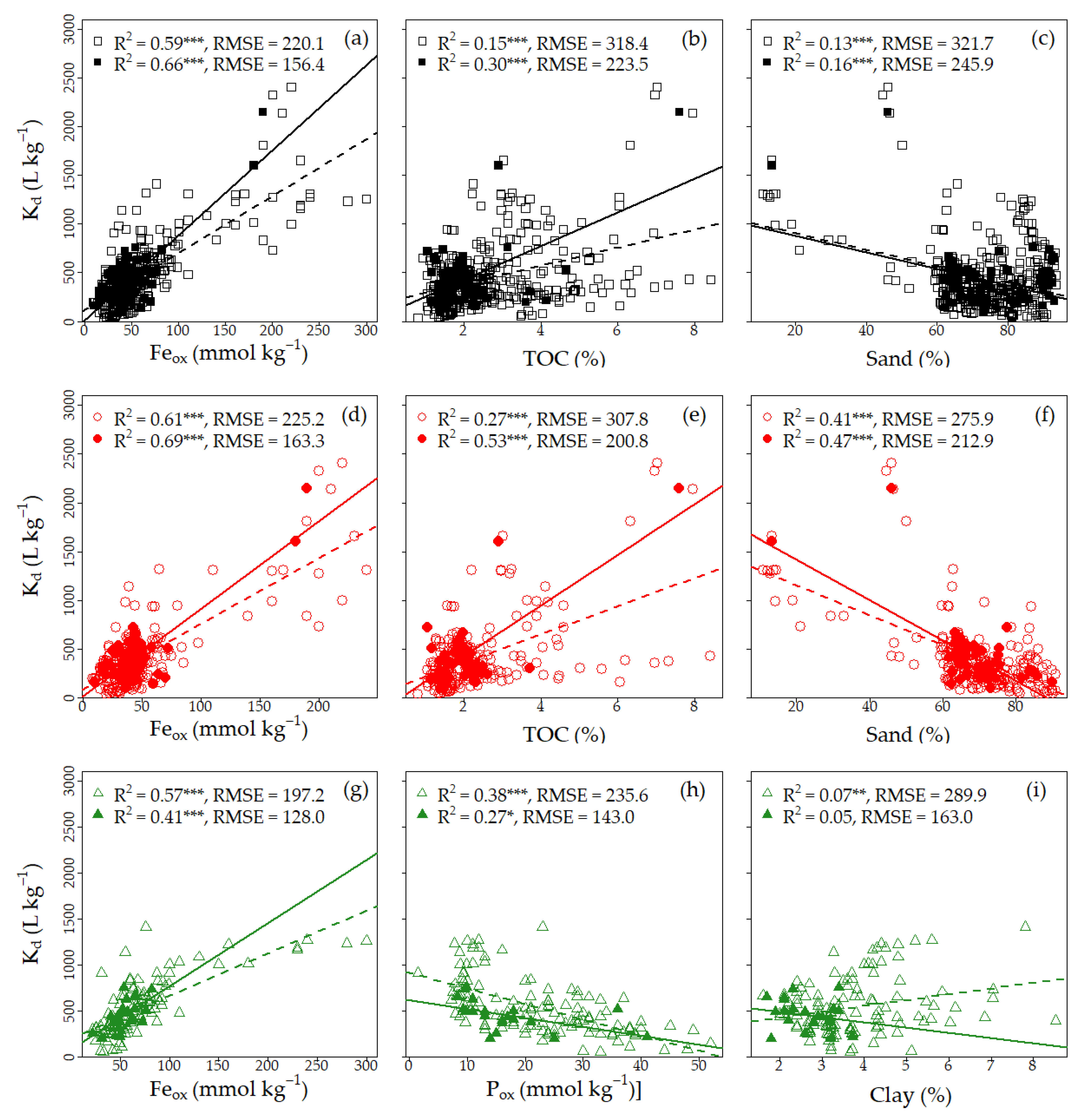
3.1.3. Single Linear Regression (SLR) Analysis

The best three SLR model results of the calibration and validation subsets of each dataset are shown in Figure 4. In general, the trend of correlation was the same for both the calibration and validation subsets of each dataset (

Table A1. Pearson’s correlation matrix of soil physicochemical properties for the combined, Danish, and Greenlandic datasets (including their calibration and validation subsets).

	Clay	Silt	Sand	TOC a	pH	EC b	Feox c	Alox c	Pox c	Kd d
Combined dataset, n = 439 (Calibration, n = 351) (Validation, n = 88)
Clay	1	0.66 ***,e,f (0.62 ***,g) (0.95 ***,h)	−0.92 *** (−0.92 ***) (−0.98 ***)	−0.08 (−0.10) (0.12)	0.58 *** (0.55 ***) (0.76 ***)	0.37 *** (0.36 ***) (0.52 ***)	0.33 *** (0.34 ***) (0.30 **)	−0.29 *** (−0.27 ***) (−0.45 ***)	−0.19 *** (−0.17 **) (−0.34 **)	0.32 *** (0.31 **) (0.37 **)
Silt		1	−0.87 *** (−0.85 ***) (−0.98 ***)	−0.06 (−0.06) (0.10)	0.49 *** (0.45 ***) (0.73 ***)	0.35 *** (0.35 ***) (0.51 ***)	0.16 *** (0.17 **) (0.23 *)	−0.31 *** (−0.28 ***) (−0.43 ***)	−0.17 *** (−0.14 *) (−0.34 **)	0.21 *** (0.20 **) (0.30 **)
Sand			1	−0.09 (−0.08) (−0.23 *)	−0.55 *** (−0.51 ***) (−0.73 ***)	−0.43 *** (−0.42 ***) (−0.55 ***)	−0.34 *** (−0.35 ***) (−0.32 **)	0.24 *** (0.21 ***) (0.43 ***)	0.13 *** (0.10) (0.30 **)	−0.36 ** (−0.36 **) (−0.40 **)
TOC				1	−0.29 *** (−0.31 ***) (−0.13)	0.21 *** (0.17 **) (0.31 **)	0.32 *** (0.30 ***) (0.47 ***)	0.49 *** (0.52 ***) (0.02)	0.41 *** (0.40 ***) (0.30 **)	0.40 *** (0.38 ***) (0.55 ***)
pH					1	0.37 *** (0.38 ***) (0.37 ***)	−0.13 ** (−0.13 *) (−0.05)	−0.43 *** (−0.42 ***) (−0.51 ***)	−0.26 *** (−0.25 ***) (−0.36 ***)	−0.21 *** (−0.23 ***) (−0.06)
EC						1	0.18 *** (0.15 **) (0.36 ***)	−0.06 (−0.07) (−0.24 *)	0.13 ** (0.12 *) (−0.01)	0.02 (0.00) (0.20)
Feox							1	0.18 *** (0.18 ***) (0.09)	0.10 * (0.08) (0.18)	0.77 *** (0.77 ***) (0.81 ***)
Alox								1	0.54 *** (0.51 ***) (0.63 ***)	0.10 * (0.12 *) (−0.03)
Pox									1	−0.15 ** (−0.16 **) (−0.15)
Kd										1
Denmark, n = 296 (Calibration, n = 228) (Validation, n = 68)
Clay	1	0.58 *** (0.56 ***) (0.90 ***)	−0.93 *** (−0.93 ***) (−0.97 ***)	0.15 ** (0.14 *) (0.33 **)	0.40 *** (0.40 ***) (0.48 ***)	0.32 *** (0.32 ***) (0.33 **)	0.74 *** (0.75 ***) (0.67 ***)	−0.07 (−0.05) (−0.33 **)	0.13 * (0.18 **) (−0.33 **)	0.57 *** (0.57 ***) (0.67 ***)
Silt		1	−0.82 *** (−0.81 ***) (−0.96 ***)	0.01 (0.01) (0.16)	0.35 *** (0.33 ***) (0.48 ***)	0.23 *** (0.24 ***) (0.31 **)	0.52 *** (0.53 ***) (0.51 ***)	−0.32 *** (−0.32 ***) (−0.30 *)	−0.28 *** (−0.25 ***) (−0.41 ***)	0.45 *** (0.43 ***) (0.52 ***)
Sand			1	−0.25 *** (−0.24 ***) (−0 37 **)	−0.39 *** (−0.38 ***) (−0.48 ***)	−0.33 *** (−0.34 ***) (−0.37 **)	−0.76 *** (−0.77 ***) (−0.67 ***)	0.13 * (0.10) (0.31 *)	0.03 (−0.02) (0.34 **)	−0.64 *** (−0.64 ***) (−0.69 ***)
TOC				1	−0.15 ** (−0.16 *) (−0.09)	0.14 * (0.11) (0.27 *)	0.34 *** (0.30 ***) (0.61 ***)	0.42 *** (0.49 ***) (−0.11)	0.07 (0.07) (−0.02)	0.54 *** (0.52 ***) (0.73 ***)
pH					1	0.27 *** (0.29 ***) (0.14)	0.10 (0.10) (0.09)	−0.25 *** (−0.22 ***) (−0.41 ***)	−0.01 (0.03) (−0.22)	−0.13 * (−0.15 *) (−0.05)
EC						1	0.36 *** (0.34 ***) (0.52 ***)	−0.02 (−0.02) (−0.15)	0.10 (0.10) (−0.04)	0.12 * (0.10) (0.30 *)
Feox							1	−0.04 (−0.05) (0.02)	0.31 *** (0.32 ***) (0.22)	0.78 *** (0.78 ***) (0.83 ***)
Alox								1	0.45 *** (0.41 ***) (0.65 ***)	−0.03 (−0.03) (−0.06)
Pox									1	−0.05 (−0.04) (−0.11)
Kd										1
Greenland, n = 143 (Calibration, n = 123) (Validation, n = 20)
Clay	1	0.79 *** (0.78 ***) (0.59 **)	−0.85 *** (−0.83 ***) (−0.74 ***)	0.41 *** (0.34 ***) (0.69 ***)	0.11 (0.12) (−0.43)	0.47 *** (0.40 ***) (0.76 ***)	0.28 *** (0.26 **) (0.04)	0.62 *** (0.59 ***) (0.42)	0.31 *** (0.25 **) (0.67 **)	0.26 ** (0.26 **) (−0.21)
Silt		1	−0.93 *** (−0.93 ***) (−0.96 ***)	0.36 *** (0.29 **) (0.88 ***)	0.13 (0.13) (0.03)	0.53 *** (0.48 ***) (0.87 ***)	−0.12 (−0.17) (−0.01)	0.50 *** (0.45 ***) (0.67 **)	0.50 *** (0.46 ***) (0.84 ***)	−0.06 (−0.08) (−0.20)
Sand			1	−0.66 *** (−0.60 ***) (−0.97 ***)	−0.11 (−0.11) (0.14)	−0.68 *** (−0.64 ***) (−0.96 ***)	−0.02 (0.02) (0.07)	−0.57 *** (−0.53 ***) (−0.59 **)	−0.57 *** (−0.53 ***) (−0.86 ***)	−0.01 (0.01) (0.24)
TOC				1	−0.02 (−0.03) (−0.20)	0.70 *** (0.65 ***) (0.96 ***)	0.16 (0.14) (−0.17)	0.38 *** (0.32 ***) (0.47 *)	0.52 *** (0.47 ***) (0.80 ***)	0.03 (0.01) (−0.24)
pH					1	0.43 *** (0.46 ***) (−0.11)	−0.09 (−0.10) (−0.05)	−0.04 (−0.05) (−0.03)	0.11 (0.12) (−0.20)	−0.17 * (−0.19 *) (0.06)
EC						1	0.00 (−0.04) (−0.18)	0.26 ** (0.19 *) (0.50 *)	0.57 *** (0.54 ***) (0.82 ***)	−0.13 (−0.16) (−0.31)
Feox							1	0.30 *** (0.28 **) (0.27)	−0.29 *** (−0.33 ***) (−0.06)	0.75 *** (0.75 ***) (0.64 **)
Alox								1	0.42 *** (0.38 ***) (0.67 **)	0.18 ** (0.17) (0.04)
Pox									1	−0.58 *** (−0.62 ***) (−0.52 *)
Kd										1

^a TOC, total organic carbon; ^b EC, electrical conductivity; ^c Fe_ox, Al_ox, and P_ox, oxalate-extractable iron, aluminum, and phosphorous; ^d K_d, soil sorption coefficient of glyphosate; ^e Pearson correlation coefficient at significance levels of * 0.05, ** 0.01 and *** 0.001; ^f results of all soil samples for each dataset; ^g results for the calibration subsets; ^h results for the validation subsets.

—see Appendix A). Among all soil properties, Fe_ox could explain more than 50% of the sorption variability of glyphosate as a single predictor for all datasets (Figure 4a,d,g). Organic carbon showed a higher positive correlation with the K_d for all datasets except the GR datasets (Figure 4b,e). Soil texture was strongly correlated with K_d for the DK dataset compared to the other two datasets (Table A1). de Jonge et al. [21] found a strong correlation between P_ox and K_d, while P_ox could explain nearly 30% of the variation of K_d of glyphosate only for the GR dataset (Figure 4h). Other soil properties, such as Al_ox [18] and pH [17,22], were also considered important sorbents of glyphosate. However, those two properties showed a weak correlation with the K_d for this study (Table A1).

3.2. Prediction of the K_d of Glyphosate

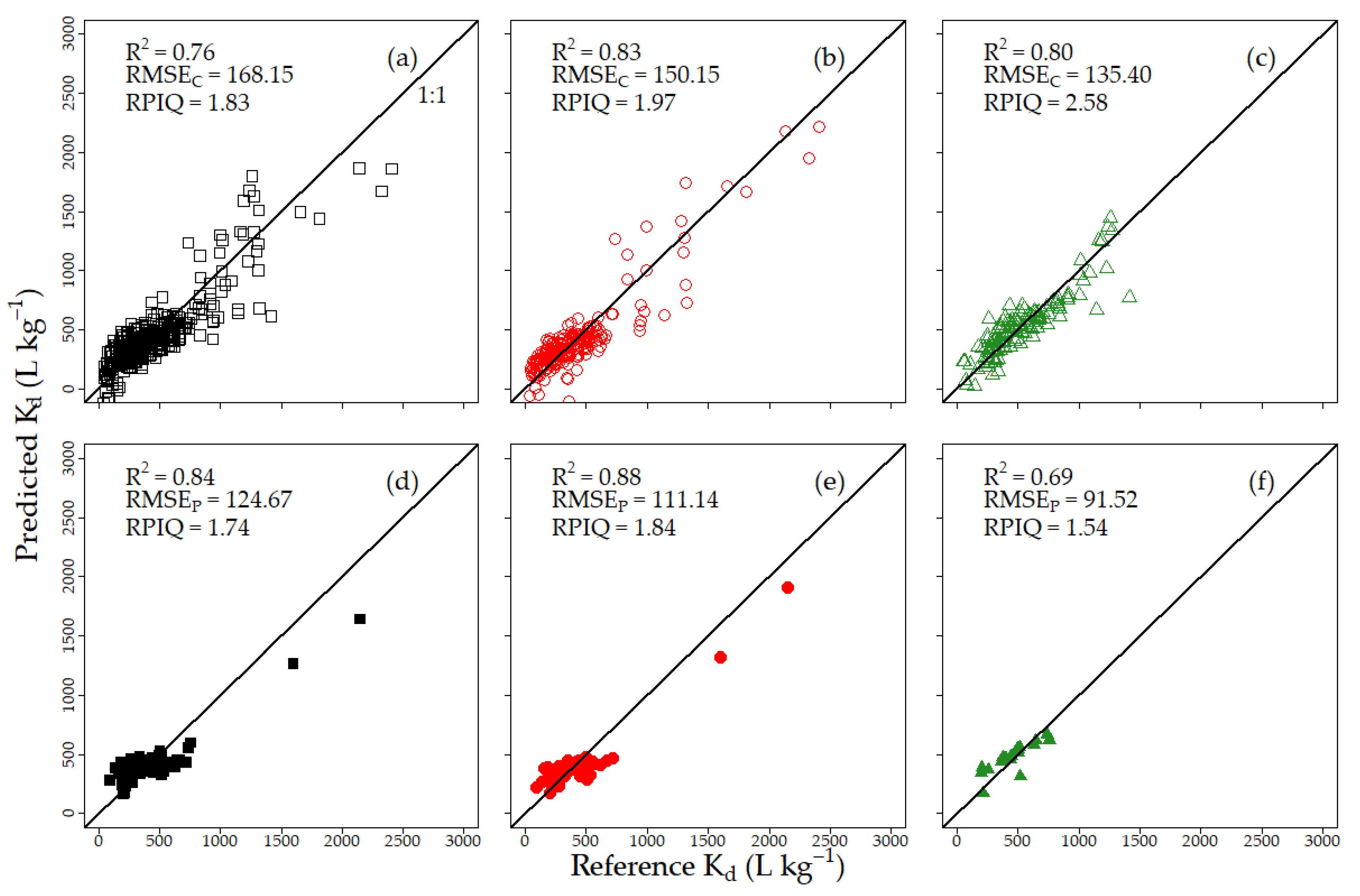
3.2.1. Pedotransfer Functions

The forward stepwise MLR analysis, including all soil samples for the present study, revealed that Fe_ox had the highest contribution, followed by P_ox, TOC, pH, sand, and EC to predict the K_d of glyphosate (

Table A2. Results for the forward stepwise MLR analysis to predict the K_d (L kg⁻¹) of glyphosate with all samples for each dataset.

All Samples of the Combined Dataset			All Samples of the Danish Dataset			All Samples of the Greenlandic Dataset
Variables	R2 a	RMSE b	Variables	R2 a	RMSE b	Variables	R2 a	RMSE b
Constant		329.73	Constant		343.52	Constant		284.81
Feox	0.59	211.29	Feox	0.61	214.36	Feox	0.56	188.76
Pox	0.64	197.25	Pox	0.71	186.94	Pox	0.71	154.84
TOC	0.72	176.07	TOC	0.78	161.01	Sand	0.79	132.69
pH	0.73	170.73	EC	0.82	148.45	Alox	0.80	129.77
Sand	0.77	160.02	pH	0.83	141.70	pH	0.81	128.07
EC	0.78	156.56	Clay	0.84	139.71

^a R², coefficient of determination; ^b RMSE, root mean square error.

—see Appendix A). However, including EC in the MLR model did not improve the model accuracy significantly. The contribution of other soil properties was not significant at p < 0.05. Hence, the K_d was predicted using Fe_ox, P_ox, TOC, pH, and sand with an R² = 0.77 and RMSE_C = 160.02 L kg⁻¹ for all samples. The general PTF developed on all samples is as follows, where the contribution of all variables was significant at p < 0.001:

K_d = 1529.82 − (5.95 × sand) + (57.75 × TOC) − (132.03 × pH) + (4.71 × Fe_ox) − (13.74 × P_ox)

(3)

The summary of the forward stepwise MLR analysis for the combined, DK, and GR calibration subsets is presented in

Table 2. Summary of the forward stepwise multiple linear regression (MLR) analysis to predict the K_d (L kg⁻¹) when more and more soil properties are added one by one. The MLR model statistics are shown for the calibration subset of each dataset.

Combined			Denmark			Greenland
Variables	R2 a	RMSEC b	Variables	R2 a	RMSEC b	Variables	R2 a	RMSEC b
Constant		344.00	Constant		358.29	Constant		298.92
Feox	0.59	220.15	Feox	0.61	225.18	Feox	0.57	197.24
Pox	0.64	206.68	Pox	0.70	197.36	Pox	0.72	159.21
TOC	0.71	185.21	TOC	0.78	169.07	Sand	0.79	138.13
pH	0.73	179.16	EC	0.81	156.71	Alox	0.80	135.40
Sand	0.76	168.15	pH	0.83	150.15	pH	0.81	133.56
EC	0.77	164.92	Clay	0.84	147.63

^a R², coefficient of determination for the calibration subsets; ^b RMSE_C, root mean square error for the calibration subsets.

. The performance of PTF for the combined calibration subset (Table 2) was nearly the same as the PTF developed on all samples (Table A2—see Appendix A). For the DK calibration subset, the glyphosate K_d can be predicted from the linear combination of all soil properties except silt, sand, and Al_ox (not significant at p < 0.05). However, adding clay into the PTF did not improve prediction accuracy significantly because RMSE_C values only decreased by 1.6% if clay was included in the PTF for the DK calibration subset (Table 2). Soil properties such as clay, silt, TOC, and EC were not significant (at p < 0.05) in terms of predicting the K_d of glyphosate for the GR calibration subset. Furthermore, pH was removed due to not improving the performance of PTF significantly for the GR soils.

The PTFs for all three calibration subsets are provided in

Table A3. Pedotransfer functions to predict the K_d (L kg⁻¹) of glyphosate for all the calibration subsets.

Dataset	PTFs
Combined calibration subset	Kd a = 1524.34 − (5.87 × sand) + (55.62 × TOC b) − (131.54 × pH) + (4.56 × Feox c) − (13.39 × Pox c)
Danish calibration subset	Kd = 761.25 + (76.46 × TOC) − (78.32 × pH) − (129.20 × EC d) + (7.46 × Feox) − (20.70 × Pox)
Greenlandic calibration subset	Kd = 1521.14 − (11.53 × sand) + (3.12 × Feox) + (2.82 × Alox c) − (17.52 × Pox)

^a K_d, soil sorption coefficient of glyphosate; ^b TOC, total organic carbon; ^c Fe_ox, Al_ox, and P_ox, oxalate-extractable iron, aluminum, and phosphorous; ^d EC, electrical conductivity; all soil properties are significant at p < 0.001 except Al_ox in the Greenlandic dataset (p < 0.05).

. The highest contributing two soil properties (Fe_ox and P_ox) in PTF were the same for all datasets (Table 2). Additionally, the third highest contributor was TOC for all datasets except the GR dataset (Table 2), which also agrees with the findings of the single linear regression model (see previous section).

The PTF generated from the calibration subset of each dataset was used for validation (Figure 5). The DK and GR calibration PTFs performed better than the combined calibration PTF (RPIQ = 1.97, 2.58, and 1.83, respectively). However, GR validation PTFs had the lowest RPIQ among all validation PTFs. Two samples with the highest K_d values influenced the combined and DK validation PTFs’ performance (Figure 5d,e). The R² and RMSE_P values decreased, and RPIQ increased when those two extreme samples were removed from the two above-mentioned PTFs. As an example, R², RMSE_P, and RPIQ shifted from 0.84 to 0.45, 124.67 to 107.64 L kg⁻¹, and 1.74 to 2.02, respectively, when those two extreme samples were removed from the combined validation PTF.

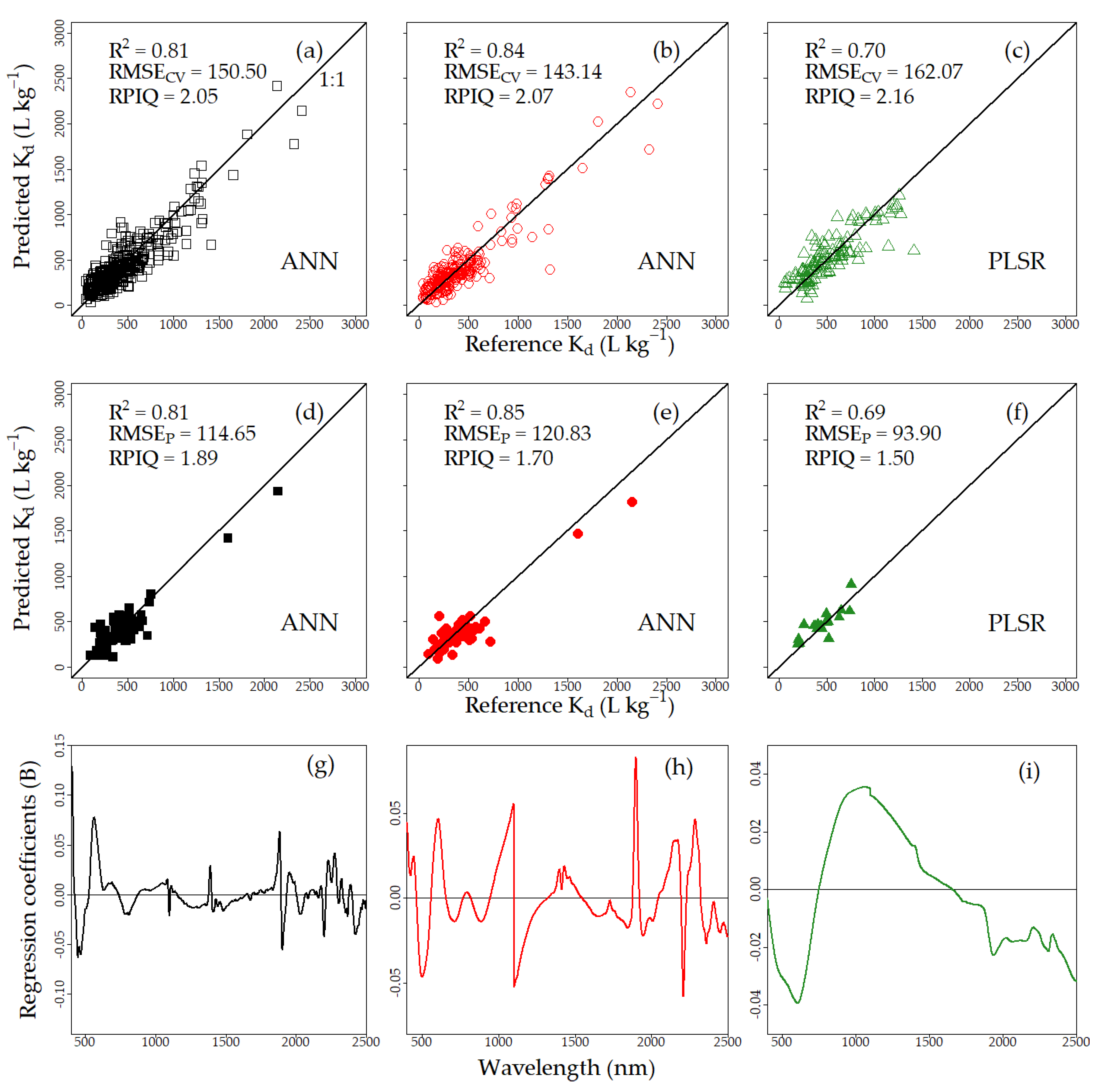
3.2.2. Spectral Model

While developing the vis–NIRS models, the effect of spectral pre-processing techniques on both the PLSR and ANN calibration models was evaluated in comparison with the respective model’s performance on raw spectra (

Table 3. The effect of spectral pre-processing on partial least squares regression (PLSR) and artificial neural network (ANN) calibration models of each dataset to predict the K_d of glyphosate.

Pre-Processing Technique	No of LVs a	R2 b	RMSECV cin L kg−1	RPIQ d
Combined dataset (n = 351)
No pre-processing	14	0.66 e (0.81 f)	199.52 (150.50)	1.54 (2.05)
SNV g	13	0.57 (0.70)	234.29 (189.83)	1.31 (1.62)
MSC h	11	0.57 (0.68)	226.18 (198.45)	1.36 (1.55)
SG 1st derivative i	11	0.69 (0.79)	193.09 (158.30)	1.60 (1.95)
SG 2nd derivative i	11	0.62 (0.76)	211.80 (166.83)	1.45 (1.85)
SG 1st derivative + MSC	11	0.64 (0.74)	206.82 (176.67)	1.49 (1.74)
SG 1st derivative + SNV	13	0.73 (0.77)	182.44 (164.52)	1.69 (1.87)
Danish dataset (n = 228)
No pre-processing	15	0.80 (0.84)	162.44 (143.14)	1.82 (2.07)
SNV	14	0.70 (0.80)	201.36 (163.55)	1.47 (1.81)
MSC	15	0.78 (0.80)	168.68 (157.71)	1.75 (1.88)
SG 1st derivative	10	0.77 (0.82)	172.19 (151.87)	1.72 (1.95)
SG 2nd derivative	11	0.77 (0.83)	173.63 (145.63)	1.70 (2.05)
SG 1st derivative + MSC	12	0.74 (0.82)	182.39 (151.72)	1.62 (1.95)
SG 1st derivative + SNV	09	0.64 (0.77)	221.55 (173.55)	1.34 (1.71)
Greenlandic dataset (n = 123)
No pre-processing	03	0.70 (0.68)	162.07 (168.14)	2.16 (2.08)
SNV	07	0.66 (0.63)	183.60 (183.23)	1.91 (1.91)
MSC	03	0.48 (0.46)	215.18 (218.69)	1.63 (1.60)
SG 1st derivative	03	0.66 (0.66)	173.78 (173.84)	2.01 (2.01)
SG 2nd derivative	04	0.70 (0.69)	162.99 (166.52)	2.15 (2.10)
SG 1st derivative + MSC	04	0.59 (0.59)	191.90 (190.71)	1.82 (1.84)
SG 1st derivative + SNV	03	0.67 (0.68)	172.63 (171.70)	2.03 (2.04)

^a LVs, latent variables; ^b R², coefficient of determination for cross-validation; ^c RMSE_CV, root mean square error for cross-validation; ^d RPIQ, ratio of performance to interquartile range for cross-validation; ^e PLSR model results; ^f ANN model results; ^g SNV, standard normal variate; ^h MSC, multiple scatter correction; ⁱ SG 1st and 2nd derivative, Savitzky–Golay 1st and 2nd derivative.

). For the combined dataset, the best PLSR model was obtained for the SG 1st derivative + SNV pretreatment with a reduction of 9% RMSE_CV compared to the model based on raw spectra. On the contrary, the ANN model performed the best on raw spectra compared to the pre-processed spectra. The application of spectral pre-processing on the DK calibration subset did not improve the model’s accuracy, and thus, the best PLSR and ANN models were obtained on raw DK spectra. However, the pre-processing techniques helped to reduce model complexity by decreasing the number of LVs (except MSC) for the DK set. For the GR calibration subset, the best PLSR model was obtained on raw spectra. Although the SG 2nd derivative pretreatment slightly improved the ANN model of the GR calibration subset compared to the model developed on the raw spectra, it increased the number of LVs by 1. Therefore, the ANN model developed on raw spectra was considered the best ANN model for the GR set. The use of ANN resulted in improved calibration models for the combined and the DK sets. On the contrary, a slightly better performance of PLSR over ANN was reported for the GR calibration subset. As mentioned above, the optimal number of LVs was different depending on the dataset and pretreatment. In general, higher LVs were selected for the combined and the DK models. This is a result of the higher variability of these two types of sets as compared to the GR dataset, which is much more local.

The robustness of the best PLSR and ANN calibration models obtained for each dataset was tested further with the validation subsets (

Table A4. The summary of validation results for the best PLSR and ANN calibration models of each dataset.

Dataset	No of LVs a	R2 b	RMSEP c in L kg−1	RPIQ d
Combined	13 e (14 f)	0.69 (0.81)	162.01 (114.65)	1.34 (1.89)
Denmark	15 (15)	0.82 (0.85)	130.12 (120.83)	1.58 (1.70)
Greenland	03 (04)	0.69 (0.62)	93.90 (97.98)	1.50 (1.44)

^a LVs, latent variables; ^b R², coefficient of determination for validation subset; ^c RMSE_P, root mean square error for prediction; ^d RPIQ, ratio of performance to interquartile range; ^e PLSR model results; ^f ANN model results.

—see Appendix A). The ANN validation model outperformed the PLSR validation model for both the combined and DK datasets. However, the ANN validation model resulted in a higher reduction of standard error from the respective PLSR validation models for the combined dataset (29%) than the DK dataset (7%). In contrast, higher accuracy was obtained for the PLSR than the ANN validation model (R² = 0.69 and RMSE_P = 93.90 L kg⁻¹ for PLSR while R² = 0.62, RMSE_P = 97.98 L kg⁻¹ for ANN) of the GR dataset. Figure 6 shows the output of calibration models (spectral models that generated the highest prediction accuracy) with their respective regression coefficient plots and validation results of each dataset.

The combined validation model predicted the glyphosate K_d more accurately than the DK validation model (Figure 6d,e). The presence of two samples with the highest K_d values in the combined and DK validation subsets (Figure 6d,e) had a clear influence on the validation models’ performance, similar to PTF. The GR validation model resulted in the lowest predictive ability of all three models when comparing RPIQ values.

The RC plot of a vis–NIRS model exhibits important wavelengths for predicting a specific independent variable [58]. The RC graphs are extracted from the PLSR models as spectra compression with PLSR was performed prior to each ANN analysis. For example, the best spectral model of the combined dataset was the ANN model developed on the raw spectra. Hence, the RC of the combined dataset was shown for the PLSR model developed on the raw spectra (Figure 6g). The combined RC plot depicted peaks around 410, 450, 470, 580, and 800 nm in the visible region and peaks around 1100, 1390, 1885, 1900, 2020, 2200, 2290, and 2400 nm in the NIR region of the electromagnetic spectrum (Figure 6g). The RC plot of the DK model exhibited a few prominent peaks in the visible region around 450, 500, and 610 nm and prominent peaks in the NIR region around 1100, 1900, 2200, and 2290 nm (Figure 6h). Unlike the combined and DK plots, the RC plot of the GR dataset demonstrated broad absorption peaks in the visible region near 600 and 900 nm (Figure 6i).

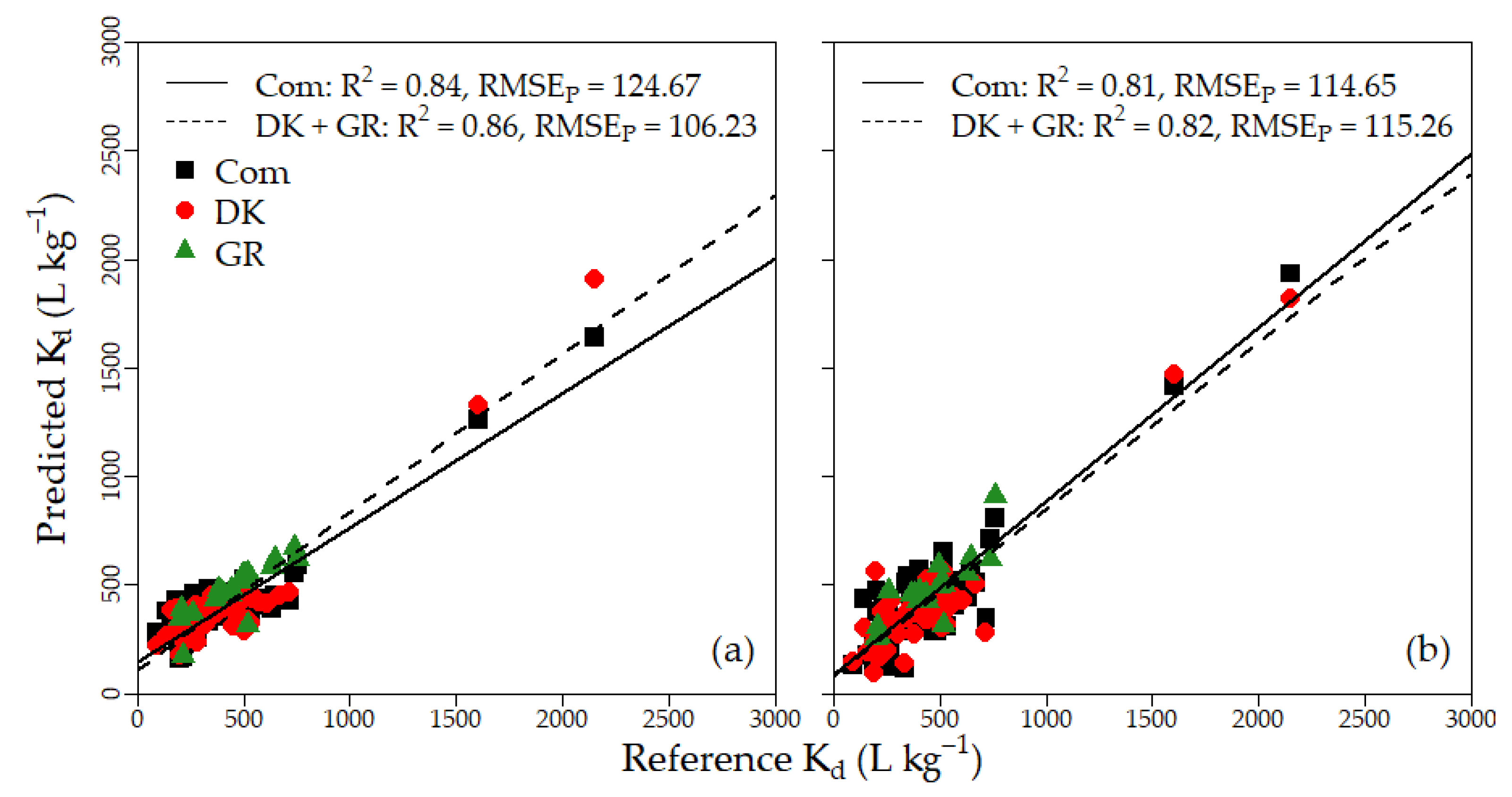
3.2.3. Assessing the Advantages of Developing Individual Models

The K_d values estimated by the individual validation models were joined together. For the PTFs, the recalculated error of the joint set indicated that the RMSE_p for the K_d of glyphosate improved when using prediction values from the individual models rather than the combined model (Figure 7a). However, the Mann–Whitney rank sum test indicated that the accuracy of the estimated K_d of glyphosate by the individual models pulled together was not significantly different from the accuracy of the combined model for PTFs. Likewise, the individual vis–NIRS models together generated almost similar RMSE_P to the combined vis–NIRS model (Figure 7b). Moreover, the differences in prediction accuracy between the combined and joint individual vis–NIRS models were not significant (p = 0.14).

4. Discussion

4.1. Evaluation of Exploratory Analysis Results

The descriptive statistics of soil properties depicted that the calibration subset represented the entire dataset well covering the full range of soil properties (Table 1). This was found to be true for all three datasets. The output of spectral responses and score plots (Figure 3a,c) also agrees with the above finding. Interestingly, spectra for almost all the GR samples overlapped with the DK soil spectra (Figure 3b), and the scores of most of the GR samples overlapped with the scores of DK samples (Figure 3d). The most plausible explanation for that overlap can be the similarities in mineralogical characteristics for those DK and GR soil samples.

The SLR analysis showed that Fe_ox had the highest correlation with K_d for all datasets (Figure 4). Likewise, other studies have reported amorphous iron oxide as an important sorbent of glyphosate [21,59,60]. Sprankle et al. [61] reported the affinity of glyphosate to clay. However, clay was not found to be an important predictor of K_d for each of the datasets, which can be a consequence of the strong correlation between clay and sand (Table A2—see Appendix A). Piccolo et al. [18] reported that glyphosate could be adsorbed in humic extracts. The soil organic fractions could explain the variation of glyphosate K_d for all datasets except the GR dataset (Figure 4). Since the turnover and mineralization of organic matter in GR is less advanced, organic matter was expected to hold fewer sorption sites available to glyphosate, which was considered a possible reason for having no significant correlation of TOC with K_d.

4.2. Evaluation of K_d Predictions by PTF and Vis–NIRS

The best five (combined and DK) or best four (GR) parameters were used to produce an acceptable PTF prediction of glyphosate K_d (Table 2 and Table A3). Developing simple PTF with easily measurable two or three parameters is out of this study’s scope. However, an overview of the performance of PTF with easily measurable soil properties to predict the glyphosate K_d can be found in Table 2. For example, K_d can be predicted with an R² = 0.64 and RMSE_C = 206.68 L kg⁻¹ using only Fe_ox and P_ox for the combined calibration subset (Table 2). Interestingly, P_ox was the second most important predictor in PTFs (Table 2) despite its weak correlation to K_d for both the combined and DK calibration subsets (Table A1). The P_ox was also found to be a controlling factor for the variation in the K_d of glyphosate, together with Al_ox and pH, in acidic soils of New Zealand [34]. Soil properties such as TOC and Fe_ox had significant contributions to predicting K_d (Table 2 and Figure 4) for the combined and DK calibration subsets. The correlation of P_ox with those two above-mentioned soil properties (Table A1) might be responsible for the contribution of P_ox to predict K_d for the combined and DK calibration PTFs. Other studies have also reported the significant contribution of Fe_ox [24,34,62] and OC [63] for phosphorus retention in soil.

The effect of pre-processing on vis–NIRS calibration models differed depending on the dataset and modeling technique applied (Table 3). Improved model results after the application of pre-processing were reported only for the combined dataset modeled with PLSR. The applied pre-processing techniques included the 1st derivative and standard normal variate, which correct for baseline effects in spectra for the purpose of removing nonchemical effects and removing multiplicative interferences of scatter and particle size effects from spectral data, respectively [51]. Hermansen et al. [34] also reported improved PLSR results for K_d after the application of spectral pretreatments (2nd derivative) for a heterogenous dataset from New Zealand. In line with our findings, Paradelo et al. [30] did not improve the calibration results by applying pretreatment to their dataset collected from a single field. This indicates that the ANN technique can account for both baseline and multiplicative interferences present in the dataset representing a mixture of soil samples affected by different forming factors related to the geographic origin.

Likewise, the ANN method worked best for the combined and DK dataset, whereas PLSR provided the best estimations of K_d for the GR set. This is in line with the previous argumentation. The GR set is smaller, more homogenous, and consists of normally distributed data from four fields only; thus, the best results with the linear PLSR. In turn, the more complex models based on the combined and the DK sets required the application of the ANN technique.

The sorption coefficient for glyphosate is not a spectrally active soil component. It is, therefore, interesting to understand which wavelengths contribute to explaining its variability. In the combined RC plot (Figure 6g), the peaks in the visible region can be associated with the electronic transitions of iron oxides (e.g., the absorption band for goethite: 409, 427, 480, and 490 nm and for hematite: 510, 531, 620 nm) [57,64] or OM (the absorption band for OM: 570–700 nm and for C–H: 825 nm) [55,65,66]. Similar spectral regions (400–700 nm) were selected in the K_d calibration model by Paradelo et al. [30] and Hermansen et al. [34]. The peaks in the NIR region can be assigned to the absorptions of molecular O–H bonds or O–H bonds inside mineral lattice or O–H bonds with metal oxides (near 1400, 1900, 2200 nm) and C–H bonds (near 2400 nm) [56,65,66,67]. The peaks near 1400 and 1900 nm were also reported in the K_d models by Paradelo et al. [30], whereas Hermansen et al. [39] also found the spectral range between 2160 and 2240 nm import in their K_d calibration model. In the DK model, the few prominent peaks in the visible region (Figure 6h) might be associated with the presence of iron oxides [28,64], and the prominent peaks in the NIR region might be indicative of clay mineralogy [27,28,66]. The broad absorption peaks in the visible region (Figure 6i) can be assigned to iron oxides or OM for the GR samples [55,57,64]. The important wavelengths used in the developed models and as indicated by the RC are aligned with the existing knowledge on glyphosate and its behavior in soils as well as the results from the developed PTFs. The vis–NIRS models of glyphosate K_d rely on the spectrally active components which glyphosate is known to have a high affinity for, such as iron oxides and clay minerals [9,10,16,17,21,22]. Thus, the presence of peaks in the visible range and in the regions typical for OH bonds in the RC of all three calibration models. Moreover, the peaks assigned to SOM in the combined and the DK model confirm that the prediction of K_d additionally relies on spectrally active humic substances to which glyphosate can adsorb [18].

The prediction accuracy obtained for the best vis–NIRS model was higher than the PTF for the combined dataset, while this was not the case for the DK and GR models. However, the results of those two approaches were not significantly different (p > 0.1, according to the Mann–Whitney rank sum test) for each dataset, and thus, may also be attributed to random errors. The calibration results presented here show similar yet a bit higher predictive ability than those in the regional scale study by Hermansen et al. [34]. In our study, the RPIQ values for all three models were >2.05, whereas Hermansen et al. [34] obtained an RPIQ of 1.79 for the cross-validation PLSR model of glyphosate K_d. On the contrary, a higher accuracy than in our study was reported by Paradelo et al. [30] (RPIQ = 2.7) and can be attributed to a much lower variability because of utilizing data from one field only.

5. Conclusions

The study investigated the potential of vis–NIRS to predict the soil sorption coefficient (K_d) of glyphosate in comparison to PTF for Danish (DK) and southwest Greenlandic (GR) soils. The nature of the dataset allowed us to investigate the effects of developing a combined calibration model containing the DK and GR samples as well as two models dedicated to the two geographic origins and test their robustness using a prediction set. We obtained successful estimates for glyphosate K_d and found that the K_d for the DK and GR soils can be predicted from the combined model as accurately as the individual models. This implies no need to develop individual models representative of one country or a specific parent material. The comparison of linear (PLSR) and non-linear (ANN) techniques for K_d modeling revealed that PLSR can be used for smaller and more homogenous datasets, whereas in the case of datasets combining samples from several geographic origins, the application of ANN for K_d estimation is more advantageous. Moreover, when applying ANN to such a complex dataset, there is no need to apply pre-processing techniques accounting for both physical and chemical interferences. Finally, the predictive ability of the glyphosate K_d for vis–NIRS models was statistically insignificantly lower compared to PTFs.

Considering the multiple advantages of vis–NIRS, such as short measurement time, little sample preparation, and the possibility to analyze several soil properties simultaneously, including those needed for the development of PTFs, this technique appears to be a great alternative to the PTF for the estimation of glyphosate K_d.

However, as the performance of vis–NIRS is dataset dependent, these results may not be valid for other countries with more pronounced differences in soil types, parent material, and mineralogy. Further studies incorporating soil samples from several countries should be conducted to confirm our findings, and the possibility of using satellite imaging data to cover larger scales should be tested.

References

1. De Gerónimo, E.; Aparicio, V.C.; Costa, J.L. Glyphosate sorption to soils of Argentina. Estimation of affinity coefficient by pedotransfer function. Geoderma 2018, 322, 140–148. [Google Scholar] [CrossRef]
2. Duke, S.O. The history and current status of glyphosate. Pest Manag. Sci. 2018, 74, 1027–1034. [Google Scholar] [CrossRef] [PubMed]
3. Duke, S.O.; Powles, S.B. Glyphosate: A once-in-a-century herbicide. Pest Manag. Sci. 2008, 64, 319–325. [Google Scholar] [CrossRef] [PubMed]
4. Mensink, H.; Janseen, P. (Eds.) Environmental Health Criteria. In Glyphosate; World Health Organization: Geneva, Switzerland, 1994; ISBN 978-92-4-157159-3. [Google Scholar]
5. Szekacs, A.; Darvas, B. Forty Years with Glyphosate. In Herbicides—Properties, Synthesis and Control of Weeds; Hasaneen, M.N., Ed.; InTech: London, UK, 2012; ISBN 978-953-307-803-8. [Google Scholar]
6. Cheah, U.B.; Kirkwood, R.C.; Lum, K.Y. Adsorption, desorption and mobility of four commonly used pesticides in Malaysian agricultural soils. Pestic. Sci. 1997, 50, 53–63. [Google Scholar] [CrossRef]
7. de Jonge, L.W.; Kjaergaard, C.; Moldrup, P. Colloids and colloid-facilitated transport of contaminants in soils: An introduction. Vadose Zone J. 2004, 3, 321–325. [Google Scholar] [CrossRef] [Green Version]
8. Norgaard, T.; Moldrup, P.; Ferré, T.P.A.; Olsen, P.; Rosenbom, A.E.; de Jonge, L.W. Leaching of glyphosate and aminomethylphosphonic acid from an agricultural field over a twelve-year period. Vadose Zone J. 2014, 13, vzj2014.05.0054. [Google Scholar] [CrossRef]
9. Vereecken, H. Mobility and leaching of glyphosate: A review. Pest Manag. Sci. 2005, 61, 1139–1151. [Google Scholar] [CrossRef]
10. Borggaard, O.K.; Gimsing, A.L. Fate of glyphosate in soil and the possibility of leaching to ground and surface waters: A review. Pest Manag. Sci. 2008, 64, 441–456. [Google Scholar] [CrossRef]
11. Farenhorst, A.; Papiernik, S.K.; Saiyed, I.; Messing, P.; Stephens, K.D.; Schumacher, J.A.; Lobb, D.A.; Li, S.; Lindstrom, M.J.; Schumacher, T.E. Herbicide sorption coefficients in relation to soil properties and terrain attributes on a cultivated prairie. J. Environ. Qual. 2008, 37, 1201–1208. [Google Scholar] [CrossRef] [Green Version]
12. Farenhorst, A.; McQueen, D.A.R.; Saiyed, I.; Hilderbrand, C.; Li, S.; Lobb, D.A.; Messing, P.; Schumacher, T.E.; Papiernik, S.K.; Lindstrom, M.J. Variations in soil properties and herbicide sorption coefficients with depth in relation to PRZM (pesticide root zone model) calculations. Geoderma 2009, 150, 267–277. [Google Scholar] [CrossRef]
13. Gevao, B.; Semple, K.T.; Jones, K.C. Bound pesticide residues in soils: A review. Environ. Pollut. 2000, 108, 3–14. [Google Scholar] [CrossRef] [PubMed]
14. Wauchope, R.D.; Yeh, S.; Linders, J.B.H.J.; Kloskowski, R.; Tanaka, K.; Rubin, B.; Katayama, A.; Kördel, W.; Gerstl, Z.; Lane, M.; et al. Pesticide soil sorption parameters: Theory, measurement, uses, limitations and reliability. Pest Manag. Sci. 2002, 58, 419–445. [Google Scholar] [CrossRef] [PubMed]
15. Ololade, I.A.; Oladoja, N.A.; Oloye, F.F.; Alomaja, F.; Akerele, D.D.; Iwaye, J.; Aikpokpodion, P. Sorption of glyphosate on soil components: The roles of metal oxides and organic materials. Soil Sediment Contam. Int. J. 2014, 23, 571–585. [Google Scholar] [CrossRef]
16. Dollinger, J.; Dagès, C.; Voltz, M. Glyphosate sorption to soils and sediments predicted by pedotransfer functions. Environ. Chem. Lett. 2015, 13, 293–307. [Google Scholar] [CrossRef]
17. Morillo, E.; Undabeytia, T.; Maqueda, C.; Ramos, A. Glyphosate adsorption on soils of different characteristics. Influence of copper addition. Chemosphere 2000, 40, 103–107. [Google Scholar] [CrossRef]
18. Piccolo, A.; Celano, G.; Conte, P. Adsorption of glyphosate by humic substances. J. Agric. Food Chem. 1996, 44, 2442–2446. [Google Scholar] [CrossRef]
19. Arroyave, J.M.; Waiman, C.C.; Zanini, G.P.; Avena, M.J. Effect of humic acid on the adsorption/desorption behavior of glyphosate on goethite. Isotherms and kinetics. Chemosphere 2016, 145, 34–41. [Google Scholar] [CrossRef]
20. Day, G.M.; Hart, B.T.; McKelvie, I.D.; Beckett, R. Influence of natural organic matter on the sorption of biocides onto goethite, II. Glyphosate. Environ. Technol. 1997, 18, 781–794. [Google Scholar] [CrossRef]
21. de Jonge, H.; de Jonge, L.W.; Jacobsen, O.H.; Yamaguchi, T.; Moldrup, P. Glyphosate sorption in soils of different pH and phosphorus content. Soil Sci. 2001, 166, 230–238. [Google Scholar] [CrossRef]
22. de Jonge, H.; de Jonge, L.W. Influence of pH and solution composition on the sorption of glyphosate and prochloraz to a sandy loam soil. Chemosphere 1999, 39, 753–763. [Google Scholar] [CrossRef]
23. Gimsing, A.L.; Borggaard, O.K.; Bang, M. Influence of soil composition on adsorption of glyphosate and phosphate by contrasting Danish surface soils. Eur. J. Soil Sci. 2004, 55, 183–191. [Google Scholar] [CrossRef]
24. Paradelo, M.; Norgaard, T.; Moldrup, P.; Ferré, T.P.A.; Kumari, K.G.I.D.; Arthur, E.; de Jonge, L.W. Prediction of the glyphosate sorption coefficient across two loamy agricultural fields. Geoderma 2015, 259–260, 224–232. [Google Scholar] [CrossRef]
25. Bellon-Maurel, V.; McBratney, A. Near-infrared (NIR) and mid-infrared (MIR) spectroscopic techniques for assessing the amount of carbon stock in soils—Critical review and research perspectives. Soil Biol. Biochem. 2011, 43, 1398–1410. [Google Scholar] [CrossRef]
26. Rossel, R.A.V.; Walvoort, D.J.J.; McBratney, A.B.; Janik, L.J.; Skjemstad, J.O. Visible, near infrared, mid infrared or combined diffuse reflectance spectroscopy for simultaneous assessment of various soil properties. Geoderma 2006, 131, 59–75. [Google Scholar] [CrossRef]
27. Soriano-Disla, J.M.; Janik, L.J.; Viscarra Rossel, R.A.; Macdonald, L.M.; McLaughlin, M.J. The performance of visible, near-, and mid-infrared reflectance spectroscopy for prediction of soil physical, chemical, and biological properties. Appl. Spectrosc. Rev. 2014, 49, 139–186. [Google Scholar] [CrossRef]
28. Stenberg, B.; Viscarra Rossel, R.A.; Mouazen, A.M.; Wetterlind, J. Visible and near infrared spectroscopy in soil science. In Advances in Agronomy; Elsevier: Amsterdam, The Netherlands, 2010; Volume 107, pp. 163–215. ISBN 978-0-12-381033-5. [Google Scholar]
29. Ben-Dor, E. Quantitative remote sensing of soil properties. In Advances in Agronomy; Elsevier: Amsterdam, The Netherlands, 2002; Volume 75, pp. 173–243. ISBN 978-0-12-000793-6. [Google Scholar]
30. Paradelo, M.; Hermansen, C.; Knadel, M.; Moldrup, P.; Greve, M.H.; de Jonge, L.W. Field-scale predictions of soil contaminant sorption using visible–near infrared spectroscopy. J. Infrared Spectrosc. 2016, 24, 281–291. [Google Scholar] [CrossRef]
31. Horta, A.; Malone, B.; Stockmann, U.; Minasny, B.; Bishop, T.F.A.; McBratney, A.B.; Pallasser, R.; Pozza, L. Potential of integrated field spectroscopy and spatial analysis for enhanced assessment of soil contamination: A prospective review. Geoderma 2015, 241–242, 180–209. [Google Scholar] [CrossRef] [Green Version]
32. Goldshleger, N.; Chudnovsky, A.; Ben-Dor, E. Using reflectance spectroscopy and artificial neural network to assess water infiltration rate into the soil profile. Appl. Environ. Soil Sci. 2012, 2012, 439567. [Google Scholar] [CrossRef] [Green Version]
33. Janik, L.J.; Forrester, S.T.; Rawson, A. The prediction of soil chemical and physical properties from mid-infrared spectroscopy and combined partial least-squares regression and neural networks (PLS-NN) analysis. Chemom. Intell. Lab. Syst. 2009, 97, 179–188. [Google Scholar] [CrossRef]
34. Hermansen, C.; Norgaard, T.; Wollesen de Jonge, L.; Moldrup, P.; Müller, K.; Knadel, M. Predicting glyphosate sorption across New Zealand pastoral soils using basic soil properties or vis–NIR spectroscopy. Geoderma 2020, 360, 114009. [Google Scholar] [CrossRef]
35. Vaudour, E.; Gomez, C.; Fouad, Y.; Lagacherie, P. Sentinel-2 Image Capacities to Predict Common Topsoil Properties of Temperate and Mediterranean Agroecosystems. Remote Sens. Environ. 2019, 223, 21–33. [Google Scholar] [CrossRef]
36. Ge, Y.; Thomasson, J.A.; Sui, R. Remote Sensing of Soil Properties in Precision Agriculture: A Review. Front. Earth Sci. 2011, 5, 229–238. [Google Scholar] [CrossRef]
37. Yu, H.; Kong, B.; Wang, Q.; Liu, X.; Liu, X. Hyperspectral Remote Sensing Applications in Soil: A Review. In Hyperspectral Remote Sensing; Elsevier: Amsterdam, The Netherlands, 2020; pp. 269–291. ISBN 978-0-08-102894-0. [Google Scholar]
38. Ben-Dor, E.; Chabrillat, S.; Demattê, J.A.M.; Taylor, G.R.; Hill, J.; Whiting, M.L.; Sommer, S. Using Imaging Spectroscopy to Study Soil Properties. Remote Sens. Environ. 2009, 113, S38–S55. [Google Scholar] [CrossRef]
39. Xiao, W.; Zhang, Y.; Wang, H.; Li, F.; Jin, H. Heterogeneous Knowledge Distillation for Simultaneous Infrared-Visible Image Fusion and Super-Resolution. IEEE Trans. Instrum. Meas. 2022, 71, 5004015. [Google Scholar] [CrossRef]
40. Wang, P.; Wang, L.; Leung, H.; Zhang, G. Super-Resolution Mapping Based on Spatial–Spectral Correlation for Spectral Imagery. IEEE Trans. Geosci. Remote Sens. 2021, 59, 2256–2268. [Google Scholar] [CrossRef]
41. Breuning-Madsen, H.; Jensen, N.H. Soil map of Denmark according to the revised FAO legend 1990. Geogr. Tidsskr.-Dan. J. Geogr. 1996, 96, 51–59. [Google Scholar] [CrossRef]
42. Moberg, J.P. Composition and development of the clay fraction in Danish soils. An overview/Composition et évolution de la fraction argileuse des sols danois. Un Aperçu. Sci. Géologiques Bull. Mémoires 1990, 43, 193–202. [Google Scholar] [CrossRef]
43. Garde, A.A.; Hamilton, M.A.; Chadwick, B.; Grocott, J.; McCaffrey, K.J. The Ketilidian orogen of South Greenland: Geochronology, tectonics, magmatism, and fore-arc accretion during Palaeoproterozoic oblique convergence. Can. J. Earth Sci. 2002, 39, 765–793. [Google Scholar] [CrossRef]
44. Ogrič, M.; Knadel, M.; Kristiansen, S.M.; Peng, Y.; De Jonge, L.W.; Adhikari, K.; Greve, M.H. Soil organic carbon predictions in subarctic Greenland by visible–near infrared spectroscopy. Arct. Antarct. Alp. Res. 2019, 51, 490–505. [Google Scholar] [CrossRef] [Green Version]
45. Gee, G.W.; Or, D. Partcle-Size Analysis. In Methods of Soil Analysis; SSSA: Madison, WI, USA, 2002; pp. 255–293. [Google Scholar]
46. Thomas, G.W. Soil pH and Soil Acidity. In Methods of Soil Analysis; Sparks, D.L., Page, A.L., Helmke, P.A., Loeppert, R.H., Soltanpour, P.N., Tabatabai, M.A., Johnston, C.T., Sumner, M.E., Eds.; SSSA Book Series; Soil Science Society of America, American Society of Agronomy: Madison, WI, USA, 1996; pp. 475–490. ISBN 978-0-89118-866-7. [Google Scholar]
47. Schoumans, O.F.; Breeuwsma, A.; Vries, W.D. Use of soil survey information for assessing the phosphate sorption capacity of heavily manured soils. In Proceedings of the International Conference on Vulnerability of Soil and Groundwater to Pollutants, Amsterdam, The Netherlands, 26–29 October 1987; pp. 1079–1088. [Google Scholar]
48. Soares, A.A.; Moldrup, P.; Minh, L.N.; Vendelboe, A.L.; Schjonning, P.; de Jonge, L.W. Sorption of phenanthrene on agricultural soils. Water Air Soil Pollut. 2013, 224, 1519. [Google Scholar] [CrossRef] [Green Version]
49. Kennard, R.W.; Stone, L.A. Computer aided design of experiments. Technometrics 1969, 11, 137–148. [Google Scholar] [CrossRef]
50. Webster, R.; Oliver, M.A. Geostatistics for Environmental Scientists; John Wiley & Sons: Chichester, UK, 2001. [Google Scholar]
51. Rinnan, Å.; van den Berg, F.; Engelsen, S.B. Review of the most common pre-processing techniques for near-infrared spectra. Trends Anal. Chem. 2009, 28, 1201–1222. [Google Scholar] [CrossRef]
52. Martens, H.; Naes, T. Multivariate Calibration; John Wiley & Sons: New York, NY, USA, 1989. [Google Scholar]
53. Gowen, A.A.; Downey, G.; Esquerre, C.; O’Donnell, C.P. Preventing Over-Fitting in PLS Calibration Models of near-Infrared (NIR) Spectroscopy Data Using Regression Coefficients. J. Chemom. 2011, 25, 375–381. [Google Scholar] [CrossRef]
54. Hecht-Nielsen, R. Neurocomputing; Addison-Wesley: Boston, MA, USA, 1990. [Google Scholar]
55. Galvao, L.S.; Vitorello, I. Role of organic matter in obliterating the effects of iron on spectral reflectance and colour of Brazilian tropical soils. Int. J. Remote Sens. 1998, 19, 1969–1979. [Google Scholar] [CrossRef]
56. Post, J.L.; Nobel, P.N. The near-infrared combination band frequencies of dioctahedral smectites, micas, and illites. Clays Clay Miner. 1993, 41, 639–644. [Google Scholar] [CrossRef]
57. Sherman, D.M.; Waite, T.D. Electronic spectra of Fe3+ oxides and oxide hydroxides in the near IR to near UV. Am. Mineral. 1985, 70, 1262–1269. [Google Scholar]
58. Haaland, D.M.; Thomas, E.V. Partial least-squares methods for spectral analyses. 2. Application to simulated and glass spectral data. Anal. Chem. 1988, 60, 1202–1208. [Google Scholar] [CrossRef]
59. Piccolo, A.; Celano, G.; Arienzo, M.; Mirabella, A. Adsorption and desorption of glyphosate in some European soils. J. Environ. Sci. Health Part B 1994, 29, 1105–1115. [Google Scholar] [CrossRef]
60. Rampazzo, N.; Todorovic, G.R.; Mentler, A.; Blum, W.E.H. Adsorption of glyphosate and aminomethylphosphonic acid in soils. Int. Agrophys. 2013, 27, 203–209. [Google Scholar] [CrossRef]
61. Sprankle, P.; Meggitt, W.F.; Penner, D. Adsorption, mobility, and microbial degradation of glyphosate in the soil. Weed Sci. 1975, 23, 229–234. [Google Scholar] [CrossRef]
62. Freese, D.; Van Der Zee, S.E.A.T.M.; Van Riemsdijk, W.H. Comparison of different models for phosphate sorption as a function of the iron and aluminium oxides of soils. Eur. J. Soil Sci. 1992, 43, 729–738. [Google Scholar] [CrossRef]
63. Ige, D.V.; Akinremi, O.O.; Flaten, D.N. Direct and indirect effects of soil properties on phosphorus retention capacity. Soil Sci. Soc. Am. J. 2007, 71, 95–100. [Google Scholar] [CrossRef] [Green Version]
64. Scheinost, A.C.; Chavernas, A.; Barrón, V.; Torrent, J. Use and limitations of second-derivative diffuse reflectance spectroscopy in the visible to near-infrared range to identify and quantify Fe oxide minerals in soils. Clays Clay Miner. 1998, 46, 528–536. [Google Scholar] [CrossRef]
65. Clark, R.N. Spectroscopy of rocks and minerals, and principles of spectroscopy. In Manual of Remote Sensing, Remote Sensing for the Earth Sciences; Rencz, A.N., Ed.; John Wiley & Sons: New York, NY, USA, 1999; pp. 3–58. [Google Scholar]
66. Clark, R.N.; King, T.V.; Klejwa, M.; Swayze, G.A.; Vergo, N. High spectral resolution reflectance spectroscopy of minerals. J. Geophys. Res. Solid Earth 1990, 95, 12653–12680. [Google Scholar] [CrossRef] [Green Version]
67. Hunt, G.R. Spectral signatures of particulate minerals in the visible and near infrared. Geophysics 1977, 42, 501–513. [Google Scholar] [CrossRef] [Green Version]
Figure 1. Sampling sites of the (a) Danish (DK) and (b) southwest Greenlandic (GR) soils. Red squared area shows the location of four GR fields. Red circle denotes the location of two adjacent fields represented by one location.
Remotesensing 15 01712 g001
Figure 2. A graphical representation of the methodology for predicting the Kd of glyphosate. vis–NIRS, visible near-infrared diffuse reflectance spectroscopy; PTF, pedotransfer function; MLR, multiple linear regression; PLSR, partial least squares regression; ANN, artificial neural network; DK, Denmark; GR, Greenland.
Remotesensing 15 01712 g002
Figure 3. Spectral response for (a) the calibration and validation subsets of the combined dataset and (b) the Danish and Greenlandic datasets; score plots for (c) the calibration and validation subsets of the combined dataset and (d) the Danish and Greenlandic datasets; and (e) loadings plot for all soil samples.
Remotesensing 15 01712 g003
Figure 4. The best three single linear regression models to predict the Kd of glyphosate for the combined (ac), Danish (df), and Greenlandic (gi) datasets. TOC, total organic carbon; Kd, soil sorption coefficient of glyphosate; Feox and Pox, oxalate-extractable iron and phosphorous; R2, coefficient of determination at significance levels of * 0.05, ** 0.01 and *** 0.001; RMSE, root mean square error; Symbology, open symbol represents samples from the calibration subset and closed symbol represents samples from the validation subset for all datasets; Regression line, dashed line for the calibration subset and solid line for the validation subset of each dataset.
Remotesensing 15 01712 g004
Figure 5. Pedotransfer functions for the estimation of the Kd of glyphosate. Results showing the calibration and validation subsets of the combined ((a,d), respectively), Danish ((b,e), respectively), and Greenlandic datasets ((c,f), respectively). R2, coefficient of determination; RMSEC, root mean square error for calibration; RMSEP, root mean square error for prediction; RPIQ, ratio of performance to interquartile range.
Remotesensing 15 01712 g005
Figure 6. Results of the best vis–NIRS calibration and validation models with regression coefficients plot for combined (a,d,g), respectively), Danish (b,e,h), respectively), and Greenlandic (c,f,i), respectively) datasets. ANN, artificial neural network; PLSR, partial least square regression; R2, coefficient of determination; RMSECV, root mean square error for cross-validation; RMSEP, root mean square error for prediction; RPIQ, ratio of performance to interquartile range.
Remotesensing 15 01712 g006
Figure 7. Comparison of the prediction accuracy of the Kd of glyphosate between the combined validation subset and the joint individual validation subsets. Comparison was performed for the (a) PTFs and (b) vis–NIRS models. Com, results from the combined validation model; DK, results from the Danish validation model; GR, results from the Greenlandic validation model.
Remotesensing 15 01712 g007