Article

Evaluation and Error Decomposition of IMERG Product Based on Multiple Satellite Sensors

1
State Key Laboratory of Hydrology-Water Resources and Hydraulic Engineering, Hohai University, Nanjing 210098, China
2
College of Hydrology and Water Resources, Hohai University, Nanjing 210098, China
3
Yangtze Institute for Conservation and Development, Hohai University, Nanjing 210098, China
4
CMA-HHU Joint Laboratory for HydroMeteorological Studies, Hohai University, Nanjing 210098, China
5
Key Laboratory of Water Big Data Technology of Ministry of Water Resources, Hohai University, Nanjing 210098, China
6
Institute for Water and Environmental System Modeling, University of Stuttgart, 70569 Stuttgart, Germany
*
Author to whom correspondence should be addressed.
Remote Sens. 2023, 15(6), 1710; https://doi.org/10.3390/rs15061710
Submission received: 27 February 2023 / Revised: 14 March 2023 / Accepted: 16 March 2023 / Published: 22 March 2023
(This article belongs to the Topic Advanced Research in Precipitation Measurements)

Abstract

:
The Integrated Multisatellite Retrievals for GPM (IMERG) is designed to derive precipitation by merging data from all the passive microwave (PMW) and infrared (IR) sensors. While the input source errors originating from the PMW and IR sensors are important, their structure, characteristics, and algorithm improvement remain unclear. Our study utilized a four-component error decomposition (4CED) method and a systematic and random error decomposition method to evaluate the detectability of IMERG dataset and identify the precipitation errors based on the multi-sensors. The 30 min data from 30 precipitation stations in the Tunxi Watershed were used to evaluate the IMERG data from 2018 to 2020. The input source includes five types of PMW sensors and IR instruments. The results show that the sample ratio for IR (Morph, IR + Morph, and IR only) is much higher than that for PMW (AMSR2, SSMIS, GMI, MHS, and ATMS), with a ratio of 72.8% for IR sources and a ratio of 27.2% for PMW sources. The high false ratio of the IR sensor leads to poor detectability performance of the false alarm ratio (FAR, 0.5854), critical success index (CSI, 0.3014), and Brier score (BS, 0.1126). As for the 4CED, Morph and Morph + IR have a large magnitude of high total bias (TB), hit overestimate bias (HOB), hit underestimate bias (HUB), false bias (FB), and miss bias (MB), which is related to the prediction ability and sample size. In addition, systematic error is the prominent component for AMSR2, SSMIS, GMI, and Morph + IR, indicating some inherent error (retrieval algorithm) that needs to be removed. These findings can support improving the retrieval algorithm and reducing errors in the IMERG dataset.

1. Introduction

Precipitation is an essential hydro-meteorological variable that plays a vital role in the water and energy cycles of the terrestrial ecosystem [1]. Accurate precipitation data with high spatiotemporal resolution are crucial for flood, drought, and water resource management [2,3]. However, obtaining such precipitation data has been a longstanding challenge because of its strong spatiotemporal heterogeneity.
There are three mainstream methods to measure precipitation: rain gauge measurement, radar observation, and satellite retrieval. Each of these methods has different advantages and disadvantages due to the inability to achieve high spatiotemporal resolution and precision. Rain gauge measurement is a traditional and direct method to obtain relatively reliable and high-precision precipitation with a high temporal resolution at a specific point, while it cannot completely cover an area and capture spatial variability [4]. For radar observation, its spatial and temporal resolution is superior to other sensors, but there are several drawbacks, such as non-precipitation radar echoes, radar artifacts, beam blockage, range degradation and earth curvature, non-uniform beam filling, and bright banding. Satellite retrieval has high temporal resolution and global spatial coverage, particularly in remote regions where gauge or radar observation is sparse or nonexistent [5,6].
Satellite precipitation estimates derive from several sensor observations based on different platforms [7,8,9]. Sensor types mainly include infrared (IR) and passive microwave (PMW) sensors. Although IR has a high spatiotemporal resolution, it lacks a physical relationship with rain rates, which is an indirect estimate resulting in the insufficient accuracy of instantaneous precipitation rate [10,11,12]. The PMW can provide more direct precipitation estimates by using a direct physical connection with hydrometeor profiles, while it has sparse time–space sampling [13,14]. Combining the advantages of IR and PMW, several satellite precipitation products (SPPs) have been developed, including the Precipitation Estimation from Remotely Sensed Information using Artificial Neural Networks (PERSIANN) [15], Climate Prediction Center Morphing Technique (CMORPH) [16], Global Satellite Mapping of Precipitation (GSMaP) [17], Tropical Rainfall Measuring Mission (TRMM) Multisatellite Precipitation Analysis (TMPA) [9], and Global Precipitation Measurement (GPM). The Integrated Multisatellite Retrievals for GPM (IMERG) was developed to merge precipitation estimates from passive microwave (PMW), microwave-calibrated infrared (IR) satellite estimates, additional satellite estimates, and precipitation gauge data. First, the PMW data from low-Earth-orbit (leo) platforms, including GPM Microwave Imager (GMI), Advanced Microwave Scanning Radiometer (AMSR), Special Sensor Microwave Imager/Sounder (SSMIS), Special Sensor Microwave Imager (SSMI), Microwave Humidity Sounder (MHS), and Advanced Technology Microwave Sounder (ATMS), were morphed by using as many leo-satellites as possible. Then, the IR data from geosynchronous-Earth-orbit (geo) platforms were augmented to compensate for the limited PMW sampling.
Although significant progress has been made in satellite remote sensing of precipitation, the retrieval algorithm, data source, and error correction can introduce inevitable errors. Therefore, identifying and analyzing error input sources will benefit the retrieval algorithm and error correction of satellite precipitation estimates [18,19]. In general, the rain detection capability, hit biases, and the systematic and random errors are important metrics in evaluating the satellite precipitation data. For the rain detection capability, the probability of detection (POD), false alarm ratio (FAR), and critical success index (CSI) are always used. For the error decomposition, Tian et al. [20] proposed a new method to decompose the total bias (TB) into three independent components, namely hit bias (HB), false bias (FB), and miss bias (MB). It can overcome the underestimation of the TB because of the cancelation between the positive FB and the negative MB. Among the three components, the positive/negative sign of HB is uncertain, depending on the satellite estimate and the gauge observation. Furthermore, Chaudhary and Dhanya [21] and Zhang, et al. [22] put forward the 4CED method to decompose TB into four independent components, and the HB is decomposed into the hit overestimate (positive) and hit underestimate (negative) bias. For the rainfall correctly detected by satellite, the error can be characterized by systematic and random error based on the additive or multiplicative model [23,24,25]. The systematic error comes from the remote sensing measurement or retrieval algorithm characteristics, while the random error arises from sensor sampling and design. However, the above studies mainly focus on the dataset evaluation of the integrated satellite precipitation products without distinguishing the difference among different input sources. There is still a lack of research about SPPs evaluation at sensor scale [6,13,26,27,28,29]. Consequently, the sample frequency and error components originating from multi-sensors can be quantified and evaluated independently at the sensor level.
“Floods in the south, droughts in the north” are the typical features of East China for the East Asian monsoon [30]. The Tunxi Watershed, located in the southeastern China humid zone, has frequent intense and uneven spatiotemporal rainfall distribution. Its rapid response to hydrological processes can easily lead to natural disasters. Several hydrological models were used to explore the runoff mechanism and improve the flood accuracy and forecast ability [31,32,33]. The low density gauge data were used as the input of the hydrological model. The gauge data are spatial discontinuous and cannot capture the variability of precipitation. According to the existing research and the recent Intergovernmental Panel on Climate Change (IPCC) report 2020, climate change and change-induced hydro-meteorological extremes will continue and become more intense and severe in the future [34,35,36]. The Xin’anjiang Nested Experimental Watershed was implemented in 2017 in Tunxi Watershed to strengthen the observation of the water cycle [37]. Tunxi Watershed is among the best regions in southeast China because dense and well-maintained gauges are available. Nevertheless, conventional rain gauges cannot fully capture the spatial distribution of rainfall. To some extent, the satellite estimate can compensate for the drawback of gauge observation. However, the satellite estimate’s data quality is still questionable and needs to be comprehensively evaluated for its indirect observation. To this end, the IMERG data originating from PMW and IR sensors contributing to the combined estimates were segregated and assessed independently, including sample frequency, detectability, and error structure. Therefore, the objectives of this study are: (1) to evaluate the effect of different sensor sources with rainfall gauge data over a typical humid hill area in southern China; (2) to identify and track precipitation errors by the 4CED method and the systematic and random error decomposition method; and (3) to provide insights for improving satellite estimates.

2. Study Area and Data
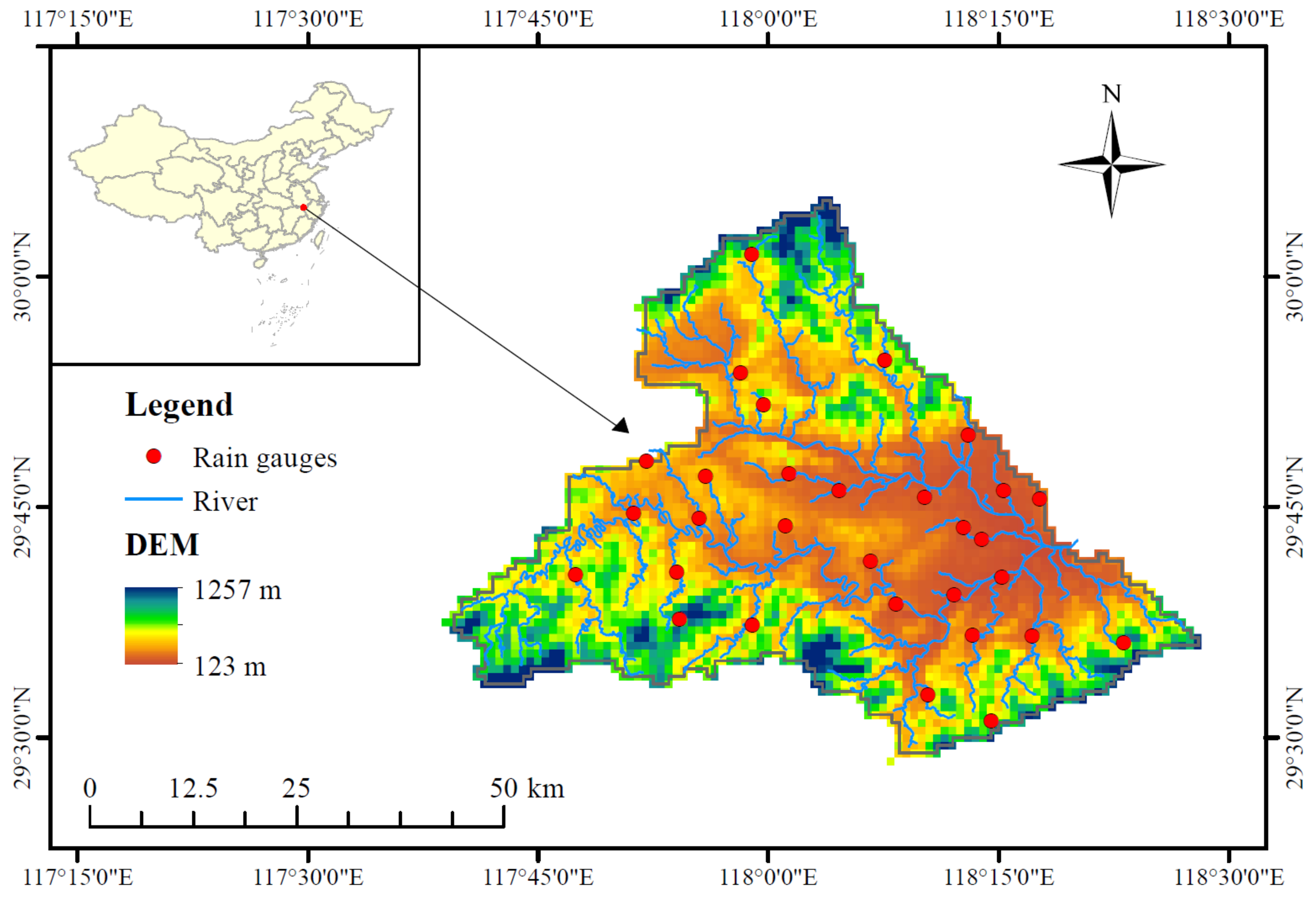
2.1. Study Area

Tunxi Watershed is located in Huangshan City, southeastern China. It is situated between 29.47°N–30.09°N and 117.65°E–118.47°E, and the total area is 2674 km2 (Figure 1). It is located in the transitional zone between the Jianghuai plain and the East China mountains and has typical north–south interlacing geographical features. The watershed is located in the subtropical monsoon humid climate zone, characterized by hot and humid summers and cool to mild winters [38,39,40]. The average annual precipitation is about 1800 mm, concentrated in May–September. It has the obvious characteristics of high precipitation and temperature in summer. The average annual temperature is approximately 17 °C. The dominant vegetation types in this region are evergreen broadleaf forest, evergreen needle-leaf trees, and bamboo [37,41,42]. The terrain in the middle of the basin is relatively flat, and the topographic conditions at the edges are complex. The elevation has an apparent spatial heterogeneity with the highest altitude of 1257 m and the lowest altitude of 123 m. The complex terrain, high intensity, and uneven spatiotemporal precipitation can easily lead to flash floods.

2.2. Data

2.2.1. Rain Gauge Data

Precipitation data covering 2018–2020 from 30 precipitation gauges in the Tunxi Watershed were selected as the reference data for evaluating the performance of the IMERG datasets. Precipitation was sampled every 5 min using tipping-bucket rain gauges with a 0.5 mm resolution. The 5 min precipitation was temporally aggregated to 30 min precipitation. The 30 precipitation gauges are evenly distributed across the Tunxi Watershed with a density of 0.011 set/km2. The precipitation data were provided by the Xin’anjiang Nested Experimental Watershed (http://hydro-lab.hhu.edu.cn/, accessed on 1 February 2023) [37].

2.2.2. IMERG Dataset

The Integrated Multi-satellite Retrievals for GPM (IMERG) algorithm fuses information from several satellite-based microwave and infrared precipitation estimates. The IMERG system is run three times, namely, early (~4 h), late (~14 h), and final (~3.5 months) runs (hereafter IMERG-E, IMERG-L, and IMERG-F). IMERG-F includes additional satellite data and was merged with monthly gauge information. Several data fields are included in each IMERG dataset showing how the estimates were computed to provide data quality information The HQprecipitation fields represent the merged microwave-only precipitation estimate and can identify the microwave satellite source from the HQprecipSource fields. IRprecipitation is IR-only precipitation estimate and can identify the weight of IR-only precipitation relative to the morphed merged microwave-only precipitation by IRkalmanFilterWeight. The IRkalmanFilterWeight values range from 0 to 100, where 0 is morph only, 100 is entirely based on IR, and anything in between is IR + morph. The IMERG-F precipitationUncal fields are recorded in the original multi-satellite-only half-hourly data. The IMERG-F precipitationcal fields are recorded precipitation data after gauge correction [43].
Global Precipitation Measurement Mission Integrated Multi-satellite Final Run V6B (hereafter, IMERG-F V6B) [43,44], which has been released as the latest version, is used to perform the data quality analysis. The IMERG-F V6B precipitationUncal dataset without monthly gauge adjustment is compared against the rain gauge. The IMERG-F precipitationUncal provides precipitation data with 30 min and 0.1 × 0.1 degree resolutions at global scale. We chose an overlapping time span from 2018 to 2020 as our study period. The bilinear interpolation method was used to downscale coarser satellite precipitation data to a fine spatial resolution (1 km). The input source includes five types of passive microwave (PMW) instruments (Table 1) and infrared (IR) observations.

3. Methodology

3.1. Evaluation of Detection Capability

The detection capability of IMERG was evaluated against gauge observation using a point-to-pixel method. Several statistical indexes were adopted to evaluate the performance of IMERG [25,27,45,46,47]. The threshold to distinguish rain/no rain events was set to 0.5 mm based on the resolution of the rain gauge. Hit events (H) represent the precipitation events detected by IMERG and gauge. False events (F) represent the precipitation events detected by IMERG but not observed by the gauge. Miss events (M) represent the precipitation events not detected by IMERG but observed by the gauge. Nonevents events (N) represent the precipitation events not detected by both IMERG and gauge. The probability of detection (POD), false alarm ratio (FAR), and critical success index (CSI) were used to evaluate the precipitation detection capability (Table 2). The Brier score (BS) is a function to measure the accuracy of probabilistic predictions [48]. A model with good performance has a score of 0, while the worst has a score of 1. All these statistical indexes can calculate the occurrence and nonoccurrence of precipitation events between IMERG and precipitation gauge data.

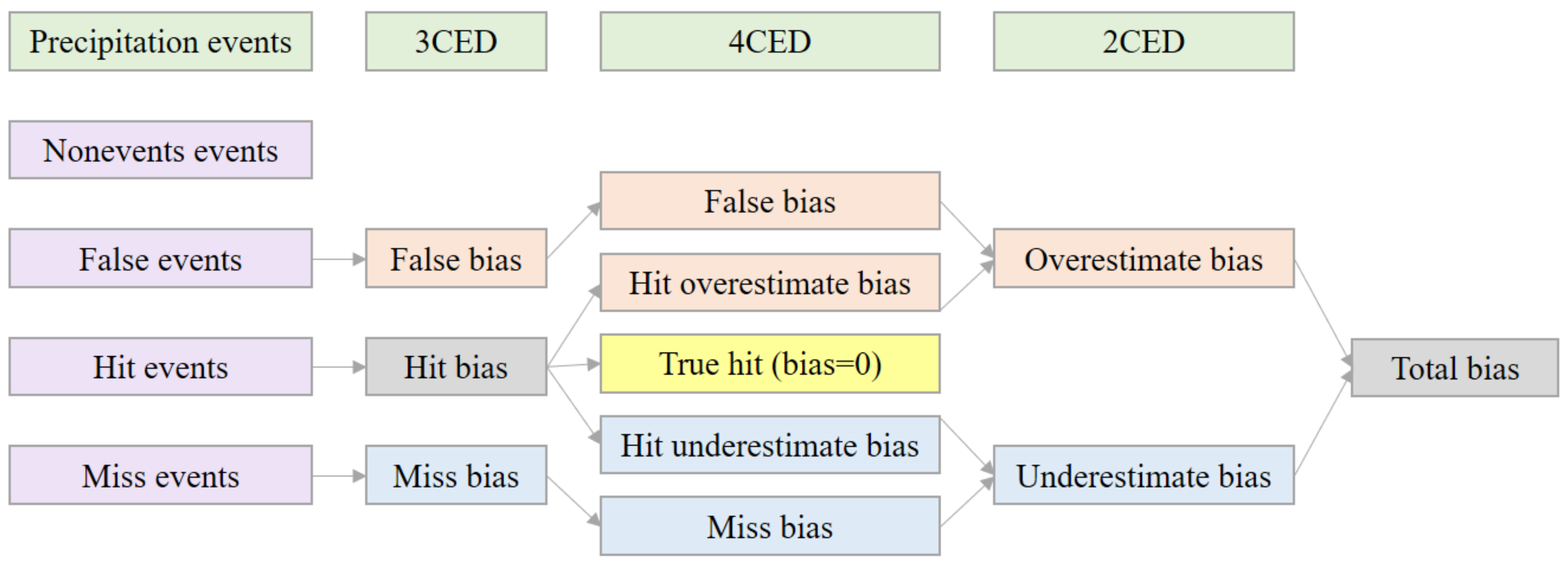
3.2. Four-Component Error Decomposition Method

In order to better quantify and trace the error sources of IMERG, based on the detection capability and estimation capacity, the total bias (TB) can be decomposed into several independent error components. Here, we used the 4CED to perform the IMERG data quality analysis. The traditional error decomposition method (hereafter called the three-component error decomposition method, 3CED) proposed by Tian et al. [20] decomposes the TB into three components, namely, hit bias (HB), false bias (FB), and miss bias (MB) (Table 3). Among the three independent error components, FB is always positive, and MB is always negative, while HB can be either positive or negative. Furthermore, the HB is further decomposed into the hit overestimate bias (HOB), hit underestimate bias (HUB), and true hit (bias = 0). Therefore, the 4CED includes HOB, HUB, FB, and MB [21,22]. The detailed mathematical formulas are listed in Table 3. HOB and FB are always positive among the four error components, while HUB and MB are always negative. Therefore, the TB can be decomposed into the overestimate bias (OB) and the underestimate bias (UB) using the two-component error decomposition method (2CED). OB is calculated as the sum of HOB and FB, and UB is calculated as the sum of HUB and MB. Moreover, the relationships between TN, OB, UB, HOB, HUB, FB, and MB is TB = OB + UB = (HOB + FB) + (HUB + MB) = HB + FB + MB (Figure 2).

3.3. Systematic and Random Error Decomposition

IMERG data derived from the retrieval results of multiple satellite sensors has its characteristics. Systematic error and random error decomposition can be used to perform error tracing. Systematic errors can reflect the characteristics of sensors and precipitation retrieval algorithms, while random errors are ubiquitous and unavoidable in observations. The mean square error was decomposed into systematic and random components as follows [4,24,49]:
i = 1 n ( S G ) 2 = i = 1 n ( S ^ G ) 2 + i = 1 n ( S S ^ ) 2
E S = i = 1 n ( S ^ G ) 2 i = 1 n ( S G ) 2 × 100 %
E R = i = 1 n ( S S ^ ) 2 i = 1 n ( S G ) 2 × 100 %
S ^ = a × G + b
where S ^ represents the precipitation, which is calculated by the additive error model. E S is the systematic error ratio, and E G is the random error ratio. a and b are the slope and intercept of the additive error model, respectively.

4. Results

4.1. General Analysis

The precipitation derived from the IMERG product was extracted over the Tunxi Watershed and compared with the gauge observations. The average annual precipitation at points or grids for gauge observation and IMERG were 1874 and 1676 mm, respectively. A preliminary comparison of IMERG with the reference data is shown in Figure 3. In general, IMERG is more consistent with the reference for Tunxi Watershed, except for a slight underestimation over mountain area. Figure 3a, the bias between the IMERG and gauge observation shows that IMERG tends to slightly underestimate the precipitation (bias < −200 mm) in mountainous terrain areas. The precipitation detected by IMERG at the elevation between 135 m and 369 m is close to the gauge measurements (−200 mm < bias < 200 mm). Elevation significantly influenced the accuracy of IMERG, and the accuracy of IMERG decreased with the increase of elevation. The relative bias is within 20% at 93.33% of the gauges in the Tunxi Watershed (Figure 3b). The correlation coefficient on the 30 min time scale ranges from 0.39 to 0.52 (Figure 3c), demonstrating a relatively poor performance on the data consistency, which is consistent with previous studies [13,46,50]. IMERG has closer annual precipitation with a poor correlation coefficient on the 30 min time scale, indicating that the detectability performance may cause a larger impact on the data quality on the 30 min time scale.

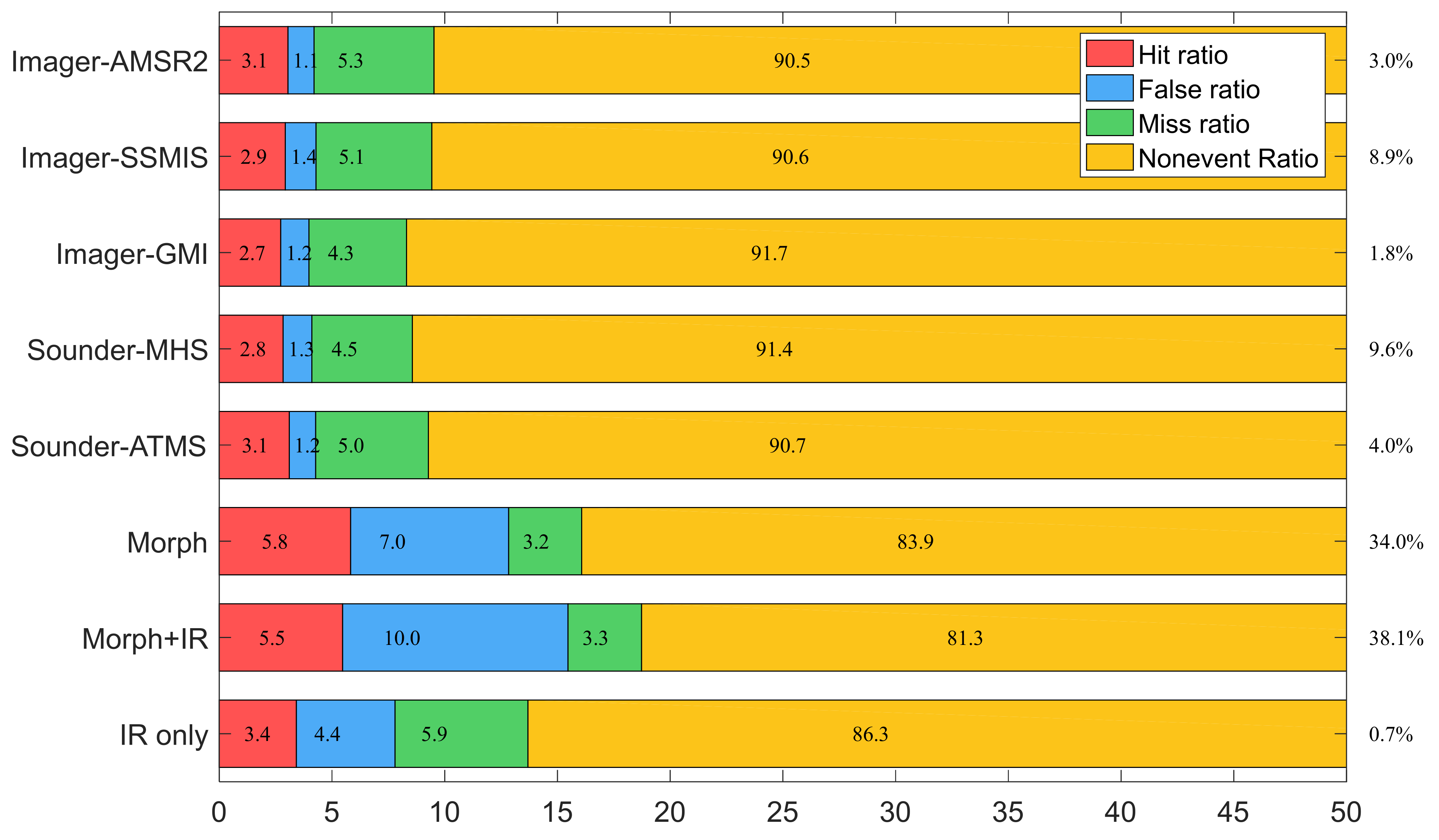
4.2. Detectability Performance

It is critical to analyze and trace the error contribution of IMERG and identify the input source (sensor type) and its features. Figure 4 shows the sample ratio and four types of precipitation events for all input sensor sources. Clearly, the sample ratio for IR (Morph, IR + Morph, and IR only) sources is 72.8%, which is much higher than the sample ratio for PMW (AMSR2, SSMIS, GMI, MHS, and ATMS) sources (27.2%). The precipitation data from IR sensor accounts for a significant proportion in the IMERG data. It means the precipitation data quality from the IR sources plays an important role in IMERG. Obviously, PMW sources had low HR, FR, and high MR. On the other hand, IR has high HR, FR, corresponding to a low MR. It indicates that IR sources overestimate rain rate occurrences because of the high HR, FR, and low MR. In summary, it is worth noting that IR has a high rate sample, and its detection capability contributed much error to IMERG.
Figure 5 shows the results of POD, FAR, and CSI for each input source used in IMERG. The POD values for Morph and Morph + IR are higher than 60%, while all the PMW sources have values between 36.3% and 38.8%, with tiny differences. On the other hand, for FAR, all the IR sources are higher than 50%, which is much higher than PWM sensors (27.5–31.8%). It indicates that IR tends to estimate false rainfall events. The CSI for PMW (32.5%) is higher than IR (30.1%), showing that PMW sensors have a good ability to detect precipitation for all precipitation events.
The BS was used to further analyze the IMERG precipitation detection and its accuracy. Compared with the sounder passive microwave sensor, the imager passive microwave sensor has a higher BS, indicating that the imager’s precipitation detection accuracy is slightly lower (Figure 6). Among the individual data sources, GMI has the lowest BS, indicating the high rate of prediction accuracy and low proportion of misreported and underreported precipitation events. It is worth noting that Morph + IR has the highest BS and the lowest accuracy rate, mainly due to its high false positive rate. Since that Morph + IR contributes the most to IMERG precipitation, improving its accuracy is crucial for improving the overall accuracy of IMERG data. Based on the analysis in Figure 4, Figure 5 and Figure 6, we can conclude that the detection errors, including false events and miss events, are the main error source of IMERG. Moreover, it is worth noting that GMI has the highest precision among all the sensors. GMI instruments aboard the GPM Core Observatory are designed to provide key information for sensing light and solid precipitation.

4.3. Four-Component Error Decomposition Results

Figure 7 shows the total bias and the four error decomposed components for the eight input sources of IMERG. Generally, the TB for all sensors is negative, which means all the sensors underestimate precipitation. Morph has the biggest |TB| of 4.08%, Morph + IR has the highest FB and |HUB|. For all the PMW sensors, |MB| is an important component among the four components, which leads to negative TB. Bias is not only related to the data quality but also to data quantity. IR only has a little effect on the quality of IMERG data because of its small sample size, despite its poor detectability performance. Morph and Morph + IR have a significant sample size and a considerable TB due to their poor detectability performance, resulting in a large TB. Therefore, improving the detectability and precision of the Morph and Morph + IR is essential to reduce the HOB, |HUB|, FB, and |MB|. For the TB, the Morph + IR is smaller than Morph, while Morph + IR has larger |HUB|, FB, and |MB|. The performance of Morph + IR is still questionable since the magnitude of TB may be adjusted due to the cancellation of positive values (HOB and FB) and negative values (HUB and MB).

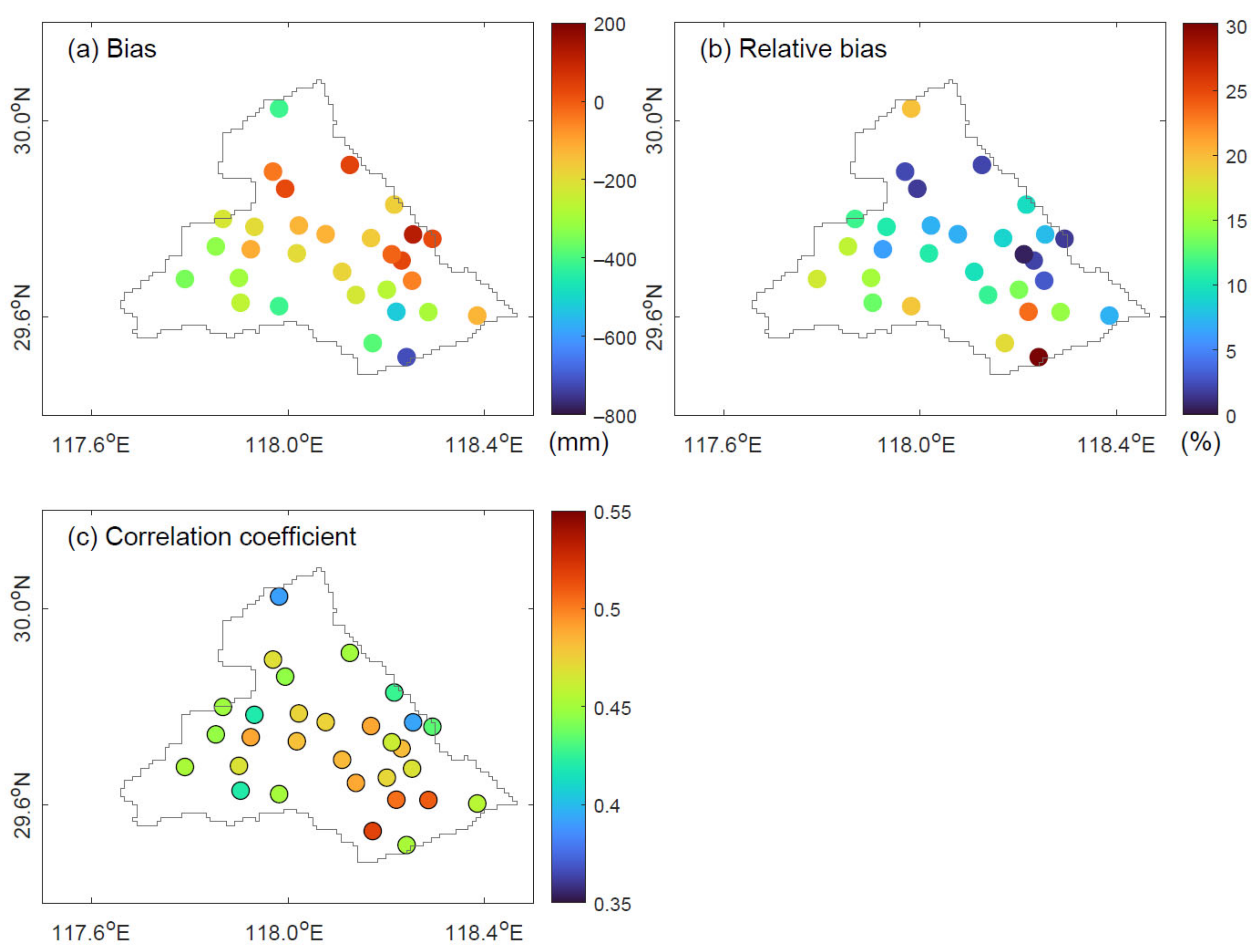
4.4. Systematic and Random Error Decomposition

The systematic and random error components of each sensor were estimated using an additive error model performed over Tunxi Watershed from 2018 to 2020. Figure 8 displays each sensor’s systematic and random components of total error. Clearly, all the PMW-sounder sensors exhibit a lower systematic error ratio (<27.94%), while PMW-imager sensors exhibit less random error (<39.0%). Systematic error is the prominent component for AMSR2, SSMIS, GMI, and Morph + IR. It should be noted that ATMS has the lowest systematic error of 7.8%, showing that most of the systematic error is removed.

5. Discussion

5.1. Error Decomposition

There are close connections between 2CED, 3CED, and 4CED (Section 3.2). 2CED and 3CED can be derived based on the 4CED. In Section 4.3, the 4CED has been used to identify the IMERG data error for each sensor. In addition, the relationships and differences between 2CED, 3CED, and 4CED are discussed.
Figure 9 depicts the three components of bias (HB, FB, and MB) for the eight input sources of IMERG. Compared to 4CED, 3CED has the same FB and MB as 4CED. Morph + IR has the biggest |HB| (9.26%) of all the sensors, followed by Morph (5.72%). For Morph + IR, the |HB|, HOB, and |HUB| are 9.26%, 6.12%, and 15.38%, respectively. The |HB|, HOB, and |HUB| for Morph are 5.723%, 8.10%, and 13.83%. Obviously, HB is underrepresented due to the cancelation of the positive HOB and the negative HUB. 4CED can describe the error component more comprehensively. For the PMW-sounder sensors, the HB is always positive.
Based on the 4CED method, TB can be further divided into OB and UB. OB is the sum of HOB and FB, while UB is the sum of HUB and MB. For all the sensors, |UB| is bigger than OB, suggesting that |UB| is the dominant factor of the error source (Figure 10). Additionally, Morph + IR has the biggest OB and |UB|, while the TB is smaller than Morph, indicating a cancellation effect of the overestimate and underestimate bias.

5.2. Error Source Analysis

The satellite precipitation estimate is retrieved from the PMW and IR sensors to meet the spatial and temporal requirements. The sampling frequency and precision from PMW and IR sensors are related to the accuracy of IMERG data. Figure 4, Figure 5, Figure 6 and Figure 7 show the sample ratio, detection ability, four-component error decomposition, and systematic and random error for each input source. In summary, PMW sensors (AMSR2, SSMIS, GMI, MHS, and ATMS) have the low sample ratio with high accuracy, while IR sensors (Morph, Morph + IR, IR only) have the high sample ratio with low accuracy.
IMERG is designed to inter-calibrate, merge, and interpolate satellite microwave precipitation estimates together with microwave-calibrated infrared (IR) satellite estimates. The sample ratio for PMW sensors is 27.2%. To compensate for the limited available sampling, microwave-calibrated IR satellite estimates are used when the PMW samples are too sparse. Therefore, it is important to launch more leo-satellites to obtain more PMW information for precipitation estimates.
The frequent sampling and poor detection ability result in significant error in IMERG data. Therefore, it is essential to improve the detectability of IR sensors. The indirect relationship between IR brightness temperature and precipitation is used to calculate the precipitation. For PERSIANN-CSS, the 60°N-S latitude belt is divided into 24 sub-regions to perform regional training and parallel processing [51]. Chen et al. [52] found that the input source error of GPM-GSMaP is impacted by geographic and climatic factors. For the improvement of IMERG, more sub-regions related to latitude, topography, climatic, and other factors should be considered to get more accurate indirect relationship between IR brightness temperature and precipitation. In addition, the three temperature levels (220 K, 235 K, and 253 K) are used to extract cloud features at different altitudes. More temperature levels can be divided to perform precipitation calculations at different altitudes and regions. Recently, intelligent algorithms have demonstrated good predictive capability in many fields [53,54,55,56,57,58]. The development of intelligent algorithms provides new insight into precipitation prediction based on IR sensor.

5.3. Uncertainty of Gauge Observation

The evaluation of satellite precipitation estimates depends on surface gauge observations. When using rain gauge measurements as a benchmark, considering their density is important [8]. In the Tunxi Watershed, there is a typical catchment of 0.55 km2, and 13 precipitation stations are evenly distributed in the typical catchment at different elevations, slopes, and aspects. The method of measuring precipitation in the typical catchment is the same as in the Tunxi Watershed, using the same rain gauge and recording the data every 5 min. The annual precipitationfor the 13 precipitation stations are 2214, 2172, 2303, 2206, 2180, 2231, 2126, 2137, 1882, 1685, 2268, 2157, and 2289 mm, respectively. The coefficient of variation (Cv) for annual precipitation is 0.0809, with the mean, maximum, and minimum values of 2142, 2303, and 1685 mm, respectively. The observations show that the precipitation has small spatial heterogeneity in the typical catchment. In addition, it has been demonstrated by previous research that the spatial variability of precipitation across the Tunxi Watershed follows simple scaling and increases as the drainage area increases, leading to larger spatial heterogeneity [37]. The annual precipitation in the Tunxi watershed is 1874 mm, and the corresponding Cv is 0.1122. The annual precipitation and Cv of typical catchment and Tunxi Watershed are very close. Therefore, the rain gauge can capture the spatial pattern of the Tunxi Watershed, indicating that the rain gauge density can reach the requirement for the satellite evaluation.

6. Conclusions

In this study, the 4CED and systematic and random error decomposition are used to quantify and trace the error characteristics of the eight input sources used in the IMERG dataset. The evaluation of IMERG data includes detectability performance, 4CED, and systematic and random errors. The primary conclusions are as follows.
(1)
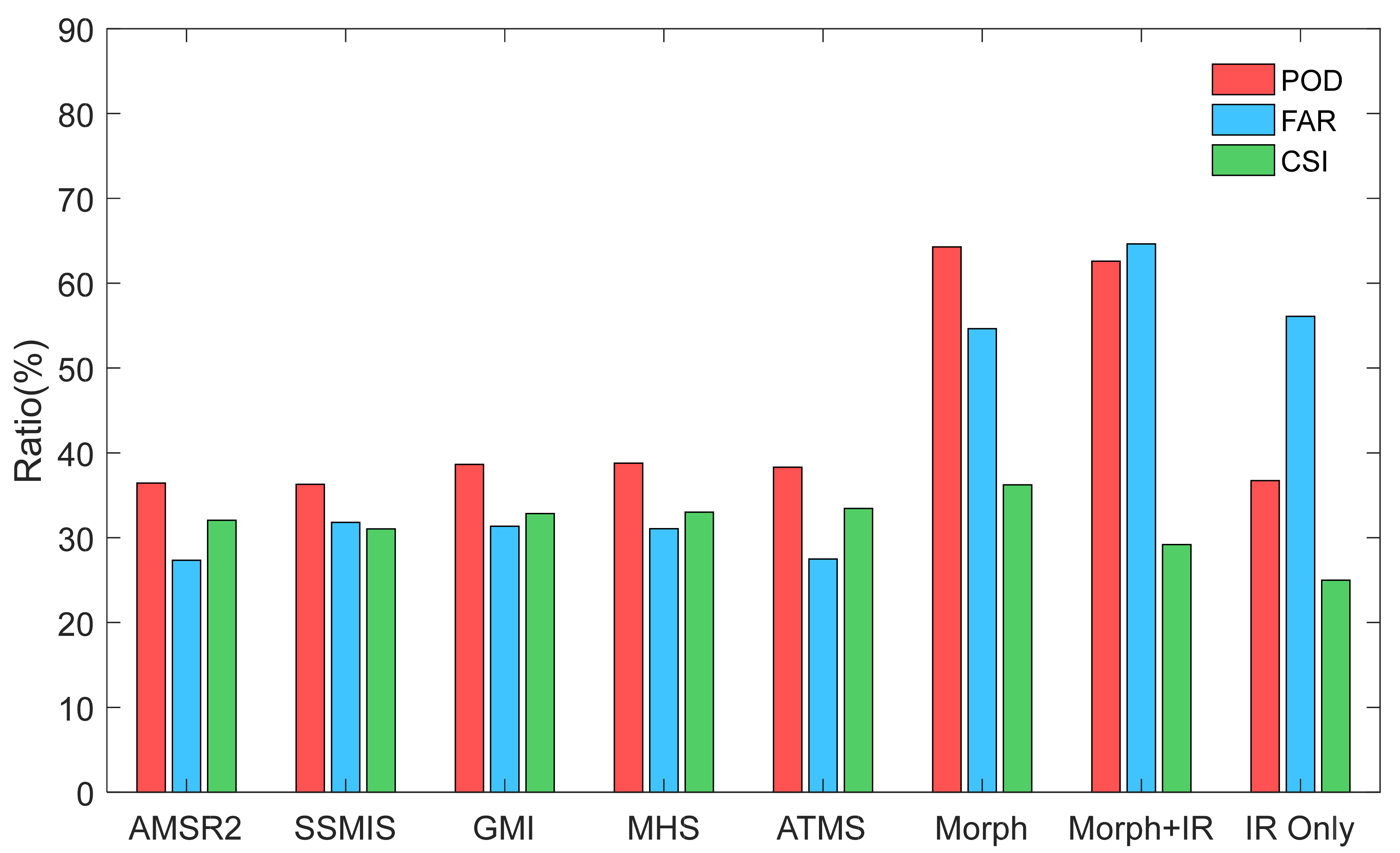
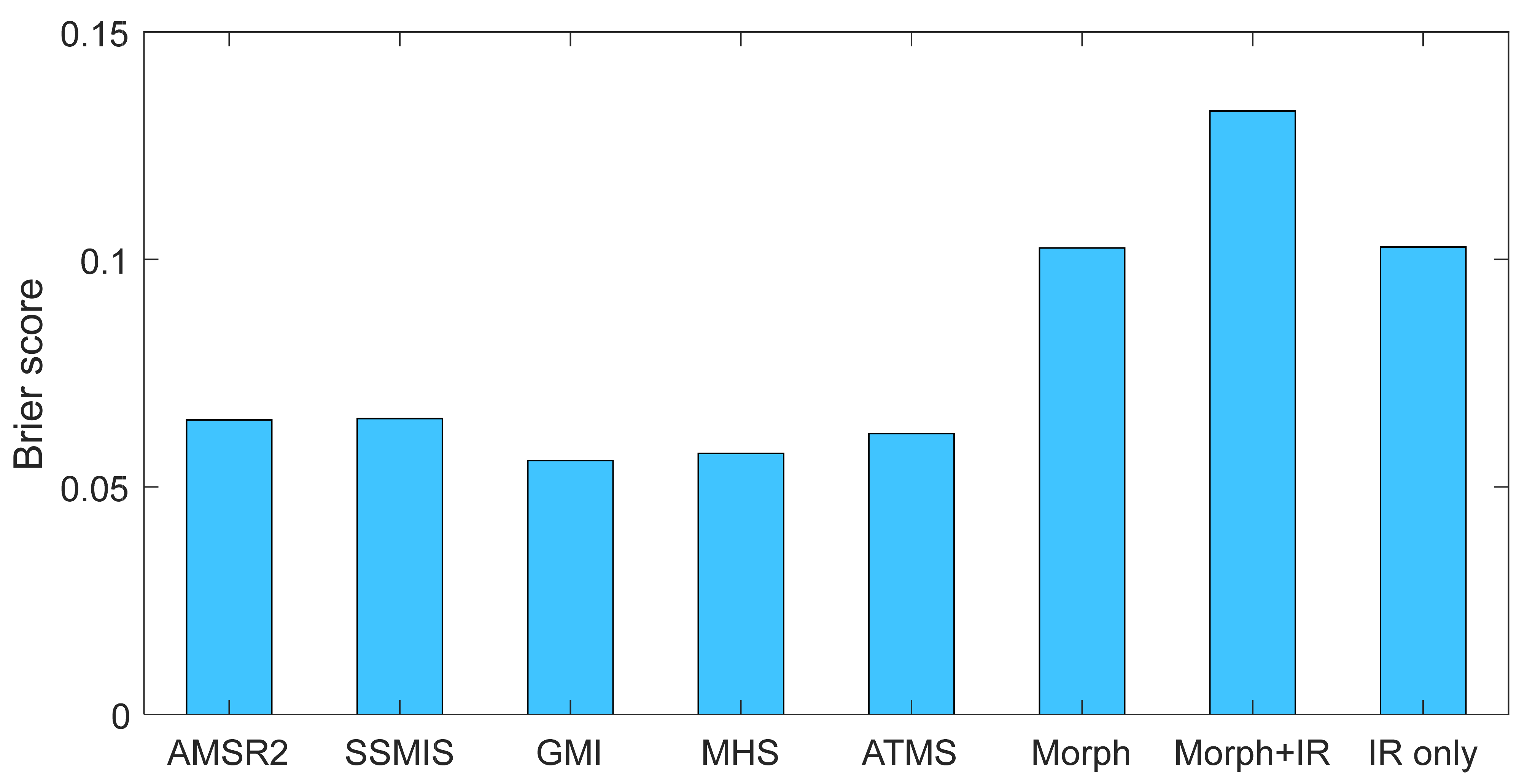
For detectability, the sample ratio for IR (Morph, IR + Morph, and IR only) is much higher than for PMW (AMSR2, SSMIS, GMI, MHS, and ATMS). The IR sensor has a high HR, FR, POD, and FAR, indicating that IR is sensitive to light precipitation events and tends to predict a false signal for the satellite estimate. The poor performance of CSI and BS for IR sensors is mainly due to the high false ratio.
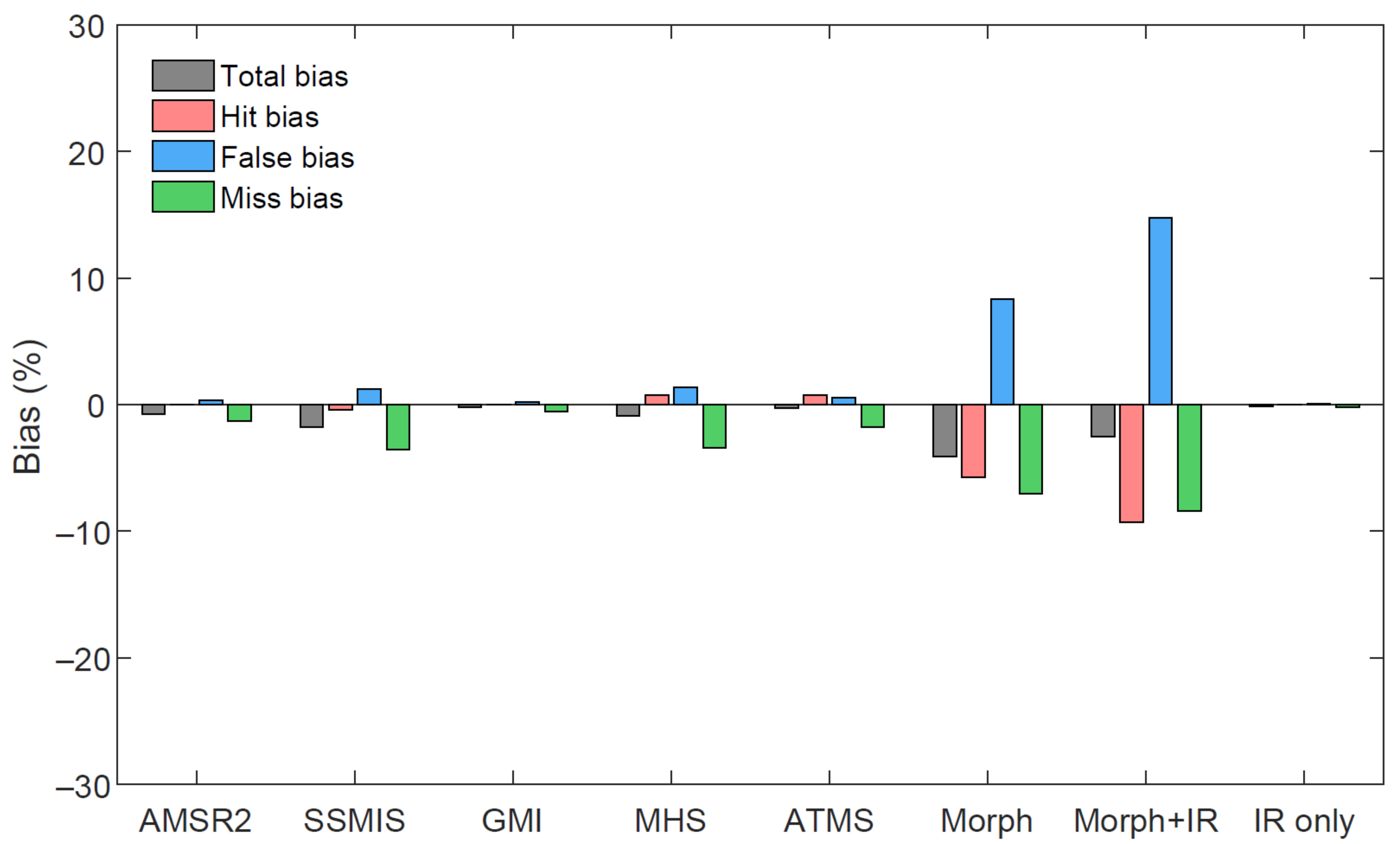
(2)
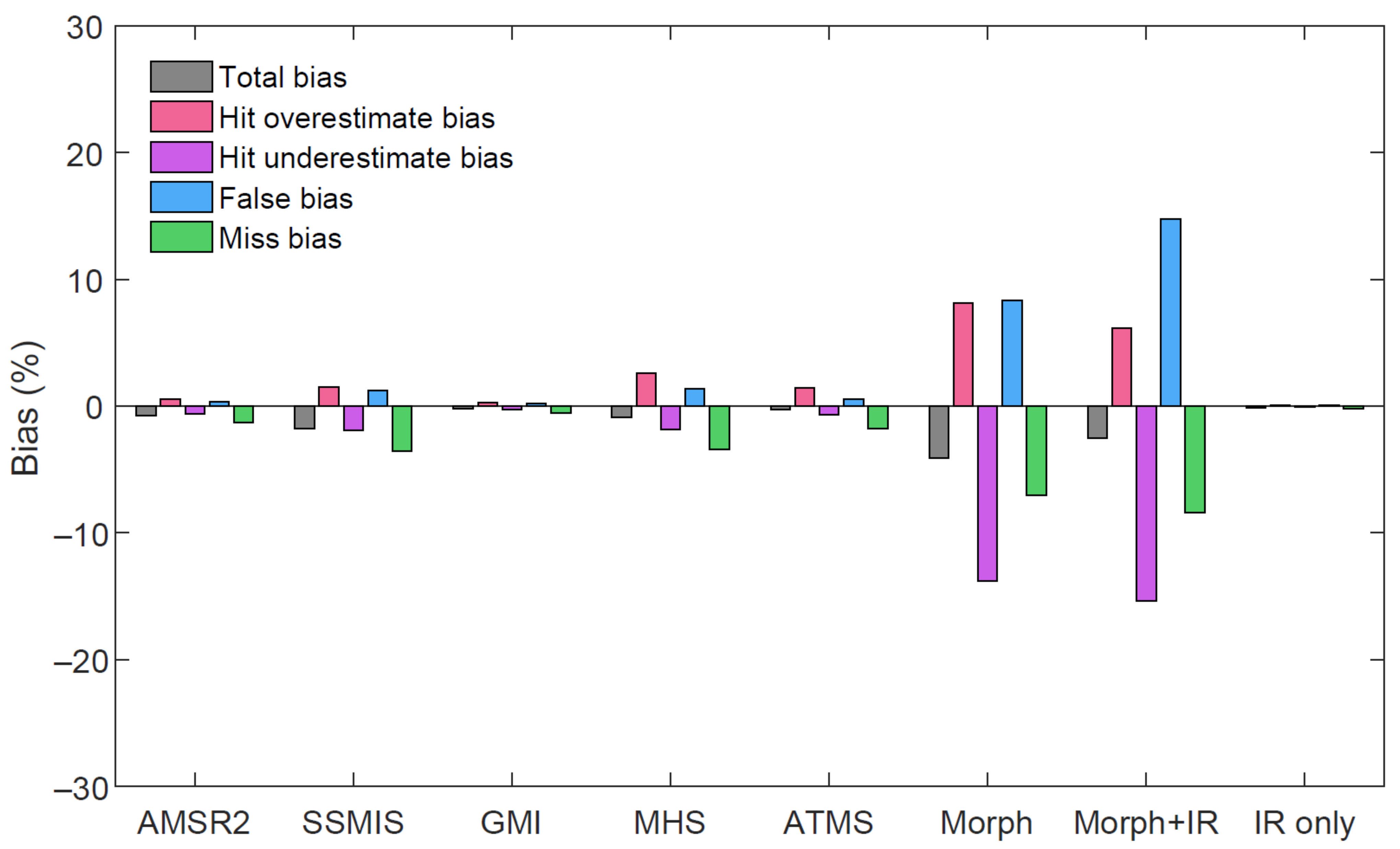
Based on the 4CED, the TB can be decomposed into HOB, HUB, FB, and MB. HOB and FB are always positive among the four error components, while HUB and MB are always negative. The magnitude of HOB and |HUB| is higher than |HB| because of the unavoidable cancellation during the HB calculations process. Generally, the TB for all sensors is negative, meaning that all the sensors underestimate precipitation. Morph and Morph + IR have considerable bias related to the prediction ability and the sample size. It is crucial to reduce the FR to improve the detectability of IR sensors due to their high sample size.
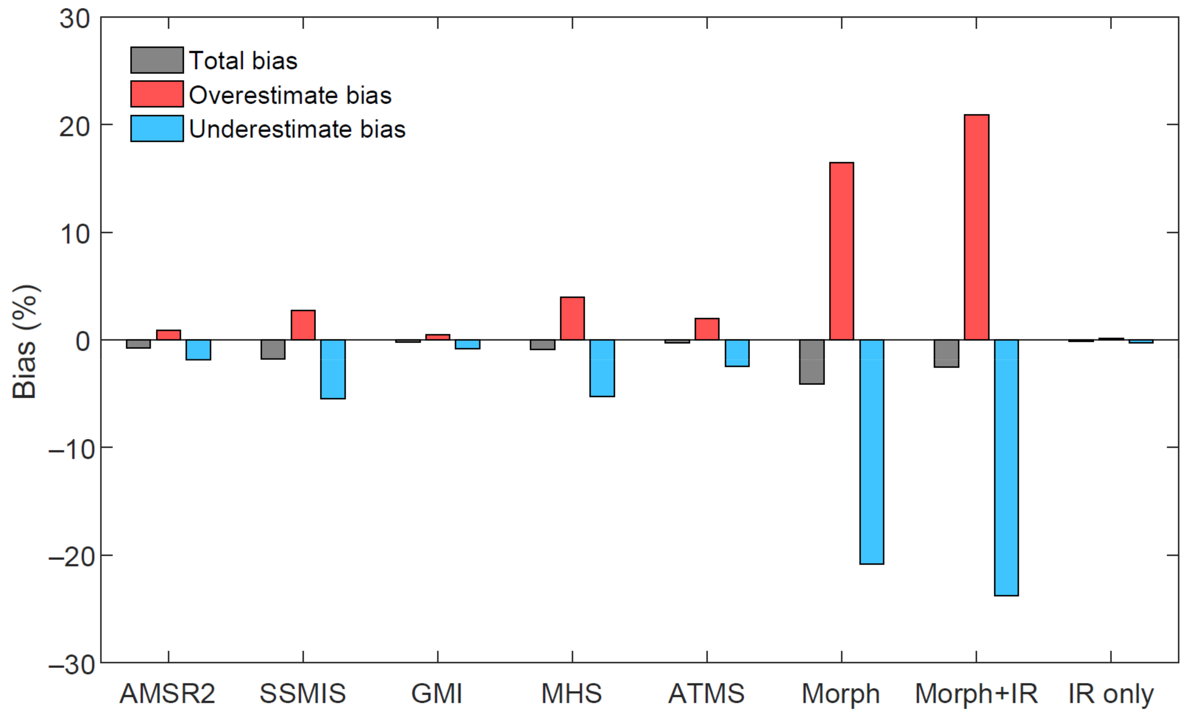
(3)
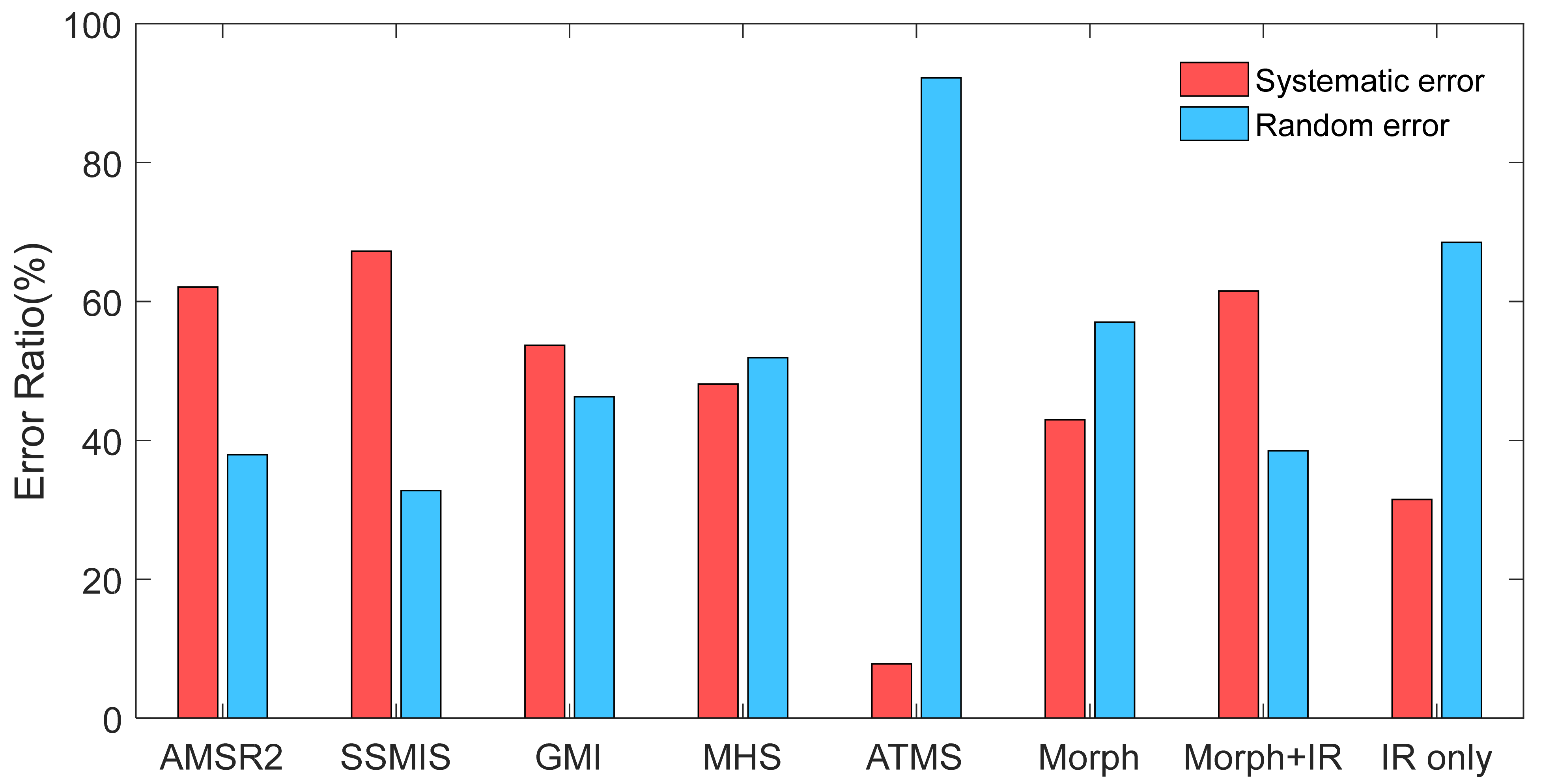
The systematic and random error components were assessed using the additive error model. Systematic error is the prominent component for AMSR2, SSMIS, GMI, and Morph + IR, indicating that the retrieval algorithm for these sensors needs further improvement.

Author Contributions

Conceptualization, Y.L., K.Z. and A.B.; Methodology, Y.L., K.Z. and A.B.; Validation, X.S.; Writing–original draft, Y.L.; Writing–review & editing, K.Z., A.B., X.S. and Y.C.; Visualization, Y.L. and Y.C.; Supervision, K.Z.; Funding acquisition, K.Z. All authors have read and agreed to the published version of the manuscript.

Funding

This research was funded by National Natural Science Foundation of China, grant number 51879067; Fundamental Research Funds for the Central Universities, grant number B200204038; Hydraulic Science and Technology Plan Foundation of Shaanxi Province, grant number 2019slkj-B1.

Data Availability Statement

IMERG dataset: https://disc.gsfc.nasa.gov/, accessed on 1 February 2023.

Conflicts of Interest

The authors declare no conflict of interest.

References

  1. Sun, Q.; Miao, C.; Duan, Q.; Ashouri, H.; Sorooshian, S.; Hsu, K.L. A review of global precipitation data sets: Data sources, estimation, and intercomparisons. Rev. Geophys. 2018, 56, 79–107. [Google Scholar] [CrossRef] [Green Version]
  2. Tang, G.; Ma, Y.; Long, D.; Zhong, L.; Hong, Y. Evaluation of GPM Day-1 IMERG and TMPA Version-7 legacy products over Mainland China at multiple spatiotemporal scales. J. Hydrol. 2016, 533, 152–167. [Google Scholar] [CrossRef]
  3. Kidd, C.; Huffman, G. Global precipitation measurement. Meteorol. Appl. 2011, 18, 334–353. [Google Scholar] [CrossRef]
  4. Lei, H.; Zhao, H.; Ao, T. Ground validation and error decomposition for six state-of-the-art satellite precipitation products over mainland China. Atmos. Res. 2022, 269, 106017. [Google Scholar] [CrossRef]
  5. Liu, C.-Y.; Aryastana, P.; Liu, G.-R.; Huang, W.-R. Assessment of satellite precipitation product estimates over Bali Island. Atmos. Res. 2020, 244, 105032. [Google Scholar] [CrossRef]
  6. Derin, Y.; Kirstetter, P.-E.; Gourley, J.J. Evaluation of IMERG Satellite Precipitation over the Land–Coast–Ocean Continuum. Part I: Detection. J. Hydrometeorol. 2021, 22, 2843–2859. [Google Scholar] [CrossRef]
  7. Kirstetter, P.E.; Karbalaee, N.; Hsu, K.; Hong, Y. Probabilistic precipitation rate estimates with space-based infrared sensors. Q. J. R. Meteorol. Soc. 2018, 144, 191–205. [Google Scholar] [CrossRef] [Green Version]
  8. Maggioni, V.; Massari, C. On the performance of satellite precipitation products in riverine flood modeling: A review. J. Hydrol. 2018, 558, 214–224. [Google Scholar] [CrossRef]
  9. Huffman, G.J.; Bolvin, D.T.; Nelkin, E.J.; Wolff, D.B.; Adler, R.F.; Gu, G.; Hong, Y.; Bowman, K.P.; Stocker, E.F. The TRMM Multisatellite Precipitation Analysis (TMPA): Quasi-Global, Multiyear, Combined-Sensor Precipitation Estimates at Fine Scales. J. Hydrometeorol. 2007, 8, 38–55. [Google Scholar] [CrossRef]
  10. Maggioni, V.; Meyers, P.C.; Robinson, M.D. A Review of Merged High-Resolution Satellite Precipitation Product Accuracy during the Tropical Rainfall Measuring Mission (TRMM) Era. J. Hydrometeorol. 2016, 17, 1101–1117. [Google Scholar] [CrossRef]
  11. Pradhan, R.K.; Markonis, Y.; Vargas Godoy, M.R.; Villalba-Pradas, A.; Andreadis, K.M.; Nikolopoulos, E.I.; Papalexiou, S.M.; Rahim, A.; Tapiador, F.J.; Hanel, M. Review of GPM IMERG performance: A global perspective. Remote Sens. Environ. 2022, 268, 112754. [Google Scholar] [CrossRef]
  12. Sapiano, M.; Arkin, P. An intercomparison and validation of high-resolution satellite precipitation estimates with 3-hourly gauge data. J. Hydrometeorol. 2009, 10, 149–166. [Google Scholar] [CrossRef]
  13. Ayat, H.; Evans, J.P.; Behrangi, A. How do different sensors impact IMERG precipitation estimates during hurricane days? Remote Sens. Environ. 2021, 259, 112417. [Google Scholar] [CrossRef]
  14. Zhu, Z.; Yong, B.; Ke, L.; Wang, G.; Ren, L.; Chen, X. Tracing the error sources of global satellite mapping of precipitation for GPM (GPM-GSMaP) over the Tibetan Plateau, China. IEEE J. Sel. Top. Appl. Earth Obs. Remote Sens. 2018, 11, 2181–2191. [Google Scholar] [CrossRef]
  15. Hsu, K.-l.; Gao, X.; Sorooshian, S.; Gupta, H.V. Precipitation estimation from remotely sensed information using artificial neural networks. J. Appl. Meteorol. 1997, 36, 1176–1190. [Google Scholar] [CrossRef]
  16. Joyce, R.J.; Janowiak, J.E.; Arkin, P.A.; Xie, P. CMORPH: A method that produces global precipitation estimates from passive microwave and infrared data at high spatial and temporal resolution. J. Hydrometeorol. 2004, 5, 487–503. [Google Scholar] [CrossRef]
  17. Ushio, T.; Sasashige, K.; Kubota, T.; Shige, S.; Okamoto, K.i.; Aonashi, K.; Inoue, T.; Takahashi, N.; Iguchi, T.; Kachi, M. A Kalman filter approach to the Global Satellite Mapping of Precipitation (GSMaP) from combined passive microwave and infrared radiometric data. J. Meteorol. Soc. Japan. Ser. II 2009, 87, 137–151. [Google Scholar] [CrossRef] [Green Version]
  18. Sorooshian, S.; Hsu, K.-L.; Gao, X.; Gupta, H.V.; Imam, B.; Braithwaite, D. Evaluation of PERSIANN system satellite-based estimates of tropical rainfall. Bull. Am. Meteorol. Soc. 2000, 81, 2035–2046. [Google Scholar] [CrossRef]
  19. Alijanian, M.; Rakhshandehroo, G.R.; Mishra, A.; Dehghani, M. Evaluation of remotely sensed precipitation estimates using PERSIANN-CDR and MSWEP for spatio-temporal drought assessment over Iran. J. Hydrol. 2019, 579, 124189. [Google Scholar] [CrossRef]
  20. Tian, Y.; Peters-Lidard, C.D.; Eylander, J.B.; Joyce, R.J.; Huffman, G.J.; Adler, R.F.; Hsu, K.l.; Turk, F.J.; Garcia, M.; Zeng, J. Component analysis of errors in satellite-based precipitation estimates. J. Geophys. Res. Atmos. 2009, 114, D24101. [Google Scholar] [CrossRef] [Green Version]
  21. Chaudhary, S.; Dhanya, C.T. An improved error decomposition scheme for satellite-based precipitation products. J. Hydrol. 2021, 598, 126434. [Google Scholar] [CrossRef]
  22. Zhang, Y.; Ye, A.; Nguyen, P.; Analui, B.; Sorooshian, S.; Hsu, K. New insights into error decomposition for precipitation products. Geophys. Res. Lett. 2021, 48, e2021GL094092. [Google Scholar] [CrossRef]
  23. Ma, Y.Z.; Hong, Y.; Chen, Y.; Yang, Y.; Tang, G.Q.; Yao, Y.J.; Long, D.; Li, C.M.; Han, Z.Y.; Liu, R.H. Performance of Optimally Merged Multisatellite Precipitation Products Using the Dynamic Bayesian Model Averaging Scheme over the Tibetan Plateau. J. Geophys. Res.-Atmos. 2018, 123, 814–834. [Google Scholar] [CrossRef] [Green Version]
  24. AghaKouchak, A.; Mehran, A.; Norouzi, H.; Behrangi, A. Systematic and random error components in satellite precipitation data sets. Geophys. Res. Lett. 2012, 39, L09406. [Google Scholar] [CrossRef] [Green Version]
  25. Maggioni, V.; Sapiano, M.R.; Adler, R.F. Estimating uncertainties in high-resolution satellite precipitation products: Systematic or random error? J. Hydrometeorol. 2016, 17, 1119–1129. [Google Scholar] [CrossRef]
  26. Derin, Y.; Anagnostou, E.; Anagnostou, M.N.; Kalogiros, J.; Casella, D.; Marra, A.C.; Panegrossi, G.; Sanò, P. Passive microwave rainfall error analysis using high-resolution X-band dual-polarization radar observations in complex terrain. IEEE Trans. Geosci. Remote Sens. 2018, 56, 2565–2586. [Google Scholar] [CrossRef]
  27. Gebregiorgis, A.S.; Kirstetter, P.E.; Hong, Y.E.; Gourley, J.J.; Huffman, G.J.; Petersen, W.A.; Xue, X.; Schwaller, M.R. To what extent is the day 1 GPM IMERG satellite precipitation estimate improved as compared to TRMM TMPA-RT? J. Geophys. Res. Atmos. 2018, 123, 1694–1707. [Google Scholar] [CrossRef]
  28. Guilloteau, C.; Foufoula-Georgiou, E.; Kummerow, C.D. Global multiscale evaluation of satellite passive microwave retrieval of precipitation during the TRMM and GPM eras: Effective resolution and regional diagnostics for future algorithm development. J. Hydrometeorol. 2017, 18, 3051–3070. [Google Scholar] [CrossRef]
  29. Tan, J.; Petersen, W.A.; Tokay, A. A novel approach to identify sources of errors in IMERG for GPM ground validation. J. Hydrometeorol. 2016, 17, 2477–2491. [Google Scholar] [CrossRef]
  30. Zhu, Y.; Wang, H.; Zhou, W.; Ma, J. Recent changes in the summer precipitation pattern in East China and the background circulation. Clim. Dyn. 2011, 36, 1463–1473. [Google Scholar] [CrossRef]
  31. Chao, L.J.; Zhang, K.; Li, Z.J.; Wang, J.F.; Yao, C.; Li, Q.L. Applicability assessment of the CASCade Two Dimensional SEDiment (CASC2D-SED) distributed hydrological model for flood forecasting across four typical medium and small watersheds in China. J. Flood Risk Manag. 2019, 12, e12518. [Google Scholar] [CrossRef] [Green Version]
  32. Yao, C.; Li, Z.; Yu, Z.; Zhang, K. A priori parameter estimates for a distributed, grid-based Xinanjiang model using geographically based information. J. Hydrol. 2012, 468–469, 47–62. [Google Scholar] [CrossRef]
  33. Zang, S.; Li, Z.; Zhang, K.; Yao, C.; Liu, Z.; Wang, J.; Huang, Y.; Wang, S. Improving the flood prediction capability of the Xin’anjiang model by formulating a new physics-based routing framework and a key routing parameter estimation method. J. Hydrol. 2021, 603, 126867. [Google Scholar] [CrossRef]
  34. Wu, C.; Huang, G.; Yu, H.; Chen, Z.; Ma, J. Impact of Climate Change on Reservoir Flood Control in the Upstream Area of the Beijiang River Basin, South China. J. Hydrometeorol. 2014, 15, 2203–2218. [Google Scholar] [CrossRef]
  35. Xu, Y.; Huang, X.; Zhang, Y.; Lin, W.; Lin, E. Statistical Analyses of Climate Change Scenarios over China in the 21st Century. Adv. Clim. Chang. Res. 2006, 2, 50–53. [Google Scholar]
  36. Fu, G.; Yu, J.; Yu, X.; Ouyang, R.; Min, L. Temporal variation of extreme rainfall events in China, 1961–2009. J. Hydrol. 2013, 487, 48–59. [Google Scholar] [CrossRef]
  37. Zhang, K.; Li, Y.; Yu, Z.; Yang, T.; Xu, J.; Chao, L.; Ni, J.; Wang, L.; Gao, Y.; Hu, Y.; et al. Xin’anjiang Nested Experimental Watershed (XAJ-NEW) for Understanding Multiscale Water Cycle: Scientific Objectives and Experimental Design. Engineering 2022, 18, 207–217. [Google Scholar] [CrossRef]
  38. Li, Z.; Liu, M.; Zhao, Y.; Liang, T.; Sha, J.; Wang, Y. Application of Regional Nutrient Management Model in Tunxi Catchment: In Support of the Trans-boundary Eco-compensation in Eastern China. Clean-Soil Air Water 2014, 42, 1729–1739. [Google Scholar] [CrossRef]
  39. Qi, Z.; Kang, G.; Chu, C.; Qiu, Y.; Xu, Z.; Wang, Y. Comparison of SWAT and GWLF Model Simulation Performance in Humid South and Semi-Arid North of China. Water 2017, 9, 567. [Google Scholar] [CrossRef] [Green Version]
  40. Zhao, J.; Xu, J.; Cheng, L.; Jin, J.; Li, X.; Chen, N.; Han, D.; Zhong, Y. The evolvement mechanism of hydro-meteorological elements under climate change and the interaction impacts in Xin’anjiang Basin, China. Stoch. Environ. Res. Risk Assess. 2019, 33, 1159–1173. [Google Scholar] [CrossRef]
  41. Yan, L.; Chen, C.; Hang, T.; Hu, Y. A stream prediction model based on attention-LSTM. Earth Sci. Inform. 2021, 14, 723–733. [Google Scholar] [CrossRef]
  42. Qi, Z.; Kang, G.; Shen, M.; Wang, Y.; Chu, C. The Improvement in GWLF Model Simulation Performance in Watershed Hydrology by Changing the Transport Framework. Water Resour. Manag. 2019, 33, 923–937. [Google Scholar] [CrossRef]
  43. Huffman, G.J.; Bolvin, D.T.; Braithwaite, D.; Hsu, K.; Joyce, R.; Xie, P.; Yoo, S.-H. NASA global precipitation measurement (GPM) integrated multi-satellite retrievals for GPM (IMERG). Algorithm Theor. Basis Doc. (ATBD) Version 2015, 4, 26. [Google Scholar]
  44. Huffman, G.J. The Transition in Multi-Satellite Products from TRMM to GPM (TMPA to IMERG). Algorithm Information Document. 2019. Available online: https://docserver.gesdisc.eosdis.nasa.gov/public/project/GPM/TMPA-to-IMERG_transition.pdf (accessed on 2 November 2021).
  45. Moazami, S.; Najafi, M.R. A comprehensive evaluation of GPM-IMERG V06 and MRMS with hourly ground-based precipitation observations across Canada. J. Hydrol. 2021, 594, 125929. [Google Scholar] [CrossRef]
  46. Wang, S.; Liu, J.; Wang, J.; Qiao, X.; Zhang, J. Evaluation of GPM IMERG V05B and TRMM 3B42V7 Precipitation products over high mountainous tributaries in Lhasa with dense rain gauges. Remote Sens. 2019, 11, 2080. [Google Scholar] [CrossRef] [Green Version]
  47. Tang, S.; Li, R.; He, J.; Fan, X.; Wang, H.; Yao, S. Seasonal error component analysis of the GPM IMERG version 05 precipitation estimations over Sichuan basin of China. Earth Space Sci. 2021, 8, e2020EA001259. [Google Scholar] [CrossRef]
  48. Murphy, A.H. A New Vector Partition of the Probability Score. J. Appl. Meteorol. Climatol. 1973, 12, 595–600. [Google Scholar] [CrossRef]
  49. Chen, H.; Yong, B.; Kirstetter, P.-E.; Wang, L.; Hong, Y. Global component analysis of errors in three satellite-only global precipitation estimates. Hydrol. Earth Syst. Sci. 2021, 25, 3087–3104. [Google Scholar] [CrossRef]
  50. Yuan, F.; Wang, B.; Shi, C.; Cui, W.; Zhao, C.; Liu, Y.; Ren, L.; Zhang, L.; Zhu, Y.; Chen, T. Evaluation of hydrological utility of IMERG Final run V05 and TMPA 3B42V7 satellite precipitation products in the Yellow River source region, China. J. Hydrol. 2018, 567, 696–711. [Google Scholar] [CrossRef]
  51. Hong, Y.; Hsu, K.-L.; Sorooshian, S.; Gao, X. Precipitation Estimation from Remotely Sensed Imagery Using an Artificial Neural Network Cloud Classification System. J. Appl. Meteorol. 2004, 43, 1834–1853. [Google Scholar] [CrossRef] [Green Version]
  52. Chen, H.; Yong, B.; Gourley, J.J.; Liu, J.; Ren, L.; Wang, W.; Hong, Y.; Zhang, J. Impact of the crucial geographic and climatic factors on the input source errors of GPM-based global satellite precipitation estimates. J. Hydrol. 2019, 575, 1–16. [Google Scholar] [CrossRef]
  53. Ahmed, K.; Sachindra, D.; Shahid, S.; Iqbal, Z.; Nawaz, N.; Khan, N. Multi-model ensemble predictions of precipitation and temperature using machine learning algorithms. Atmos. Res. 2020, 236, 104806. [Google Scholar] [CrossRef]
  54. Ali, M.M.; Paul, B.K.; Ahmed, K.; Bui, F.M.; Quinn, J.M.; Moni, M.A. Heart disease prediction using supervised machine learning algorithms: Performance analysis and comparison. Comput. Biol. Med. 2021, 136, 104672. [Google Scholar] [CrossRef]
  55. Pandian, A.P. Performance evaluation and comparison using deep learning techniques in sentiment analysis. J. Soft Comput. Paradig. (JSCP) 2021, 3, 123–134. [Google Scholar]
  56. Saranya, T.; Sridevi, S.; Deisy, C.; Chung, T.D.; Khan, M.A. Performance analysis of machine learning algorithms in intrusion detection system: A review. Procedia Comput. Sci. 2020, 171, 1251–1260. [Google Scholar] [CrossRef]
  57. Schlef, K.E.; Moradkhani, H.; Lall, U. Atmospheric circulation patterns associated with extreme United States floods identified via machine learning. Sci. Rep. 2019, 9, 7171. [Google Scholar] [CrossRef] [Green Version]
  58. Tsakanikas, P.; Karnavas, A.; Panagou, E.Z.; Nychas, G.-J. A machine learning workflow for raw food spectroscopic classification in a future industry. Sci. Rep. 2020, 10, 11212. [Google Scholar] [CrossRef]
Figure 1. Location of the Tunxi Watershed and the distribution of rain gauges.
Remotesensing 15 01710 g001
Figure 2. The relationships between 3CED, 4CED, and 2CED.
Remotesensing 15 01710 g002
Figure 3. Spatial distribution of (a) bias and (b) relative bias of annual precipitation and (c) correlation coefficient between ground stations and IMERG (point-to-pixel) on 30 min time scale. The point with black circle means it has passed the significant test with the significance level of 0.05.
Remotesensing 15 01710 g003
Figure 4. Hit, miss, false, and nonevent ratios for each input source in IMERG. The values at the right indicate the sample ratio.
Remotesensing 15 01710 g004
Figure 5. The POD, FAR, and CSI for each input source used in IMERG.
Remotesensing 15 01710 g005
Figure 6. The Brier score for each input source used in IMERG.
Remotesensing 15 01710 g006
Figure 7. The total bias (TB), hit overestimate bias (HOB), hit underestimate bias (HUB), false bias (FB), and miss bias (MB) components for each input source used in IMERG over the Tunxi Watershed.
Remotesensing 15 01710 g007
Figure 8. The systematic and random error for each input source used in IMERG.
Remotesensing 15 01710 g008
Figure 9. The total bias (TB), hit bias (HB), false bias (FB), and miss bias (MB) components for each input source used in IMERG over the Tunxi watershed.
Remotesensing 15 01710 g009
Figure 10. The total bias (TB), overestimate bias (OB), and underestimate bias (UB) components for each input source used in IMERG over the Tunxi Watershed.
Remotesensing 15 01710 g010
Table 1. Input sources of passive microwave sensors for IMERG precipitation during 2018–2020.
Sensor TypeSensorSatelliteDate SpanData Period
ImagerGMIGPMApril 2014–February 2024January 2018–December 2020
AMSR2GCOMW1July 2012–May 2022January 2018–December 2020
SSMISDMSP-F16November 2005–February 2019January 2018–February 2019
DMSP-F17March 2008–December 2020January 2018–December 2020
DMSP-F18March 2010–March 2020January 2018–March 2020
SounderMHSNOAA-18May 2005–October 2018January 2018–October 2020
NOAA-19February 2009–April 2020January 2018–April 2020
MetOp-ADecember 2006–August 2022January 2018–December 2020
MetOp-BApril 2013–August 2023January 2018–December 2020
ATMSNOAA-20November 2017–August 2024January 2018–December 2020
SNPPDecember 2011–December 2019January 2018–December 2019
Table 2. The statistical metrics used to evaluate the detection capacity of IMERG.
Statistical IndexFormulaPerfect Value
Hit ratio (HR)HR = H/T-
False ratio (FR)FR = F/T0
Miss ratio (MR)MR = M/T0
Nonevent ratio (NR)NR = N/T-
Probability of detection (POD)POD = H/(H + M)1
False alarm ratio (FAR)FAR = F/(F + N)0
Critical success index (CSI)CSI = F/(F + N + M)1
Brier score (BS)BS = E[(PS − PG)2]0
Note: Ps is the probability of precipitation (0/1) from satellite (IMERG); PG is the precipitation (0/1) from gauge observation.
Table 3. The statistical metrics used to quantify the performance of IMERG.
Statistical IndexFormulaPerfect Value
Total bias (TB) T B = i = 1 n ( S G ) / i = 1 n G × 100 % 0
Hit bias (HB) H B = i = 1 h ( S H G H ) / i = 1 n G × 100 % 0
False bias (FB) F B = i = 1 f ( S F G F ) / i = 1 n G × 100 % 0
Miss bias (MB) M B = i = 1 m ( S M G M ) / i = 1 n G × 100 % 0
Hit overestimate bias (HOB) H O B = i = 1 h o ( S H O G H O ) / i = 1 n G × 100 % 0
Hit underestimate bias (HUB) H U B = i = 1 h u ( S H U G H U ) / i = 1 n G × 100 % 0
Overestimate bias (OB) O B = H O B + F B 0
Underestimate bias (UB) U B = H U B + M B 0
Note: S and G represent the precipitation estimates from satellite (IMERG) and gauge, respectively. n is the number of precipitation events. h, f, m, ho, and hu represent the number of hit, false, miss, hit overestimate and hit underestimate precipitation events, respectively.
Disclaimer/Publisher’s Note: The statements, opinions and data contained in all publications are solely those of the individual author(s) and contributor(s) and not of MDPI and/or the editor(s). MDPI and/or the editor(s) disclaim responsibility for any injury to people or property resulting from any ideas, methods, instructions or products referred to in the content.

