Nearest Neighboring Self-Supervised Learning for Hyperspectral Image Classification

Abstract

Recently, state-of-the-art classification performance of natural images has been obtained by self-supervised learning (S2L) as it can generate latent features through learning between different views of the same images. However, the latent semantic information of similar images has hardly been exploited by these S2L-based methods. Consequently, to explore the potential of S2L between similar samples in hyperspectral image classification (HSIC), we propose the nearest neighboring self-supervised learning (N2SSL) method, by interacting between different augmentations of reliable nearest neighboring pairs (RN2Ps) of HSI samples in the framework of bootstrap your own latent (BYOL). Specifically, there are four main steps: pretraining of spectral spatial residual network (SSRN)-based BYOL, generation of nearest neighboring pairs (N2Ps), training of BYOL based on RN2P, final classification. Experimental results of three benchmark HSIs validated that S2L on similar samples can facilitate subsequent classification. Moreover, we found that BYOL trained on an un-related HSI can be fine-tuned for classification of other HSIs with less computational cost and higher accuracy than training from scratch. Beyond the methodology, we present a comprehensive review of HSI-related data augmentation (DA), which is meaningful to future research of S2L on HSIs.

1. Introduction

The contiguous and rich spectral information captured by hyperspectral images (HSIs) reflects the most fundamental characteristics of composition of ground objects, providing capability to perform diagnostic identification of ground objects [1]. Thus, HSIs are usually employed in various remote sensing applications related to recognition of different materials, such as environmental monitoring [2], mineral exploration [3] and land-cover classification [4,5]. One critical technique in these applications is HSI classification (HSIC) that is usually addressed in the framework of supervised learning [6]. Recently, state-of-the-art (SOTA) performance of HSIC has been realized by the following deep learning (DL) methods, that make full use of spectral–spatial information: spectral–spatial residual network (SSRN) [7], multiscale covariance maps with 2-D convolutional neural networks (CNNs) [8], automatic CNN [9], hybrid spectral CNN (HybridSN) [10], spectral–spatial transformer network (SSTN) [11], bole convolution with three-direction attention mechanism [12] and Gabor ensemble filters [13]. However, due to the curse of dimensionality, directly applying supervised classification to HSIs may require a huge number of labeled samples to gain satisfactory performance. Since scenes in practical hyperspectral remote sensing applications are usually varied, with complex types of surface materials, it is difficult to always obtain sufficient labeled samples for HSIC.

In order to circumvent the problem, the following research topics of HSIC developed: unsupervised feature extraction (UFE), unsupervised classification (clustering), semi-supervised learning, transfer learning and self-supervised learning (S2L). The UFE methods aim to transform HSI samples linearly, or non-linearly, to extract informative and distinguishable features, facilitating the subsequent training of classifiers. Like the above-mentioned DL methods, the dominant UFE methods, such as the following, exploit the information of the spatial context: superpixels or principal component analysis (PCA), such as superpixel PCA (SuperPCA) [14], spectral–spatial and superpixelwise PCA (S3-PCA) [15], PCA-based multiscale 2-D singular spectrum analysis [16], flexible Gabor-based superpixel-level unsupervised linear discriminant analysis [17]. Meanwhile, a few of the UFE methods achieve SOTA performance by applying sequential conventional feature extraction to form deep features. Specifically, and interestingly, random image patches have been successfully employed as convolutional kernels to extract deep features, such as random patches network [18], spectral–spatial random patches network [19] and random multiscale convolutional network [20]. Furthermore, other UFE methods are derived from filter-based methods, such as PCA network-based multi-grained network (MugNet) [21], etc. Unlike the above-mentioned UFE methods that use conventional feature extraction to generate deep features, autoencoder-based UFE methods learn deep features directly from data itself, such as 3D convolutional autoencoder [22] and recursive autoencoder [23].

Since HSI annotation usually requires extensive field data collection campaigns, that are costly and impractical when the HSI scene involves incooperative areas [24], a few published works focus on unsupervised classification, i.e., clustering, that directly models the intrinsic characteristic of HSI samples to form several clusters [25]. Typical HSI clustering methods include k-means, fuzzy c-means and etc. Compared with supervised classification, clustering is more challenging and fundamental, due to spectral variability and the absence of a supervisory signal. Differing from unsupervised classification methods, semi-supervised classification makes use of unlabeled samples in the supervised process, such as Laplacian support vector machine [26]. Indeed, the idea of clustering has been used in semi-supervised classification to exploit the characteristics of HSI samples. For instance, Wei et al. proposed a multitask network by integrating the intra-cluster similarity and inter-cluster dissimilarity of unlabeled HSI samples with supervised classification loss to boost the classification performance [27], whereas Yao et al. proposed a two-step cluster–CNN method for HSIC [28].

As a critical part of machine learning, transfer learning usually mitigates the information learned from the source domain to the target domain. In this way, the demand for labeled samples in the classification task of the target domain is decreased. Li et al. first proved that a network trained by supervision on partial classes can be used to extract discriminative features of other classes in one HSI [29]. In this case, source and target domains correspond to different classes in the same HSI, where the domain divergence is smaller than is the case when two domains correspond to different HSIs, usually processed by domain adaptation techniques that aim to mitigate the supervisory signal from the source HSI to the target HSI [30].

From the perspective of the classification task, the preceding S2L methods mainly work in extracting more discriminative features via pseudo-supervised or reconstructed information of unlabeled samples [31,32,33,34]. Recently, S2L methods in the literature concerning computer vision has shown their power to learn effective visual representations without any other supervision. Generally, these methods employ Siamese networks that are naturally suitable for comparing different views of one image [35]. However, they use different strategies to prevent the network output from being a constant for all inputs, i.e., network collapsing. The method named momentum contrast (MoCo) constructs the Siamese networks with an encoder and the corresponding moving-averaged encoder that enables the building of a large and consistent queue on-the-fly [36]. Starting from the network input of two different augmented views of one image, MoCo regards representations of the two encoders as positive pairs, whereas the representation of the encoder and the queue form negative pairs. Considering the memory cost of the queue in MoCo, the simple framework for contrastive learning representation (SimCLR) directly shares the weights of the Siamese networks and constructs negative pairs using different instances in each training batch [37]. Benefiting from the strategy of discriminating between groups of similar images, instead of individual images, Caron et al. proposed to swap assignments between multiple views of the same image (SwAV), using a “swapped” prediction mechanism, where the code of a view computed by the trainable prototypes is predicted from the representation of another view [38].

To eliminate the shortcomings of MoCo and SimCLR, that require either a memory bank or large batch-size to obtain accurate negative pairs, a novel method, namely bootstrap your own latent (BYOL), abandoned negative pairs and employed two neural networks, referred to as online and target networks, that interact and learn from each other [39]. Along the lines of BYOL, the method named simple siamese (SimSiam) representation learning prevents collapsing with a stop-gradient operation of the target encoder, instead of the average-moving strategy [35]. Figure 1 gives a comparison of the above-mentioned S2L methods and it is clear that BYOL surpassed other methods by large margins under the same evaluation protocol of the ImageNet dataset [40].

Following the success of S2L in visual representation learning, the community of hyperspectral remote sensing has introduced self-supervised learning to HSIC [42,43,44,45] or clustering [46]. Hu et al. used BYOL with the encoder backbone of a two-layer transformer for HSIC [42], whereas Cao et al. treated features extracted by a variational autoencoder and an adversarial autoencoder as two views, instead of feeding two augmentations of each HSI sample [43]. Derived from the framework of SimCLR [37], Hou et al. paid more attention to the preprocessing of HSI samples and used Gaussian noise for augmentation [44]. From the view of semantic feature extraction, Xu et al. proposed an end-to-end spectral–spatial network via the contrastive loss of two feature descriptions [45]. Furthermore, Cai et al. first applied S2L to a scalable deep online clustering model, named spectral–spatial contrastive clustering, based on within cluster similarity and between-cluster redundancy [46].

From the perspective of enhancing classification performance, techniques related to (semi-)supervised learning always require sufficient labeled samples as supervisory information, including supervision of the source domain in transfer learning. Meanwhile, although several works focus on clustering of HSIs, it is impossible to achieve performance superior to supervised classification by means of clustering techniques, due to spectral variations. Consequently, without the requirement of labeled samples, UFE and S2L that only make use of unlabeled samples naturally show the following merits. First, unlike a supervision process that has to be performed again with labeled samples updated, both UFE and S2L directly output extracted features or learned representations. Both UFE and S2L show more generalization for labeled samples in division of feature extraction and subsequent training of classifiers. Second, with the arrival of the era of big remote sensing data, both UFE and S2L can provide an automatic way of learning representation, and, thus, show more potential for future research of hyperspectral remote sensing. There is a conviction, held by the machine learning community, that S2L is a hot topic of future research. To summarize, UFE and S2L are more feasible when large amounts of HSI samples are to be processed. Note that S2L can be roughly regarded as a general concept of UFE.

The intrinsic merits and the practical success of S2L have accelerated its application to processing of HSIs, listed as the above-mentioned S2L-based methods for HSIC [42,43,44,45]. However, most of the methods that directly introduce S2L to HSIC are limited in the following two aspects. First, from the perspective of feature learning, the classification accuracy can be enhanced if more discriminative information of HSIs is exploited in the training process of S2L. However, this strategy has been neglected in S2L-based tasks of HSIC. Second, the computer vision community has proved that the success of S2L lies in learning visual representation not only for linear classification but also for downstream tasks. Specifically, the main merit of S2L on classification is that the learned visual representations from a relatively large dataset, such as ImageNet [40], can be fine-tuned on small datasets. In this way, higher accuracy and faster convergence are more easily achieved than in training from scratch. However, since existing S2L-based methods of HSIC process only one HSI, without the involvement of fine-tuning from other HSIs, they hardly reflect the advantages of S2L.

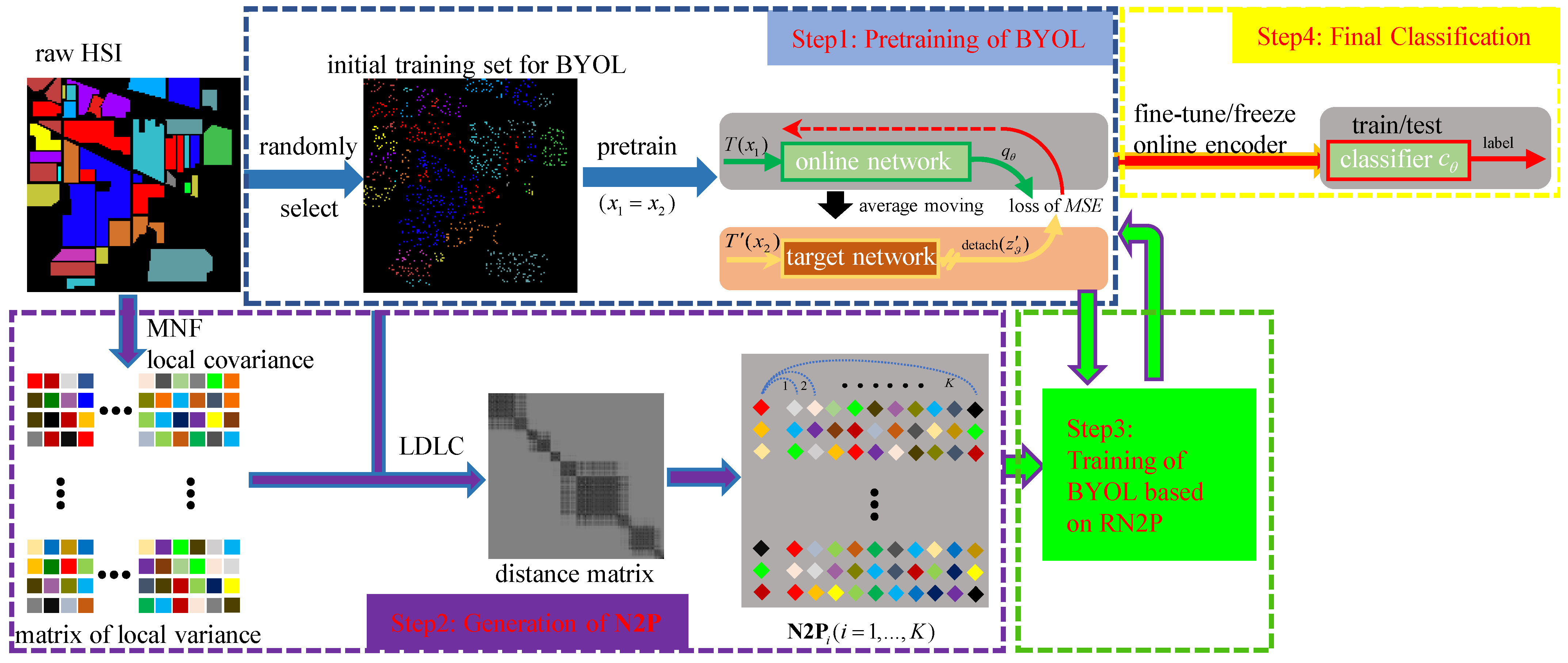
In this work, we, thus, tasked ourselves to find solutions to the above-mentioned two aspects, namely, exploiting discriminative information in the training process of S2L and fine-tuning from other HSIs. Aiming at the former aspect, we propose a n earest neighboring self-supervised learning (N2SSL) method for HSIC, based on the framework of BYOL and the well-known backbone of SSRN. To be specific, the proposed N2SSL method contains four main steps: pretraining of SSRN-based BYOL, generating nearest neighboring pairs (N2Ps) of samples derived from Log distance of local covariance (LDLC), training of BYOL based on reliable N2P (RN2P), final classification. First, a subset of all HSI samples is extracted as the initial training set to pretrain BYOL. Second, the affinity of these samples is generated by LDLC, and, thus, N2Ps can be easily constructed from each sample of the training set and one of its K-nearest neighboring samples. Third, extraction of RN2P and training of BYOL work in a collaborative way. In particular, N2P fed into BYOL with relatively smaller loss behave more similarly and, thus, can be treated as RN2P, whereas RN2P established by different samples are believed to help BYOL learn more discriminative representations and are, then, used to train BYOL. When the training process is finished, linear classification, based on frozen representation, is performed for final classification.

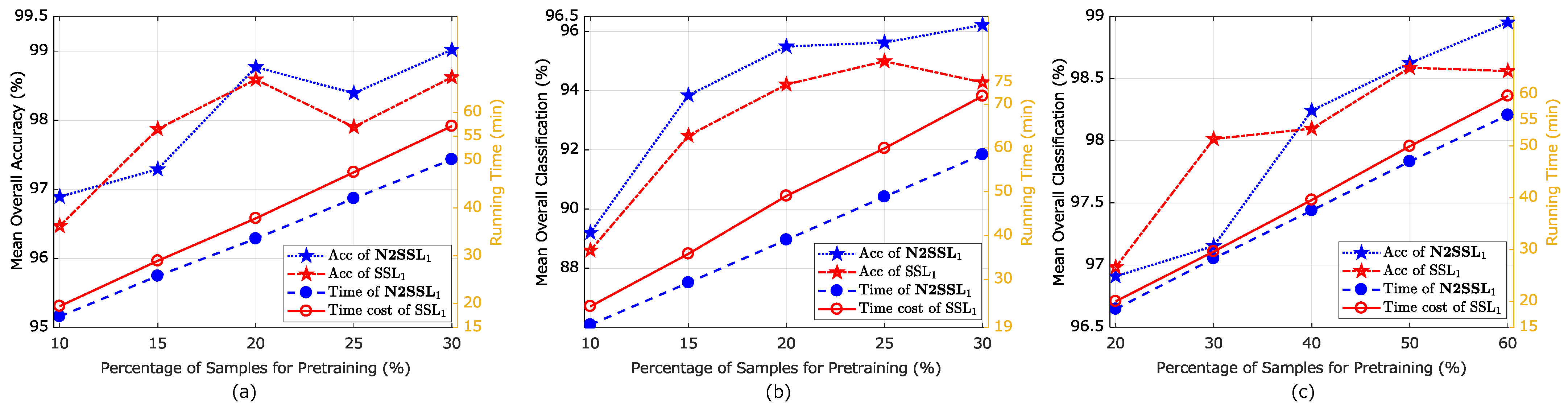
To understand the effect and importance of fine-tuning, we conducted an experimental study wherein N2SSL was performed on an unrelated HSI and then this was fine-tuned to another HSI; N2SSL was conducted on the Kennedy Space Center scene, but the learned network was then fine-tuned to University of Pavia and Indian Pines scenes. The classification accuracy and computational cost showed that the trained network from an unrelated HSI improved the efficiency.

The main contributions of our work are summarized as follows:

(1)

To the best knowledge of the authors, this is the first time that discriminative information, facilitating subsequent classification, is encoded by RN2P-based S2L. Comprehensive experiments on three benchmark HSIs were conducted to demonstrate the effectiveness of N2SSL, in terms of higher classification accuracy and less computational cost, compared to a standard framework of SSRN-based BYOL and other SOTA self-supervised methods designed for HSIC.

(2)

Fine-tuning of trained networks by N2SSL from an unrelated HSI to other HSIs is validated for the first time, which may be a new research topic of deep learning-based HSIC.

(3)

Since data augmentation (DA) plays a critical role in S2L, a comprehensive review of DA on HSI samples is illustrated in Section 2, which can be referred to by future S2L-based research on HSIs.

The rest of the paper is organized as follows. The DA of HSI samples and framework of BYOL are reviewed in Section 2. The proposed methodology of HSIC is presented in Section 3. Section 4 and Section 5 describe the experimental setup and results, respectively. Section 6 summarizes the research.

2. Background Algorithms

Given the different characteristics of HSI samples to those of natural images, DA techniques in HSI are usually derived from those used for computer vision, but show a lot of difference. Consequently, as they are critical to S2L, this section first provides a comprehensive review of DA techniques in HSI. Afterwards, a detailed introduction of BYOL is reported on.

2.1. DA of HSI

From the perspective of whether only labels are augmented, we divide DA techniques of HSI into two categories, i.e., only augment labels and augment samples (see

Table 1. Illustration of DA techniques for HSI.

Category		Ref.	Strategy of DA
Only augment labels		[47,48]	consistency of labels computed by local and global constraints (SAD and patch distances).
Augment samples	Self-augmentation	[49]	add Gaussian noise.
		[50]	convolutional transformation.
		[51]	shift the values in each band relatively to the average band value.
		[51]	multiply PCs by random factors.
		[52]	spatial random occlusion.
		[53,54]	rotate and flip.
		[55,56]	patch cleaning and imputation based on superpixels.
		[57]	different operations of rotate and flip on two windows.
	Mutual augmentation	[58]	consistency of labels of pixel-blocks that form a pair.
		[59,60]	mix-up.
		[61]	3D Cutmix and trainable spectral–spatial attention.
		[62]	weighting of nearest neighbors of central samples in local patch.
		[63]	clustering of samples in local patch.
		[64]	swapped replacement of cropped sub-patch.
	Synthetic augmentation	[65,66]	GAN.
		[67]	sampled from Gaussian mixture model fitted to each class.
		[68]	Hapke model.

). In order to augment labels, both Niu et al. [47] and Feng et al. [48] used consistency of labels computed by local and global constraints, where the only difference between them lies in the strategy of global constraint, e.g., spectral angular distances (SADs) and patch distances, respectively.

The augmentation of samples can be further categorized as self-augmentation, mutual and synthetic augmentation. As the name implies, self-augmentation indicates augmentation achieved by operation on each HSI sample itself, such as adding Gaussian noise [49] and applying convolutional transformation [50] to samples. Nalepa et al. proposed two ways for DA, i.e., shift the values in each band relative to the average band value and multiply principal components (PCs) by random factors [51]. Other works explored DA when samples behave as local patches, such as spatial random occlusion [52], rotate and flip [53,54], patch cleaning and imputation based on the border between superpixels [55,56]. Derived from the traditional augmentation technique, namely rotate and flip, Acción et al. applied heterogeneous operations of these two techniques on inner and outer patches [57].

Unlike self-augmentation, mutual augmentation of HSI samples works by exploiting several samples, e.g., mix-up, borrowed from machine learning literature [59,60], and consistency of labels of pixel and block that form pairs [58]. Along the lines of mix-up, Miao et al. applied 3D CutMix and trainable spectral–spatial attention module as DA to guide the CNN classifier to attend to the discriminative features of HSI [61]. Wang et al. proposed two strategies of weighting several nearest neighboring samples of the central sample as its augmentation, i.e., applying different sizes of patches and iteratively applying them to the new augmented image [62]. Similarly, Shang et al. iteratively augmented samples by a similar patch clustering strategy integrating Euclidean distance with SAD-based spatial–spectral metrics [63]. Operating on the level of local patch, Wang et al. replaced the removed regions with a cropped sub-patch from another sample belonging to different classes [64].

In addition to self-augmentation and mutual augmentation, synthetic augmentation works in a more abstract way by exploiting statistics of HSI samples or generative networks. For instance, Audebert et al. and Nalepa et al. investigated the capability of generative adversarial networks (GANs) to synthesize consistent labeled spectra [65,66]. Davari et al. generated synthetic data from a Gaussian mixture model fitted to each class of the training set [67], whereas Qin et al. incorporated prior knowledge of hyperspectral reflectance characteristics using the Hapke model for the augmentation of the training set [68].

2.2. BYOL

Figure 2 illustrates the framework of BYOL, composed of online and target networks. As previously described in Section 1, BYOL employs the addition of a predictor to the online network and applies an updating strategy of average moving to the target network to prevent collapsing.

Specifically, the online network contains three consecutive components: encoder $f_{\theta }$, projector $g_{\theta }$ and predictor $h_{\theta }$. The target network holds only encoder $f_{\vartheta }$ and projector $g_{\vartheta }$, having the same architectures as $f_{\theta }$ and $g_{\theta }$, respectively. The parameters of the target network ($\vartheta$) are the exponential moving averages of those of the online network ($\theta$). By denoting the momentum coefficient as m, usually set to 0.99 or 0.999, $\vartheta$ is updated after each training epoch as

$$\begin{array}{c}\hfill \vartheta \leftarrow m\vartheta +(1-m)\theta .\end{array}$$

(1)

Given image set $\mathcal{X}$ and two distributions of augmentations, i.e., $\mathcal{T}$ and ${\mathcal{T}}^{{}^{\prime }}$, two views of image $x\in \mathcal{X}$ can be computed by applying the respective augmentations, $T\sim \mathcal{T}$ and $T^{{}^{\prime }}\sim {\mathcal{T}}^{{}^{\prime }}$, to image x. From the perspective of network inference, the online network subsequently generates representation $r_{\theta }=f_{\theta }\left(T\left(x\right)\right)$ and projection $z_{\theta }=g_{\theta }\left(r_{\theta }\right)$, whereas the target network outputs representation $r_{\vartheta }^{{}^{\prime }}=f_{\vartheta }\left(T^{{}^{\prime }}\left(x\right)\right)$ and projection $z_{\vartheta }^{{}^{\prime }}=g_{\vartheta }\left(r_{\vartheta }^{{}^{\prime }}\right)$. Then, the final output of the online network is the prediction of $z_{\theta }$, i.e., $q_{\theta }=h_{\theta }\left(z_{\theta }\right)$. By respectively normalizing $q_{\theta }$ and $z_{\vartheta }^{{}^{\prime }}$ as $\overline{q_{\theta }}$ and ${\overline{z}}_{\vartheta }^{{}^{\prime }}$, the corresponding mean square error (MSE) is defined as

$$\begin{array}{c}\hfill {\mathcal{L}}_{\theta ,\vartheta }\triangleq \left|\right|\overline{q_{\theta }}-{\overline{z}}_{\vartheta }^{{}^{\prime }}{\left|\right|}_2^2=2-2·\frac{<q_{\theta },z_{\vartheta }^{{}^{\prime }}>}{\left|\right|q_{\theta }{\left|\right|}_2^2·\left|\right|z_{\vartheta }^{{}^{\prime }}{\left|\right|}_2^2},\end{array}$$

(2)

where $z_{\vartheta }^{{}^{\prime }}$ should be detached for stop-gradient. Moreover, two views of x are swapped to obtain the symmetric loss ${\mathcal{L}}_{\theta ,\vartheta }^{{}^{\prime }}$. With the learning rate $\eta$, $\theta$ is updated at each training epoch by performing a stochastic optimization step, as follows:

$$\begin{array}{c}\hfill \theta \leftarrow optimizer(\theta ,{\nabla }_{\theta }({\mathcal{L}}_{\theta ,\vartheta }+{\mathcal{L}}_{\theta ,\vartheta }^{{}^{\prime }}),\eta ).\end{array}$$

(3)

At the end of training, only the online encoder $f_{\theta }$ is kept to compute latent representations.

3. Proposed Methodology

As shown in Figure 3, the proposed N2SSL method consists of four main steps: (i) pretraining of BYOL, (ii) generation of nearest neighboring pairs (N2Ps), (iii) training of BYOL based on reliable N2P (RN2P) and (iv) classification. First, given the considerable computational load of self-supervised learning on all samples of one HSI, a subset of all HSI samples is randomly selected as the initial training set, i.e., $\mathbf{TS}=\{x_1,x_2,\dots ,x_{n_s}\}$, which is used to pretrain BYOL by applying different augmentations to each sample. Herein, we opted for simplicity and adopted the main backbone of SSRN as the encoder. Second, since it is expected to encode the discriminative information of HSI samples in the training process of BYOL, to facilitate subsequent classification, N2P is generated by using the Log-Euclidean distance of local covariance (LDLC). When LDLC between samples of TS is computed, each sample and one of its K-nearest neighboring compose a pair. For better illustration, the ith nearest neighboring samples and the corresponding HSI samples form the ith subset of N2P, i.e., N2P${}_i(i=1,\dots ,$ K). Third, since there failure in N2P may occur, i.e., pairs constructed by samples of different classes, the MSE-based loss of N2P, obtained by the pretrained BYOL is used to extract RN2P. Conversely, it is believed that training BYOL by RN2P can facilitate the learning discriminative information, as BYOL is forced to interact between augmentations of different, but similar, samples, instead of the same samples. Finally, linear classification, or fine-tuning-based labelling of samples is conducted. In the following, implementation details of the proposed method are described.

3.1. Pretraining of BYOL

Pretraining of BYOL is performed by learning on two augmentations of each sample in TS. Specifically, the three components of the online network are the SSRN-based encoder $f_{\theta }$, two networks of multilayer perceptrons (MLPs) working as projector $g_{\theta }$ and predictor $h_{\theta }$, respectively. The target encoder $f_{\vartheta }$ and projector $g_{\vartheta }$ share the same architecture as $f_{\theta }$ and $g_{\theta }$, respectively. 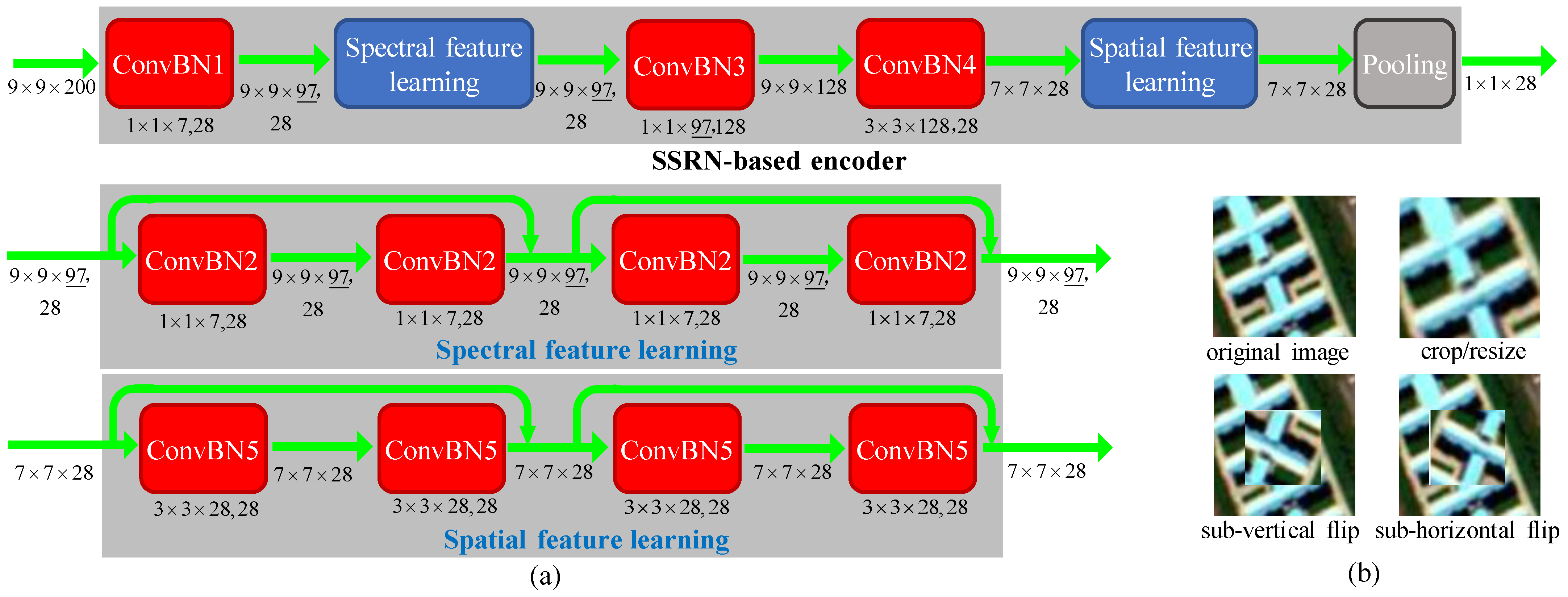Figure 4a gives an example of an SSRN-based encoder that extracts deep features via two residual modules of spectral and spatial feature learning. Please refer to [7] for details of SSRN. For simple illustration, we herein take a 3-D sample of the Indian Pines image with 200 bands as an example. The neighboring region of 9 × 9 pixels surrounding each pixel is considered to be the 3-D sample for the central pixel with the size of 9 × 9 × 200. The 3-D cube is first convolved by 281 × 1 × 7 spectral kernels (ConvBN1) with a subsampling stride of (1, 1, 2) to generate 289 × 9 × 97 cubes. Then, the module of spectral feature learning employs four convolutional layers (ConvBN2) and two identity mappings to learn the deep spectral features. All of the four convolution kernels share the same size of 281 × 1 × 7 with padding to keep the same size of output as input. Subsequently, two convolutional layers (ConvBN3 and ConvBN4) are employed to abstract spectral and spatial features, respectively. Following ConvBN4, the module of spatial feature learning uses four successive 3-D convolutional filter banks (ConvBN5), where the kernels have the same depth as the input 3-D feature volume. Similarly, the outputs of these filter banks keep the same size as the inputs of the feature cubes. Finally, an average pooling layer generates a 1 × 1 × 28 feature vector. When the size of input 3-D cube is fixed, the only parameter of the SSRN-based encoder is the kernel size of ConvBN3, i.e., the value of 97 underlined, which is determined by the number of bands. Furthermore, the sizes of MLP networks of the projectors ($g_{\theta }$ and $g_{\vartheta }$) and predictor $h_{\theta }$ were set to 28-512-128 and 128-512-128, respectively.

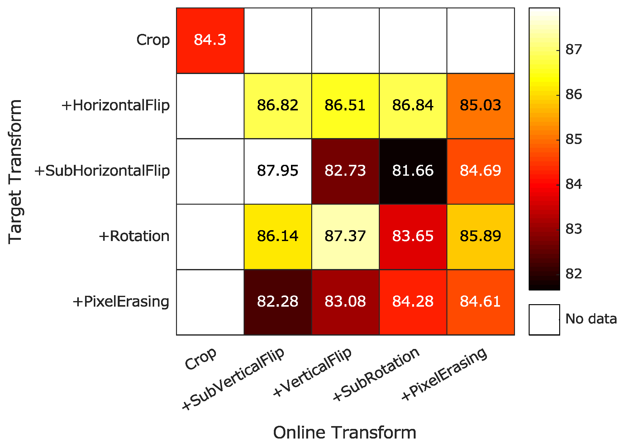
Regarding the augmentations used in BYOL, random cropping, followed by resizing back to the original size, was employed as it has proved to be effective in processing 3-D HSI samples. Empirically, we conducted experiments related to classification accuracy with respect to different augmentations. It was found that random cropping, followed by resizing with sub-vertical flip and with sub-horizontal flip, were enough for the online and target networks, respectively. Specifically, given one image pair of 9 × 9 × b, where b is the number of bands, a random spatial patch of each image was selected, with an area uniformly sampled between 8% and 100% of that of the original image, and an aspect ratio logarithmically sampled between $\frac{3}{4}$ and $\frac{4}{3}$. This patch was then resized to the original size of 9 × 9$\times$ b using bicubic interpolation. For the optional sub-horizontal and sub-vertical flips, a sub-window surrounding the central pixel was randomly set to 3 × 3 to 7 × 7 pixels. Figure 4b illustrates a conceptual example of these transforms. By applying MSE-based loss in Equation (2) on augmented TS, pretraining of BYOL was easily achieved in $n_{e1}$ epochs.

3.2. Generatation of N2P

As mentioned above, two samples from one pair are expected to belong to the same category for encoding discriminative information for BYOL training. Thus, metrics, or UFE methods, achieving SOTA performance of computing affinity between HSI samples are considered to be candidates for the generation of N2P. Among these methods, local covariance matrix representation, exploiting spectral–spatial information, has been successfully applied to both unsupervised and supervised HSIC [24,25,69]. Compared with SAM and Euclidean distances, it exploited the similarities and variances of local samples and proved to be suitable for measuring distances between HSI samples. Consequently, we employed it for generation of N2P, which computed the Log-Euclidean distances of local covariance (LDLC) of similar samples.

Particularly, maximum noise fraction (MNF) was first applied to the original HSI to reduce the dimensionality and suppress noise. Given the window size T, the SAD measure was used to find the M-1 most similar neighboring samples of the central sample. Then, these M samples were treated as a local set, i.e., P = {$x_i(i=1,\dots ,M)$}. Then, the covariance of P was formulated as

$$\begin{array}{c}\hfill {\mathbf{C}}_{\mathbf{P}}=\frac{1}{M-1}\sum _{i=1}^N(x_i-{\mu }_{\mathbf{P}}){(x_i-{\mu }_{\mathbf{P}})}^{\mathrm{T}},\end{array}$$

(4)

where ${\mu }_{\mathbf{P}}$ denotes the mean of samples. As covariance matrices are symmetric positive definites, they lie on a Riemannian manifold and, thus, Euclidean distance is hardly suitable for them, whereas LDLC was proposed in [70] to model the differences of covariance matrices. Given two sets ${\mathbf{P}}_1$ and ${\mathbf{P}}_2$ corresponding to samples $x_1$ and $x_2$, the corresponding covariance matrices are denoted as ${\mathbf{C}}_{{\mathbf{P}}_1}$ and ${\mathbf{C}}_{{\mathbf{P}}_2}$, respectively. The LDLC between the two samples is then defined as

$$\begin{array}{c}\hfill {dis}_{\mathrm{LDLC}}(x_1,x_2)=\frac{0.5\times \mathbf{var}(v_1-v_2)}{\mathbf{var}\left(v_1\right)+\mathbf{var}\left(v_2\right)}\end{array}$$

(5)

where var denotes the vector variance and $v=vec(\mathrm{logm}\left({\mathbf{C}}_{\mathbf{P}}\right)$ represents the vector of CM logarithm on the set $\mathbf{P}$. The main parameters are the number of MNF components L, the number of neighboring samples M and the window size T, which were set to 20, 25 and 220, respectively.

With the definition of LDLC, the distances among all samples in TS can be computed. Afterwards, each sample and one of its K-nearest neighboring samples formed the subset N2P${}_i(i=1,\dots ,$ K) and, thus, K$n_s$ pairs were generated.

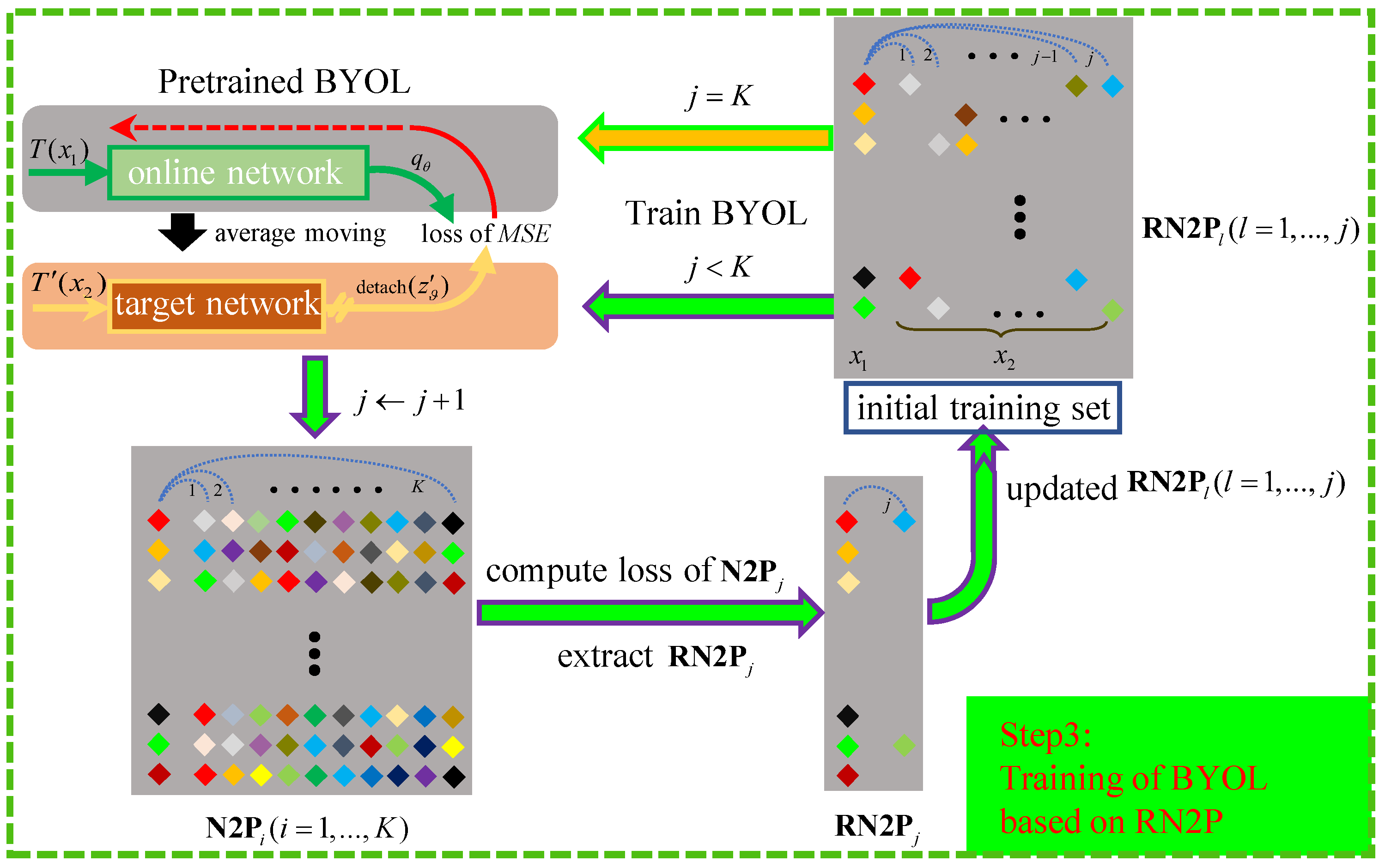
3.3. Training of BYOL Based on RN2P

By learning between two views of one sample, pretrained BYOL is expected to learn the latent semantic representations of HSI samples. Therefore, when two views of different samples belonging to the same category are fed into BYOL, the corresponding MSE-based loss is expected to be relatively small. Based on this observation and the truth that the original N2P can hardly be accurate enough, pretrained BYOL can be used for further refinement of N2P, i.e., extraction of RN2P. Since N2P is obtained via LDLC-based distances between nearest neighboring samples, N2P${}_i$ is believed to be more reliable than N2P${}_j$ ($j>i$). Thus, N2P${}_i$ ($i=1,\dots ,$ K) was used to extract RN2P${}_i$ ($i=1,\dots ,$ K) in order. Meanwhile, RN2P${}_i$ is naturally beneficial to extract RN2P${}_j$ ($j>i$) when it is used to train BYOL. The strategy is similar to the concept of evolving, i.e., the network learns semantic representation from easy pairs to hard pairs gradually, which has been applied to several applications, such as clustering of natural images. Consequently, extracted RN2P was added to TS to train BYOL for further extracting of RN2P. Once the extraction of RN2P finished, they were used to train BYOL for $n_{e3}$ epochs.

In detail, as shown in Figure 5, we constantly computed the MSE-based loss of N2P${}_j$ and extracted pairs with the smallest losses as RN2P${}_j$, according to the ratio, i.e., $\frac{1}{K}$. In this way, RN2P${}_j$ contained $\frac{n_s}{K}$ pairs and was added to the training set. Then, BYOL was trained by the new training set with $n_{e2}$ epochs and used for generation of RN2P${}_{j+1}$. Thus, when the iteration process finished, RN2P${}_j(j=1,\dots ,$ K) containing $n_s$ pairs were used to perform subsequent training of BYOL for $n_{e3}$ epochs. The implementation details of the proposed iterative process are illustrated in Algorithm 1.

Algorithm 1: Training of BYOL based on RN2P.

Input:

pretrained networks and N2P, initial training set: TS, number of epochs: ne2, number of final epochs: ne3, ratio for extracting RN2P: $\eta =\frac{1}{K}$.

1: Repeats:

2:   Compute MSE-based loss of N2Pj.

3:   Extract RN2Pj according to η.

4:   Train BYOL using TS and RN2Pl (l = 1, …, j) for ne2 epochs.

5:   j ← j + 1.

6: Until all N2Pj is processed.

7: Train BYOL using RN2P for ne3 epochs.

Return: trained BYOL.

3.4. Final Classification

When training of BYOL was over, only the online encoder $f_{\theta }$ was kept to compute the latent representations of both labeled and unlabeled HSI samples. Then, the corresponding classifier was designed as an MLP network of 28-C, where C was the number of classes. We regularized the classifier by clipping the logits using a hyperbolic tangent function

$$\begin{array}{c}\hfill tclip\left(r_l\right)\triangleq \alpha ·tanh(r_l/\alpha ),\end{array}$$

(6)

where $\alpha$ is a positive scalar and $r_l$ is the output of the classifier on labeled samples, and by adding a logit-regularization penalty term in the loss

$$\begin{array}{c}\hfill loss(r_l,y)\triangleq \mathcal{L}(tclip\left(r_l\right),y)+\beta ·average(tclip{\left(r_l\right)}^2),\end{array}$$

(7)

where $\mathcal{L}$ is the cross-entropy function, y denotes the labels of labeled samples, and $\beta$ is the regularization parameter. We set $\alpha =20$ and $\beta =1.0\times {10}^{-2}$ as [39].

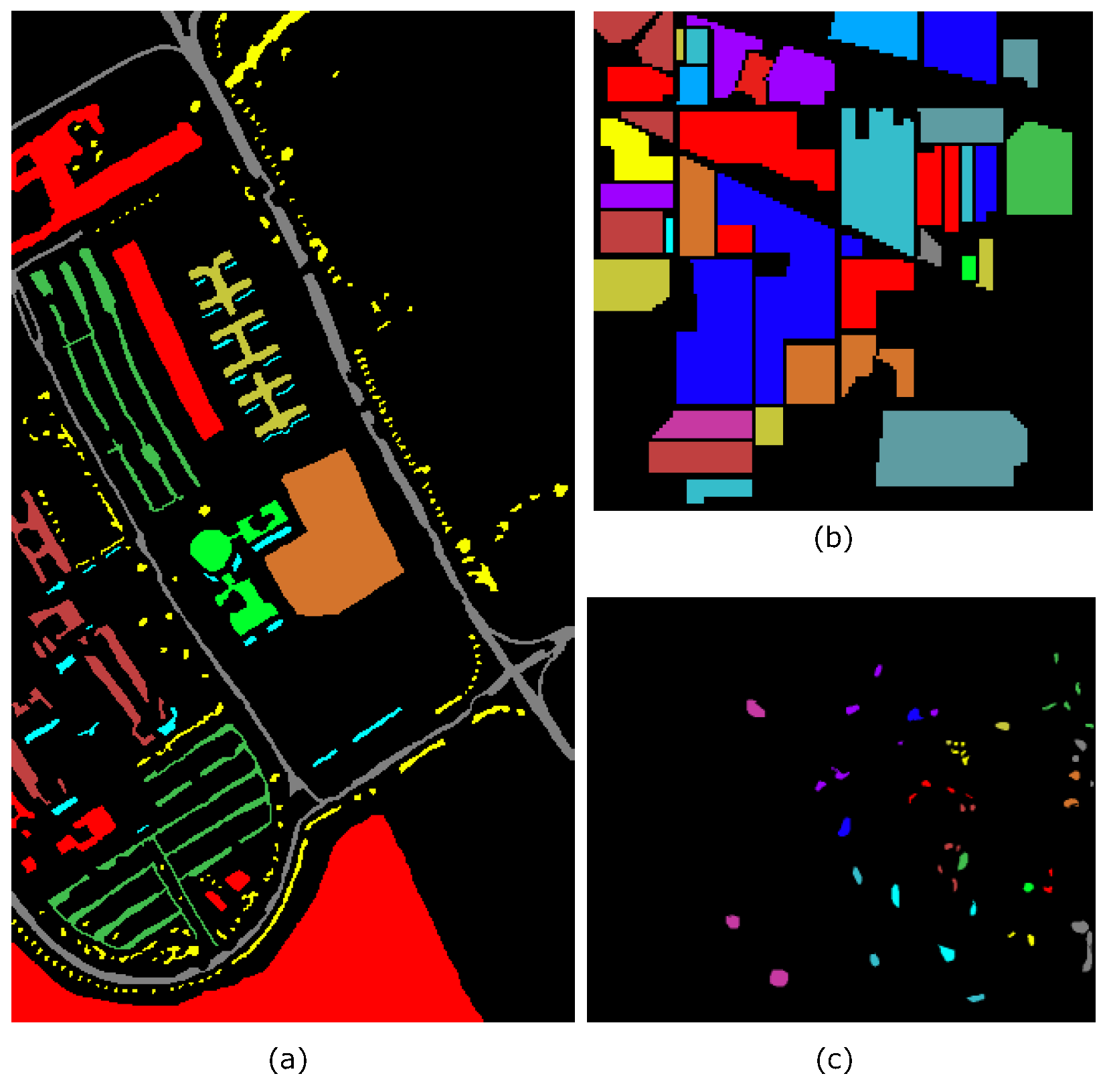
In the case of linear classification, the parameters of the online encoder are fixed and only the classifier is trained. Instead, both the online encoder and classifier are trained in the case of fine-tuning. Finally, the classification map was obtained by the inference of all samples of HSI.

4. Experimental Datasets and Setup

4.1. Dataset Descriptions

We evaluated the proposed N2SSL method by using three publicly available benchmark HSIs, i.e., the University of Pavia (UP), Indian Pines (IP) and Kennedy Space Center (KSC) scenes. The UP scene is an image collected by the reflective optics spectrographic image system over the University of Pavia. It contains 103 spectral reflectance bands of 610 × 340 pixels, covering 9 classes of interest. The IP scene is an Indian Pines image captured by an airborne visible infrared imaging spectrometer (AVRIS), which contains 200 bands of 145 × 145 pixels. As seen from

Table 2. Number of samples available for UP, IP and KSC scenes.

UP		IP		KSC
Class	GT	Class	GT	Class	GT
Asphalt	6851	Alfalfa	46	Scrub	761
Meadows	18,686	Corn-notill	1428	Willow swamp	243
Gravel	2207	Corn-min	830	CP hammock	256
Trees	3436	Corn	237	Slash pine	252
Metal sheets	1378	G-pasture	483	Oak/Broadleaf	161
Bare soil	5104	G-trees	730	Hardwood	229
Bitumen	1356	G-pasture-m	28	Swamp	105
Bricks	3878	H-windrowed	478	G-march	431
Shadow	1026	Oats	20	Sp-marsh	520
		Soybean-n	972	C-marsh	404
		Soybean-m	2455	Sa-marsh	419
		Soybean-c	593	Mud flats	503
		Wheat	205	Water	927
		Woods	1265
		B-Grass	386
		Stone-Steel	93

The colors correspond to the classes in Figure 6.

, its 16 different classes represent mostly different types of vegetation. The KSC scene is an image acquired by the AVIRIS sensor over the Kennedy Space Center with a spatial resolution of 18 m. It covers 13 classes of 512 × 614 pixels with 176 bands after removing water absorption. Table 2 and Figure 6 report the quantitative and qualitative ground truths(GTs) of the three scenes, respectively.

4.2. Experimental Setup

4.2.1. Implementation Details

•

Architecture: We used SSRN-based encoders as $f_{\theta }$ and $f_{\vartheta }$, with kernel sizes of ConvBN3 set to 49, 97 and 85 for UP, IP and KSC scenes, respectively. The projectors ($g_{\theta }$ and $g_{\vartheta }$) and predictor $h_{\theta }$ were set to 28-512-128 and 128-512-128 MPL networks for all scenes, respectively. For the target network, the exponential moving average parameter was fixed as 0.996 in both pretraining and training process.

•

Typical Baseline: To fairly illustrate the improvement brought by learning between augmentations of RN2P, we employed BYOL that only learnt from augmentations of the same samples as a baseline in all experiments. From the perspective of N2SSL, we directly denoted it as SSL for consistency. Since final classification could be achieved by learning on the frozen features, or fine-tuning the learned encoder, we denoted them with different subscripts. Specifically, SSL${}_1$ and N2SSL${}_1$ represent linear classification, whereas SSL${}_2$ and N2SSL${}_2$ represent classification via fine-tuning.

Regarding the case of fine-tuning, we chose to fine-tune the online encoder trained on the KSC scene to both UP and IP scenes due to the following considerations. First, compared with the UP and IP scenes, the KSC scene had less samples. In other words, the online encoder was trained on a relatively small HSI, but fine-tuned to large HSIs, which is more similar to practical hyperspectral applications. Second, since the number of bands of the KSC scene was larger than that of the UP scene and smaller than that of the IP scene, up-sampling and down-sampling of spectral channels had to be conducted for the UP and IP scenes, respectively. In this way, both operations of up-sampling and down-sampling were achieved. The combined analysis of both UP and IP scenes eliminated the effect brought by inevitable up-sampling or down-sampling of spectral channels, making the results more convincing. Specifically, the spectral channels of the UP and IP scenes were linearly interpolated to be the same as the KSC scene. For simplicity, these two cases were denoted as KSC→UP and KSC→IP, respectively.

•

Optimization: For rationale of comparison between SSL and N2SSL methods, they held the same optimization setting for each scene, i.e., batch-size and learning rate (LR) in

Table 3. Learning rate and training epochs of SSL and N2SSL methods for all the scenes.

Dataset	Learning Rate	Batch Size	Number of Epochs
			SSL	N2SSL
				${\mathit{n}}_{\mathit{e}\mathbf{1}}$	${\mathit{n}}_{\mathit{e}\mathbf{2}}$	${\mathit{n}}_{\mathit{e}\mathbf{3}}$
UP	cosine decay schedule with a warm-up of 10 epochs.	128	100	40	2	30
IP		32	200	80	4	60
KSC		32	200	80	2	90

. Note that both of them were empirically determined according to several trials. In particular, the initial and largest LRs of cosine decay schedule were 1.0 × ${10}^{-3}$ and 2.5 × ${10}^{-2}$, respectively, with a warm-up period of 10 epochs. The SGD optimizer with momentum of 0.9 and weight decay of 4.0 × ${10}^{-4}$ was employed. Moreover, a cosine decay schedule of N2SSL was only applied to the pretraining and final training processes, whereas for the iterative process of extracting RN2P, the learning rate remained unchanged. In this way, the dynamic LR of N2SSL was the same as that of SSL.

For epochs of N2SSL, we empirically set them to ensure computational cost less than the corresponding SSL method for each scene (see $n_{e1},n_{e2},n_{e3}$ in Table 3). For linear classification, LR and number of training epochs for the classifier were set to 2.0 × ${10}^{-3}$ and 4000, respectively. For the cases of both KSC→UP and KSC→IP, the LRs for the encoder and the classifier were set to 2.0 × ${10}^{-4}$ and 2.0 × ${10}^{-3}$, respectively. Both of them degraded by 2 with a patience of 10 epochs on the decrease of training loss. The total number of fine-tuning epochs for all scenes was set to 200.

•

Specific Parameters of N2SSL: Number of nearest neighboring samples, i.e., K, was set to 20. The percentages of samples for pretraining were set to 20%, 20% and 40% for the three scenes, respectively.

4.2.2. Other Baseline Methods

In order to draw a general comparison, UFE, DL-based supervised classification and self-supervised approaches were employed as baseline methods:

•

MSuperPCA [14]: MSuperPCA (https://github.com/junjun-jiang/SuperPCA (accessed on 15 March 2023)) is a conventional UFE method that applied superpixel-wise PCA to HSI.

•

S3-PCA [15]: S3-PCA (https://github.com/XinweiJiang/S3-PCA (accessed on 15 March 2023)) adopted superpixels-based local reconstruction to filter the HSIs and used the PCA-based global features as the supplement of local features.

•

HybridSN [10]: HybridSN (https://github.com/gokriznastic/HybridSN (accessed on 15 March 2023)) is a state-of-the-art supervised DL method that exploited both 3-D spectral–spatial features and 2-D abstract-level spatial representation.

•

$SSRN$ [7]: SSRN (https://github.com/zilongzhong/SSRN (accessed on 15 March 2023)) is a typical residual CNN designed for HSIC and worked as the encoder of BYOL in our method.

•

$SSTN$ [11]: SSTN (https://github.com/zilongzhong/SSTN(accessed on 15 March 2023)) combines spatial attention and spectral association modules to overcome the constraints of convolution kernels.

•

ContrastNet [43]: ContrastNet integrates the popular prototypical contrastive learning with data augmentations achieved by two different autoencoders, i.e., variational autoencoder and adversarial autoencoder.

•

CL-Transformer [42]: CL-Transformer explores the capability of BYOL-based S2L on HSIC based on the backbone of the transformer.

•

SSCL [44]: SSCL pays more attention to the data preprocessing of HSI and uses Gaussian noise for augmentation.

•

S3FN [45]: S3FN uses feature transformation to obtain two feature descriptions of the same source data from different views and proposes the spectral–spatial feature learning network to conduct contrastive learning.

•

Self-supervised learning with adaptive distillation (SSAD) [34]: SSAD applies self-supervised information to train the network by knowledge distillation, where self-supervised knowledge is the adaptive soft label generated by spatial—spectral similarity measurement.

The typical baseline methods (MSuperPCA, S3-PCA, HybridSN, SSRN and SSTN) were employed for all three scenes by reproducing the classification via the corresponding publicly available codes. The parameters of support vector machine in MSuperPCA and S3-PCA were tuned to achieve the best classification performance. Similarly, for Hybrid, SSRN, SSTN, SSL and N2SSL, highest accuracies were reported in the training process of classifiers. Regarding self-supervised methods, we compared both N2SSL${}_1$ and N2SSL${}_2$ with them under the same setting of labeled samples for each scene. For each setting of a number of labeled samples, 20 trials of the classification were conducted to report relatively stable performance. To numerically evaluate the accuracy, overall accuracy (OA), corresponding average accuracy (AA) and Kappa statistics ($\mathcal{K}$) were used. Furthermore, the running time consumed per trial was employed to describe the computational load. All our experiments were conducted using Matlab R2017b and Pytorch on a workstation equipped with an Intel(R) Xeon(R) Gold 6254 CPU, 16 GB of RAM and a Tesla V100 GPU with 32-GB memory.

5. Experimental Results

5.1. Results of Linear Classification

5.1.1. Comparison between SSL${}_1$ and N2SSL${}_1$

Different from the setting of labeled samples for analysis of parameter setting, we explored more deeply the capability of SSL${}_1$ and N2SSL${}_1$ for HSIC of three scenes using various settings of labeled samples, i.e., ranging from 6 to 10 per class for imbalance testing and ranging from 100 to 600 in total. Note that, for the case of 100 to 600, the number of labeled samples per class was determined by the relative ratios of different classes.

Table 4. Comparison of mean OAs obtained by SSL${}_1$ and N2SSL${}_1$ for all the three scenes with different numbers of labeled samples.

Train#		6	7	8	9	10	100	200	300	400	500	600
UP	SSL${}_1$	92.014 ± 3.80	92.691 ± 3.27	93.716 ± 3.07	93.681 ± 3.04	94.536 ± 2.86	97.448 ± 0.94	98.589 ± 0.46	98.938 ± 0.33	99.112 ± 0.24	99.205 ± 0.21	99.268 ± 0.19
	N2SSL${}_1$	89.909 ± 4.16	91.070 ± 3.54	91.706 ± 3.56	92.169 ± 3.38	92.795 ± 3.15	97.123 ± 1.08	98.769 ± 0.49	99.203 ± 0.28	99.304 ± 0.18	99.416 ± 0.18	99.487 ± 0.15
IP	SSL${}_1$	83.440 ± 3.10	84.863 ± 3.04	86.046 ± 3.10	87.087 ± 2.72	88.832 ± 2.69	89.716 ± 2.14	94.207 ± 1.12	95.781 ± 0.62	96.284 ± 0.61	96.776 ± 0.53	97.135 ± 0.41
	N2SSL${}_1$	86.250 ± 3.36	87.223 ± 2.99	88.003 ± 3.03	89.359 ± 2.05	90.742 ± 2.19	92.025 ± 1.80	95.490 ± 0.96	96.486 ± 0.51	97.046 ± 0.45	97.392 ± 0.35	97.697 ± 0.26
KSC	SSL${}_1$	95.348 ± 2.23	95.851 ± 1.79	96.536 ± 1.35	96.859 ± 1.26	97.238 ± 1.08	96.004 ± 1.57	98.097 ± 0.56	98.698 ± 0.38	98.976 ± 0.25	99.133 ± 0.20	99.229 ± 0.23
	N2SSL${}_1$	95.546 ± 2.45	96.055 ± 1.86	96.617 ± 1.34	96.873 ± 1.14	97.287 ± 1.03	96.326 ± 1.59	98.243 ± 0.58	98.872 ± 0.43	99.199 ± 0.27	99.415 ± 0.24	99.478 ± 0.23

reports the mean OAs and the corresponding standard errors. The following observations were easily obtained.

(1)

The increasing trend of mean OAs confirmed that 20 trials were enough to achieve stable results. Moreover, standard errors of OAs for small numbers of labeled samples appeared to be higher.

(2)

SSL${}_1$ easily yielded better performance than N2SSL${}_1$ for the UP scene when the number of labeled samples ranged from 6 to 10 per class, or equaled 100 in total. In particular, when numbers of labeled samples were 10 per class and 100 in total, the accuracies achieved by SSL${}_1$ were 94.536% and 97.488%, respectively, 1.741% and 0.325% higher than that of N2SSL${}_1$. Since 10 per class meant 90 in total for the UP scene, it could be roughly concluded that the N2SSL${}_1$ method was more sensitive than the SSL${}_1$ method to imbalances between labeled and testing samples of each class. When comparing the results of the KSC scene, using 8 per class and 100 in total, a similar conclusion was observed.

(3)

The mean OAs of N2SSL${}_1$ for the IP and KSC scenes with various numbers of labeled samples were in the range of 86.250–97.697% and 95.546–99.478%, respectively, which was always higher than those of SSL${}_1$, i.e., in the range of 83.440–97.135% and 95.348–99.229%, respectively. A similar trend was found for the UP scene when there were no less than 200 labeled samples.

One may notice that the superiority of N2SSL${}_1$ over SSL${}_1$ became more apparent in the IP scene. To give a qualitative comparison, Figure 7 illustrates the t-distributed stochastic neighbor embedding (t-SNE) feature visualization of frozen deep features of the online encoder for the IP scene (C5, C7, C10 and C15). Compared with SSL${}_1$, it is clear that better separation between classes was achieved with the learned features by N2SSL${}_1$, such as “Soybean-n” (C10) and “B-Grass” (C15) in ellipses, “G-pasture” (C5) and “G-pasture-m” (C7) in rectangles. Consequently, interacting between nearest neighboring samples in N2SSL${}_1$ facilitated the online encoder in learning more discriminative features.

5.1.2. Comparison with SOTA UFE and DL Methods

Table 5. Classification results of SOTA methods, SSL${}_1$ and N2SSL${}_1$ by selecting 200 training samples on the UP scene.

No.	Train#	Test#	MSuperPCA	S3PCA	HybridSN	SSRN	SSTN	SSL${}_1$	N2SSL${}_1$
C1	31	6600	94.92	96.51	89.40	97.34	97.92	99.56	98.43
C2	88	18,561	99.09	99.43	98.96	98.57	99.58	99.92	99.92
C3	10	2089	82.28	93.99	77.50	81.36	88.61	92.46	95.30
C4	13	3051	49.68	76.99	77.67	94.69	91.89	94.27	96.97
C5	8	1337	81.22	99.19	99.45	99.71	99.40	99.97	99.99
C6	23	5006	87.65	97.40	96.42	95.13	98.52	99.21	99.69
C7	9	1321	94.97	93.71	95.84	96.36	97.21	99.85	99.98
C8	14	3668	91.49	97.16	77.74	94.01	93.03	95.80	95.46
C9	4	943	32.78	89.97	37.22	99.48	95.39	97.00	96.44
All	OA (%)		89.92 ± 1.51	96.27 ± 0.60	91.32 ± 1.29	96.45 ± 0.92	97.37 ± 0.52	98.59 ± 0.46	98.77 ± 0.49
	AA (%)		79.34 ± 4.45	93.82 ± 1.15	83.36 ± 2.10	95.18 ± 1.13	95.73 ± 1.03	97.56 ± 0.69	98.02 ± 0.64
	$\mathcal{K}$ (%)		86.25 ± 2.13	95.02 ± 0.81	88.45 ± 1.71	95.29 ± 1.21	96.51 ± 0.69	98.13 ± 0.61	98.37 ± 0.65
Time (min)			2.10	2.97	5.95	27.32	16.88	38.16	33.87

The best results are reported in bold.

,

Table 6. Classification results of SOTA methods, SSL${}_1$ and N2SSL${}_1$ by selecting 200 training samples on the IP scene.

No.	Train#	Test#	MSuperPCA	S3PCA	HybridSN	SSRN	SSTN	SSL${}_1$	N2SSL${}_1$
C1	2	44	0.00	5.00	72.61	81.82	82.16	87.50	91.82
C2	27	1401	88.72	90.68	72.76	81.41	92.16	92.18	93.47
C3	19	811	90.33	92.52	71.58	87.02	93.97	93.98	93.63
C4	4	233	42.73	53.76	42.73	72.21	82.30	76.22	74.08
C5	9	474	93.07	93.63	76.61	88.34	87.69	90.37	89.92
C6	14	716	97.16	97.19	95.09	95.44	96.89	94.16	99.27
C7	2	26	0.00	0.00	97.12	97.88	98.08	99.62	98.08
C8	10	468	99.73	100.00	99.85	97.30	99.81	99.86	99.96
C9	3	17	99.12	91.18	99.41	99.41	98.53	97.65	98.82
C10	24	948	93.11	94.10	82.26	88.82	90.78	92.42	94.49
C11	41	2414	97.92	96.09	86.89	91.07	94.93	95.41	96.23
C12	14	579	84.61	85.63	67.25	83.02	93.15	94.05	96.18
C13	4	201	99.50	99.18	92.46	97.99	98.48	96.99	99.03
C14	18	1247	99.27	97.68	93.62	97.67	98.46	98.91	99.82
C15	7	379	91.99	92.68	69.63	75.84	86.81	91.33	95.03
C16	2	91	2.47	2.58	72.31	95.11	89.34	94.89	95.99
All	OA (%)		91.76 ± 1.08	92.05 ± 1.97	81.94 ± 1.64	89.17 ± 1.51	93.81 ± 0.85	94.21 ± 1.12	95.49 ± 0.96
	AA (%)		73.73 ± 1.26	74.49 ± 3.03	80.76 ± 2.26	89.40 ± 2.19	92.72 ± 1.18	93.47 ± 1.15	94.74 ± 1.05
	$\mathcal{K}$ (%)		90.52 ± 1.24	90.90 ± 2.24	79.36 ± 1.87	87.64 ± 1.73	92.95 ± 0.97	93.39 ± 1.27	94.86 ± 1.09
Time (min)			0.90	0.13	1.59	15.10	6.38	48.05	39.07

The best results are reported in bold.

and

Table 7. Classification results of SOTA methods, SSL${}_1$ and N2SSL${}_1$ by selecting 200 training samples on the KSC scene.

No.	Train#	Test#	MSuperPCA	S3PCA	HybridSN	SSRN	SSTN	SSL${}_1$	N2SSL${}_1$
C1	29	732	98.29	99.60	88.90	98.01	99.82	99.93	100.00
C2	9	234	94.55	91.90	57.80	91.39	93.91	95.28	94.10
C3	10	246	92.09	94.86	76.10	98.25	96.36	99.19	99.72
C4	10	242	92.71	93.24	51.43	76.96	83.35	92.64	92.93
C5	6	155	89.29	88.52	76.06	78.84	65.29	79.87	82.03
C6	9	220	93.73	80.89	72.39	85.32	95.93	97.70	99.91
C7	4	101	100.00	90.64	61.58	95.69	86.49	90.69	94.70
C8	17	414	95.00	98.56	84.96	96.63	97.79	99.19	98.66
C9	20	500	99.76	99.56	89.17	98.79	99.35	99.74	98.69
C10	16	388	92.11	86.48	60.05	95.66	98.87	99.83	99.39
C11	16	403	99.35	99.64	76.59	98.76	98.81	99.93	100.00
C12	19	484	96.59	96.02	77.35	96.73	96.43	97.37	98.22
C13	35	892	98.71	98.39	99.13	99.99	100.00	100.00	100.00
All	OA (%)		96.49 ± 0.74	95.69 ± 0.90	80.52 ± 3.14	95.57 ± 1.05	96.41 ± 1.43	98.10 ± 0.56	98.24 ± 0.58
	AA (%)		95.55 ± 1.01	93.72 ± 2.04	74.73 ± 3.80	93.15 ± 1.64	93.26 ± 2.50	96.26 ± 1.04	96.80 ± 1.06
	$\mathcal{K}$ (%)		96.09 ± 0.82	95.20 ± 1.01	78.24 ± 3.52	95.07 ± 1.17	96.00 ± 1.60	97.88 ± 0.62	98.04 ± 0.64
Time (min)			1.55	5.36	2.92	8.85	5.01	39.75	37.60

The best results are reported in bold.

report the mean quantitative evaluation of different methods in terms of individual class accuracies, OA, AA, $\mathcal{K}$ and running time using 200 labeled samples for the UP, IP and KSC scenes, respectively. The following observations can be easily drawn:

(1)

Among these seven methods, N2SSL${}_1$ achieved the best classification accuracies, with mean OA 0.18%, 1.28% and 0.14% higher than those of SSL${}_1$ for the UP, IP and KSC scenes, respectively. Meanwhile, the running time of the N2SSL${}_1$ method averaged 5.14 min less than that of the SSL${}_1$ method.

(2)

Looking at individual accuracy of each class, N2SSL${}_1$ delivered the best performance for most classes of the three scenes. As shown in Figure 7 and as stated above, t-SNE computed by N2SSL${}_1$ of “Stone-Steel” (C16) and “Soybean-c” (C12), “Soybean-n” (C10) and “B-Grass” (C15) in the IP scene showed better separation. In particular, the same quantitative results can be found in Table 6, i.e., accuracies of C10, C12, C15 and C16 were 2.01%, 2.14%, 3.70% and 1.10% higher than those achieved by SSL${}_1$, respectively (see the underlined accuracies).

(3)

HybridSN was inferior to other methods, resulting in the lowest mean OAs of 81.94% and 80.52% for the IP and KSC scenes, respectively, whereas MSuperPCA delivered the worst accuracy for the UP scene with a mean OA of 89.92%.

(4)

Compared with SSRN that shares the same architecture with SSL${}_1$ and N2SSL${}_1$, large improvements on OA, AA and $\mathcal{K}$ were found for all scenes, validating the success of self-supervised learning on nearest neighboring samples. In particular, mean OAs achieved by N2SSL${}_1$ averaged 2.32%, 6.32% and 2.67% higher for the three scenes, respectively.

(5)

Compared with SSTN based on framework of Transformer, CNN-based N2SSL${}_1$ still held an advantage on accuracies for all scenes. However, the corresponding running time was also higher than that of SSTN.

(6)

Regarding computational time, conventional methods (MSuperPCA and S3PCA) took the least time for all scenes, whereas SSL${}_1$ and N2SSL${}_1$ required much more time, due to the training of BYOL.

In order to qualitatively display the mean classification maps, the average accuracy of each sample in the HSI was computed and then transformed to intensity. For example, when the average accuracy over 20 trials was 100%, its intensity was set as 1. On the other hand, the intensity was set as 0 if the sample was never correctly classified. Figure 8, Figure 9 and Figure 10 provide a comparison of maps of mean classification accuracies for the UP, IP and KSC scenes, respectively. Compared with SSRN [Figure 8a–Figure 10a], the improvement in local classification of N2SSL${}_1$ was easily observed [Figure 8b–Figure 10b]. The “Gravel” (C3) samples (see the rectangular box) and “Bare soil” (C6) samples (see the ellipse) of the UP scene, “Soybean-n” (C10) samples (see the rectangular box) and “G-trees” (C6) samples (see the circle) of the IP scene, “Slash pine” (C4) samples (see the circle) of the KSC scene were better classified by N2SSL${}_1$ than by both SSL${}_1$ and SSRN.

5.2. Results of Fine-Tuning

5.2.1. Comparison with SSRN and SSTN

From the results of linear classification, we generally found that, although SOTA classification accuracy was reached by N2SSL${}_1$, the corresponding running time was much more than those of SSRN and SSTN, which train the network from scratch. Consequently, experiments on fine-tuning were performed to compare classification performance between training from scratch and online encoder. Specifically, the online encoder was trained by using the KSC scene using 60% of all samples in both SSL${}_2$ and N2SSL${}_2$. All other settings of parameters were the same as SSL${}_1$ and N2SSL${}_1$, respectively.

Table 8. Overall accuracies obtained by SOTA-supervised methods, SSL${}_2$ and N2SSL${}_2$ on the case of KSC→UP.

Train#	100	200	300	400	500	600
SSRN	91.71 ± 1.27	96.45 ± 0.92	97.96 ± 0.39	98.50 ± 0.33	98.86 ± 0.28	99.07 ± 0.23
SSTN	95.10 ± 1.08	97.37 ± 0.52	98.23 ± 0.37	98.60 ± 0.19	98.75 ± 0.18	98.89 ± 0.13
SSL${}_2$	94.75 ± 1.34	97.32 ± 0.84	98.35 ± 0.45	98.79 ± 0.36	99.05 ± 0.29	99.25 ± 0.17
N2SSL${}_2$	95.67 ± 0.98	97.74 ± 0.68	98.53 ± 0.40	98.84 ± 0.25	99.09 ± 0.25	99.26 ± 0.20

The best results are reported in bold.

and

Table 9. Overall accuracies obtained by SOTA supervised methods, SSL${}_2$ and N2SSL${}_2$ on the case of KSC→IP.

Train#	100	200	300	400	500	600
SSRN	82.62 ± 3.16	89.17 ± 1.51	92.90 ± 1.07	94.94 ± 0.91	96.49 ± 0.50	97.04 ± 0.32
SSTN	88.42 ± 1.51	93.81 ± 0.85	95.72 ± 0.60	96.61 ± 0.66	97.14 ± 0.54	97.56 ± 0.33
SSL${}_2$	85.89 ± 2.09	93.28 ± 1.09	95.51 ± 0.69	96.65 ± 0.77	97.48 ± 0.53	97.82 ± 0.40
N2SSL${}_2$	85.68 ± 2.07	93.28 ± 0.93	95.41 ± 0.74	96.70 ± 0.68	97.51 ± 0.50	97.89 ± 0.38

The best results are reported in bold.

and Figure 11 report the mean OAs and running times of SSRN, SSTN, SSL${}_2$ and N2SSL${}_2$, respectively, with numbers of labeled samples ranging from 100 to 600 for both KSC→UP and KSC→IP cases. Note that we only compared N2SSL${}_2$ with SSRN and SSTN as SSRN shares the same network architecture, whereas SSTN is based on a totally different network framework, i.e., Transformer.

The following observations were clear:

(1)

Sharing the same architecture of network, SSRN always achieved inferior classification accuracy than both SSL${}_2$ and N2SSL${}_2$, directly validating the merits of training from an online encoder trained on the KSC scene. Numerically, the accuracies achieved by N2SSL${}_2$ were about 0.19–3.96% and 0.85–4.11% higher than SSRN for the KSC→UP and KSC→IP cases, respectively.

(2)

In most settings of labeled samples, N2SSL${}_2$ outperformed SSL${}_2$ in terms of mean OA, yielding a marginal, yet obvious, improvement and it roughly proved that learning between nearest samples also facilitated fine-tuning.

(3)

Among all the four methods, N2SSL${}_2$ gave the highest classification accuracies with different numbers of labeled samples for the KSC→UP case. However, SSTN reached better performance than N2SSL${}_2$ when labeled samples were less than 300 for the KSC→IP case.

(4)

Regarding running time, SSL${}_2$ and N2SSL${}_2$ took almost the same times for the two cases, which were much smaller than those of SSRN and SSTN. Consequently, it can be concluded that N2SSL${}_2$ always outperformed SSRN in both accuracy and running time.

5.2.2. Analysis of Iterative Process

In order to give an intuitive evaluation of the effect of the trained encoder by using the KSC scene on classification accuracy of the UP and IP scenes, mean training loss and mean OAs in the training process of the four methods are reported in Figure 12. The following observations are pertinent:

(1)

The accuracies obtained by SSL${}_2$ and N2SSL${}_2$ were larger than those of SSRN and SSTN at the beginning stage, and also increased faster, reaching plateaus at about the 50th and 70th epochs for the KSC→UP and KSC→IP cases, respectively. They also behaved more stably in the whole training process.

(2)

SSRN converged faster than both SSL${}_2$ and N2SSL${}_2$, whereas SSTN required about 200 epochs to converge. This phenomenon was consistent with the characteristics of Transformer-based networks that usually require more training samples and running time.

(3)

Although SSTN achieved better accuracy than N2SSL${}_2$ (see 93.81% vs. 93.28% in Table 9), the mean OA of SSTN in the training process was not only smaller but also more unstable than that of N2SSL${}_2$. One can deduce that the accuracy of SSTN in the same epoch over 20 trials had a large difference, which identified instablity. Moreover, this instablity reflected the requirement of validation set in the practical task of HSIC.

5.3. Comparison with SOTA Self-Supervised Methods

Given the application of self-supervised learning on HSIC, we compared the performance of both N2SSL${}_1$ and N2SSL${}_2$ with SOTA self-supervised HSIC methods for the UP and IP scenes, in terms of OA, AA, $\mathcal{K}$ and running time. To generate fair comparison, we just reported the results in the original work and conducted classification with the same setting of labeled samples. From

Table 10. CLassification results of the UP scene obtained by SOTA self-supervised methods and N2SSL.

Method	Envir.	Train#	OA (%)			AA (%)			$\mathcal{K}$ (%)			Running Time (min)
			▾	N2SSL${}_1$	N2SSL${}_2$	▾	N2SSL${}_1$	N2SSL${}_2$	▾	N2SSL${}_1$	N2SSL${}_2$	▾	N2SSL${}_1$	N2SSL${}_2$
SSAD	RTX2080 Ti	10	86.80	92.79	87.61	88.80	96.12	93.45	83.40	90.71	84.24	-	32.93	4.96
S3FN	Tesla V100/32 GB	5%	98.81	99.77	99.88	98.27	99.56	99.79	98.42	99.69	99.84	26.98	36.41	20.13
SSCL	GTX 1060/16 GB	10%	97.21	99.85	99.97	96.00	99.70	99.93	96.30	99.80	99.96	-	39.26	36.09
CL_Transformer	Titan-RTX		98.67			96.59			-			-
ContrastNet	GTX 1080/16 GB		99.46			98.83			-			63.43

The best results are reported in bold.

and

Table 11. CLassification results of the IP scene obtained by SOTA self-supervised methods and N2SSL.

Method	Envir.	Train#	OA (%)			AA (%)			$\mathcal{K}$ (%)			Running Time (min)
			▾	N2SSL${}_1$	N2SSL${}_2$	▾	N2SSL${}_1$	N2SSL${}_2$	▾	N2SSL${}_1$	N2SSL${}_2$	▾	N2SSL${}_1$	N2SSL${}_2$
SSAD	RTX2080 Ti	10	84.30	90.74	84.79	87.80	94.65	91.74	79.90	89.50	82.79	-	38.56	2.44
CL_Transformer	Titan-RTX	10%	96.78	98.34	99.08	95.64	97.46	98.48	-	98.11	98.95	-	40.09	8.83
ContrastNet	GTX 1080/16 GB		97.08			91.78			-			34.76
S3FN	Tesla V100/32 GB	15%	98.91	98.73	99.52	98.46	98.04	99.30	98.76	98.55	99.45	5.74	40.77	12.72

The best results are reported in bold.

, one may notice that N2SSL${}_2$ gave the best performance for all settings of labeled samples of each scene. An obvious decrease in running time was achieved by N2SSL${}_2$, in comparison with S3FN and ContrastNet. Meanwhile, when the labeled samples were limited, i.e., only 10 per class, N2SSL${}_1$ always delivered the best results. Thus, we can easily conclude that the proposed N2SSL${}_1$ method outperformed SOTA self-supervised methods with limited labeled samples, whereas N2SSL${}_2$ showed more advantage in both accuracy and running time with more labeled samples being available.

6. Discussion

We further discuss the optical parameter setting by performing several experiments based on linear classification (SSL${}_1$ and N2SSL${}_1$), as the frozen deep features generated by the online encoder can directly reflect whether more discriminative information is learnt by N2SSL${}_1$.

6.1. Data Augmentation

We first performed an experiment to analyze the effects of the following data augmentations on the classification performance of SSL${}_1$:

•

random cropping: a random spatial patch of each 3-D cube was selected, with an area uniformly sampled between 8% and 100% of the original cube, and an aspect ratio logarithmically sampled between $\frac{3}{4}$ and $\frac{4}{3}$. This patch was then resized to the original spatial size of 9 × 9 using bicubic interpolation.

•

horizontal/vertical flip: spatial flip of 3-D cube.

•

sub-horizontal/vertical flip: spatial flip sub-window of 3-D cube with sub-window size randomly set to 3 × 3 to 7 × 7 pixels.

•

rotation: spatial rotation of 3-D cube with randomly selected angle (0-$\pi$) followed by resize to original size by bilinear interpolation.

•

sub-rotation: spatial rotation of 3-D sub-window similar to rotation. The sub-window size was randomly set to 3 × 3 to 7 × 7 pixels.

•

pixel erasing: a random spatial patch of each 3-D cube was erased, with an area uniformly sampled between $\frac{1}{81}$ and $\frac{16}{81}$ of the original cube, and an aspect ratio logarithmically sampled between $0.3$ and $3.3$.

Figure 13 gives the detailed implementation of augmentations for online and target networks. For simple and valid quantitative analysis, we only employed the mean OAs of the UP scene over 20 trials by SSL${}_1$ to evaluate different configurations. In detail, 20% of all samples and 5 labeled samples per class were randomly selected for training BYOL and linear classification in each trial. The number of training epochs and LR were set as those in Table 3. Unsurprisingly, random cropping brought the strongest baseline OAs of 84.3%. The combination of cropping+sub-horizontal flip and cropping+sub-vertical flip held the largest improvement of mean OA against augmentation of single cropping, with a margin of 3.65%. Interestingly, several settings of augmentations degraded the classification performance, such as cropping+sub-horizontal flip vs. cropping+sub-rotation. The main reason behind the phenomenon may be that too strong augmentations were enforced and, thus, convergence could hardly be reached. We leave this as a future work of self-supervised HSIC. Thus, we employed cropping+sub-horizontal flip and cropping+sub-vertical flip in the experiments.

6.2. Percentage of Samples for Pretraining and Parameter K

Apparently, percentage of samples for training BYOL is a critical parameter of both SSL and N2SSL, whereas parameter K directly decides the affinity used in N2SSL. Figure 14 reports mean OAs of SSL${}_1$ and N2SSL${}_1$ methods under different settings of both percentage of pretraining samples and parameters K for all scenes, where red rectangles represent mean OAs of SSL${}_1$ method. The number of labeled samples were set to 200 in total for each scene. The following observations were made:

(1)

Roughly, more pretraining samples resulted in better performance for both methods across all scenes and settings. When the pretraining samples were too few, i.e., 10% for the UP and IP scenes, SSL${}_1$ yielded 2.15% and 6.38% lower mean OAs than using 30% and 25% for pretraining of both scenes, respectively. Thus, within the acceptance of computational cost, more pretraining samples are expected for better classification performance.

(2)

For the IP scene, N2SSL${}_1$ always behaved better than SSL${}_1$, with improvement of mean OA ranging from 0.59% to 1.93%. When percentage of pretraining samples was relatively large, i.e., 20% and 50% for UP and KSC scene, respectively, the same advantage of N2SSL${}_1$ was observed across different values of parameter K, further validating the merits brought by large numbers of pretraining samples.

(3)

When looking at the performance of N2SSL${}_1$ more clearly, with relatively more pretraining samples, i.e., more than 20% for the UP and IP scenes, and 40% for the KSC scene, the parameter K set to 20 reached more stable performance. Specifically, N2SSL${}_1$ with K set to 5 and 15 performed worse than SSL${}_1$ for the KSC scene, whereas mean OA brought by N2SSL${}_1$ across the three scenes with K set to 10 was less than that of N2SSL${}_1$ with K set to 20. Thus, the value of parameter K was set to 20 in the following experiments.

Along the line of results in Figure 14 and with parameter K fixed as 20, Figure 15 reports on the comparison of performance obtained by SSL${}_1$ and N2SSL${}_1$ in terms of classification accuracy and running time for all scenes using different percentages of pretraining samples and 200 labeled samples. Obviously, larger numbers of samples generally produced higher accuracies with more running time. Moreover, N2SSL${}_1$ always took less running time than SSL${}_1$ under the same configuration of pretraining samples, reaching higher accuracies in most cases. The main rationale lay at the setting of training epochs of N2SSL${}_1$ in Table 3. Thus, when N2SSL${}_1$ was conducted on relatively more pretraining samples, i.e., more than 20% for the UP and IP scenes, 40% for the KSC scene, the advantages of N2SSL${}_1$ on accuracy and computational load were highlighted. Consequently, in order to reduce the running time as much as possible, percentages of pretraining samples for the UP, IP and KSC scenes were set to 20%, 20% and 40%, respectively.

7. Conclusions

This paper addressed the issue of HSIC based on the framework of BYOL and SSRN. Differing from conventional BYOL, that interacts between augmentations of the same samples, the proposed N2SSL method successfully encoded more discriminative information via pre-computed affinity of the HSI samples. Comprehensive experiments on both linear classification and fine-tuning with various settings of labeled samples exhaustively validated its superiority over conventional BYOL and SOTA self-supervised methods designed for HSIC.

As future development, the proposed N2SSL method can be extended in the following aspects: (1) self-supervised learning on a Transformer-based network may bring more improvement than SSRN-based BYOL; (2) Augmentations of HSI samples should be more explored, which may result in further improvement of the classification accuracy.

References

1. Ding, Y.; Zhao, X.; Zhang, Z.; Cai, W.; Yang, N.; Zhan, Y. Semi-supervised locality preserving dense graph neural network with ARMA filters and context-aware learning for hyperspectral image classification. IEEE Trans. Geosci. Remote Sens. 2021, 60, 1–12. [Google Scholar] [CrossRef]
2. Schneider, S.; Murphy, R.J.; Melkumyan, A. Evaluating the performance of a new classifier—The GP-OAD: A comparison with existing methods for classifying rock type and mineralogy from hyperspectral imagery. ISPRS J. Photogramm. Remote Sens. 2014, 98, 145–156. [Google Scholar] [CrossRef] [Green Version]
3. Tiwari, K.; Arora, M.; Singh, D. An assessment of independent component analysis for detection of military targets from hyperspectral images. Int. J. Appl. Earth Obs. Geoinf. 2011, 13, 730–740. [Google Scholar] [CrossRef]
4. Ding, Y.; Zhang, Z.; Zhao, X.; Hong, D.; Li, W.; Cai, W.; Zhan, Y. AF2GNN: Graph convolution with adaptive filters and aggregator fusion for hyperspectral image classification. Inf. Sci. 2022, 602, 201–219. [Google Scholar] [CrossRef]
5. Qin, Y.; Bruzzone, L.; Li, B.; Ye, Y. Cross-domain collaborative learning via cluster canonical correlation analysis and random walker for hyperspectral image classification. IEEE Trans. Geosci. Remote Sens. 2019, 57, 3952–3966. [Google Scholar] [CrossRef] [Green Version]
6. Ding, Y.; Zhang, Z.; Zhao, X.; Cai, W.; Yang, N.; Hu, H.; Huang, X.; Cao, Y.; Cai, W. Unsupervised self-correlated learning smoothy enhanced locality preserving graph convolution embedding clustering for hyperspectral images. IEEE Trans. Geosci. Remote Sens. 2022, 60, 1–16. [Google Scholar] [CrossRef]
7. Zhong, Z.; Li, J.; Luo, Z.; Chapman, M. Spectral–spatial residual network for hyperspectral image classification: A 3-D deep learning framework. IEEE Trans. Geosci. Remote Sens. 2017, 56, 847–858. [Google Scholar] [CrossRef]
8. He, N.; Paoletti, M.E.; Haut, J.M.; Fang, L.; Li, S.; Plaza, A.; Plaza, J. Feature extraction with multiscale covariance maps for hyperspectral image classification. IEEE Trans. Geosci. Remote Sens. 2018, 57, 755–769. [Google Scholar] [CrossRef]
9. Chen, Y.; Zhu, K.; Zhu, L.; He, X.; Ghamisi, P.; Benediktsson, J.A. Automatic design of convolutional neural network for hyperspectral image classification. IEEE Trans. Geosci. Remote Sens. 2019, 57, 7048–7066. [Google Scholar] [CrossRef]
10. Roy, S.K.; Krishna, G.; Dubey, S.R.; Chaudhuri, B.B. HybridSN: Exploring 3-D–2-D CNN feature hierarchy for hyperspectral image classification. IEEE Geosci. Remote Sens. Lett. 2019, 17, 277–281. [Google Scholar] [CrossRef] [Green Version]
11. Zhong, Z.; Li, Y.; Ma, L.; Li, J.; Zheng, W.S. Spectral–spatial transformer network for hyperspectral image classification: A factorized architecture search framework. IEEE Trans. Geosci. Remote Sens. 2021, 60, 1–15. [Google Scholar] [CrossRef]
12. Cai, W.; Ning, X.; Zhou, G.; Bai, X.; Jiang, Y.; Li, W.; Qian, P. A Novel Hyperspectral Image Classification Model Using Bole Convolution with Three-Directions Attention Mechanism: Small sample and Unbalanced Learning. IEEE Trans. Geosci. Remote Sens. 2022, 61, 1–17. [Google Scholar] [CrossRef]
13. Huang, K.K.; Ren, C.X.; Liu, H.; Lai, Z.R.; Yu, Y.F.; Dai, D.Q. Hyperspectral image classification via discriminant Gabor ensemble filter. IEEE Trans. Cybern. 2021, 52, 8352–8365. [Google Scholar] [CrossRef] [PubMed]
14. Jiang, J.; Ma, J.; Chen, C.; Wang, Z.; Cai, Z.; Wang, L. SuperPCA: A superpixelwise PCA approach for unsupervised feature extraction of hyperspectral imagery. IEEE Trans. Geosci. Remote Sens. 2018, 56, 4581–4593. [Google Scholar] [CrossRef] [Green Version]
15. Zhang, X.; Jiang, X.; Jiang, J.; Zhang, Y.; Liu, X.; Cai, Z. Spectral–spatial and superpixelwise PCA for unsupervised feature extraction of hyperspectral imagery. IEEE Trans. Geosci. Remote Sens. 2021, 60, 1–10. [Google Scholar] [CrossRef]
16. Fu, H.; Sun, G.; Ren, J.; Zhang, A.; Jia, X. Fusion of PCA and segmented-PCA domain multiscale 2-D-SSA for effective spectral-spatial feature extraction and data classification in hyperspectral imagery. IEEE Trans. Geosci. Remote Sens. 2020, 60, 1–14. [Google Scholar] [CrossRef]
17. Jia, S.; Zhao, Q.; Zhuang, J.; Tang, D.; Long, Y.; Xu, M.; Zhou, J.; Li, Q. Flexible Gabor-based superpixel-level unsupervised LDA for hyperspectral image classification. IEEE Trans. Geosci. Remote Sens. 2021, 59, 10394–10409. [Google Scholar] [CrossRef]
18. Xu, Y.; Du, B.; Zhang, F.; Zhang, L. Hyperspectral image classification via a random patches network. ISPRS J. Photogramm. Remote Sens. 2018, 142, 344–357. [Google Scholar] [CrossRef]
19. Cheng, C.; Li, H.; Peng, J.; Cui, W.; Zhang, L. Hyperspectral image classification via spectral-spatial random patches network. IEEE J. Sel. Top. Appl. Earth Obs. Remote Sens. 2021, 14, 4753–4764. [Google Scholar] [CrossRef]
20. Zhang, T.; Wang, J.; Zhang, E.; Yu, K.; Zhang, Y.; Peng, J. RMCNet: Random Multiscale Convolutional Network for Hyperspectral Image Classification. IEEE Geosci. Remote Sens. Lett. 2020, 18, 1826–1830. [Google Scholar] [CrossRef]
21. Pan, B.; Shi, Z.; Xu, X. MugNet Deep learning for hyperspectral image classification using limited samples. ISPRS J. Photogramm. Remote. Sens. 2018, 145, 108–119. [Google Scholar] [CrossRef]
22. Mei, S.; Ji, J.; Geng, Y.; Zhang, Z.; Li, X.; Du, Q. Unsupervised spatial—Spectral feature learning by 3D convolutional autoencoder for hyperspectral classification. IEEE Trans. Geosci. Remote Sens. 2019, 57, 6808–6820. [Google Scholar] [CrossRef]
23. Zhang, X.; Liang, Y.; Li, C.; Huyan, N.; Jiao, L.; Zhou, H. Recursive autoencoders-based unsupervised feature learning for hyperspectral image classification. IEEE Geosci. Remote Sens. Lett. 2017, 14, 1928–1932. [Google Scholar] [CrossRef] [Green Version]
24. Qin, Y.; Bruzzone, L.; Li, B. Learning discriminative embedding for hyperspectral image clustering based on set-to-set and sample-to-sample distances. IEEE Trans. Geosci. Remote Sens. 2019, 58, 473–485. [Google Scholar] [CrossRef]
25. Qin, Y.; Li, B.; Ni, W.; Quan, S.; Wang, P.; Bian, H. Affinity matrix learning via nonnegative matrix factorization for hyperspectral imagery clustering. IEEE J. Sel. Top. Appl. Earth Obs. Remote Sens. 2020, 14, 402–415. [Google Scholar] [CrossRef]
26. Gómez-Chova, L.; Camps-Valls, G.; Munoz-Mari, J.; Calpe, J. Semisupervised image classification with Laplacian support vector machines. IEEE Geosci. Remote Sens. Lett. 2008, 5, 336–340. [Google Scholar] [CrossRef]
27. Wei, W.; Xu, S.; Zhang, L.; Zhang, J.; Zhang, Y. Boosting hyperspectral image classification with unsupervised feature learning. IEEE Trans. Geosci. Remote Sens. 2021, 60, 1–15. [Google Scholar] [CrossRef]
28. Yao, W.; Lian, C.; Bruzzone, L. ClusterCNN: Clustering-based feature learning for hyperspectral image classification. IEEE Geosci. Remote Sens. Lett. 2020, 18, 1991–1995. [Google Scholar] [CrossRef]
29. Yang, J.; Zhao, Y.Q.; Chan, J.C.W. Learning and transferring deep joint spectral–spatial features for hyperspectral classification. IEEE Trans. Geosci. Remote Sens. 2017, 55, 4729–4742. [Google Scholar] [CrossRef]
30. Qin, Y.; Bruzzone, L.; Li, B. Tensor alignment based domain adaptation for hyperspectral image classification. IEEE Trans. Geosci. Remote Sens. 2019, 57, 9290–9307. [Google Scholar] [CrossRef]
31. Li, K.; Qin, Y.; Ling, Q.; Wang, Y.; Lin, Z.; An, W. Self-supervised deep subspace clustering for hyperspectral images with adaptive self-expressive coefficient matrix initialization. IEEE J. Sel. Top. Appl. Earth Obs. Remote Sens. 2021, 14, 3215–3227. [Google Scholar] [CrossRef]
32. Li, T.; Zhang, X.; Zhang, S.; Wang, L. Self-Supervised Learning with a Dual-Branch ResNet for Hyperspectral Image Classification. IEEE Geosci. Remote Sens. Lett. 2022, 19, 1–5. [Google Scholar] [CrossRef]
33. Song, L.; Feng, Z.; Yang, S.; Zhang, X.; Jiao, L. Self-Supervised Assisted Semi-Supervised Residual Network for Hyperspectral Image Classification. Remote Sens. 2022, 14, 2997. [Google Scholar] [CrossRef]
34. Yue, J.; Fang, L.; Rahmani, H.; Ghamisi, P. Self-supervised learning with adaptive distillation for hyperspectral image classification. IEEE Trans. Geosci. Remote Sens. 2021, 60, 1–13. [Google Scholar] [CrossRef]
35. Chen, X.; He, K. Exploring simple siamese representation learning. In Proceedings of the IEEE/CVF Conference on Computer Vision and Pattern Recognition, Nashville, TN, USA, 19–25 June 2021; pp. 15750–15758. [Google Scholar]
36. He, K.; Fan, H.; Wu, Y.; Xie, S.; Girshick, R. Momentum contrast for unsupervised visual representation learning. In Proceedings of the IEEE/CVF Conference on Computer Vision and Pattern Recognition, Seattle, WA, USA, 13–19 June 2020; pp. 9729–9738. [Google Scholar]
37. Chen, T.; Kornblith, S.; Norouzi, M.; Hinton, G. A simple framework for contrastive learning of visual representations. In Proceedings of the International Conference on Machine Learning, Online, 13–18 July 2020; pp. 1597–1607. [Google Scholar]
38. Caron, M.; Misra, I.; Mairal, J.; Goyal, P.; Bojanowski, P.; Joulin, A. Unsupervised learning of visual features by contrasting cluster assignments. Adv. Neural Inf. Process. Syst. 2020, 33, 9912–9924. [Google Scholar]
39. Grill, J.B.; Strub, F.; Altché, F.; Tallec, C.; Richemond, P.; Buchatskaya, E.; Doersch, C.; Avila Pires, B.; Guo, Z.; Gheshlaghi Azar, M.; et al. Bootstrap your own latent-a new approach to self-supervised learning. Adv. Neural Inf. Process. Syst. 2020, 33, 21271–21284. [Google Scholar]
40. Russakovsky, O.; Deng, J.; Su, H.; Krause, J.; Satheesh, S.; Ma, S.; Huang, Z.; Karpathy, A.; Khosla, A.; Bernstein, M.; et al. Imagenet large scale visual recognition challenge. Int. J. Comput. Vis. 2015, 115, 211–252. [Google Scholar] [CrossRef] [Green Version]
41. He, K.; Zhang, X.; Ren, S.; Sun, J. Deep residual learning for image recognition. In Proceedings of the IEEE Conference on Computer Vision and Pattern Recognition, Las Vegas, NV, USA, 27–30 June 2016; pp. 770–778. [Google Scholar]
42. Hu, X.; Li, T.; Zhou, T.; Liu, Y.; Peng, Y. Contrastive learning based on transformer for hyperspectral image classification. Appl. Sci. 2021, 11, 8670. [Google Scholar] [CrossRef]
43. Cao, Z.; Li, X.; Feng, Y.; Chen, S.; Xia, C.; Zhao, L. ContrastNet: Unsupervised feature learning by autoencoder and prototypical contrastive learning for hyperspectral imagery classification. Neurocomputing 2021, 460, 71–83. [Google Scholar] [CrossRef]
44. Hou, S.; Shi, H.; Cao, X.; Zhang, X.; Jiao, L. Hyperspectral Imagery Classification Based on Contrastive Learning. IEEE Trans. Geosci. Remote Sens. 2021, 60, 1–13. [Google Scholar] [CrossRef]
45. Xu, H.; He, W.; Zhang, L.; Zhang, H. Unsupervised Spectral–Spatial Semantic Feature Learning for Hyperspectral Image Classification. IEEE Trans. Geosci. Remote Sens. 2022, 60, 1–14. [Google Scholar] [CrossRef]
46. Cai, Y.; Zhang, Z.; Liu, Y.; Ghamisi, P.; Li, K.; Liu, X.; Cai, Z. Large-Scale Hyperspectral Image Clustering Using Contrastive Learning. arXiv 2021, arXiv:2111.07945. [Google Scholar]
47. Niu, B.; Lan, J.; Shao, Y.; Zhang, H. A dual-branch extraction and classification method under limited samples of hyperspectral images based on deep learning. Remote Sens. 2020, 12, 536. [Google Scholar] [CrossRef] [Green Version]
48. Feng, J.; Chen, J.; Liu, L.; Cao, X.; Zhang, X.; Jiao, L.; Yu, T. CNN-based multilayer spatial—Spectral feature fusion and sample augmentation with local and nonlocal constraints for hyperspectral image classification. IEEE J. Sel. Top. Appl. Earth Obs. Remote Sens. 2019, 12, 1299–1313. [Google Scholar] [CrossRef]
49. Acquarelli, J.; Marchiori, E.; Buydens, L.M.; Tran, T.; Van Laarhoven, T. Spectral-spatial classification of hyperspectral images: Three tricks and a new learning setting. Remote Sens. 2018, 10, 1156. [Google Scholar] [CrossRef] [Green Version]
50. Gao, H.; Zhang, J.; Cao, X.; Chen, Z.; Zhang, Y.; Li, C. Dynamic Data Augmentation Method for Hyperspectral Image Classification Based on Siamese Structure. IEEE J. Sel. Top. Appl. Earth Obs. Remote Sens. 2021, 14, 8063–8076. [Google Scholar] [CrossRef]
51. Nalepa, J.; Myller, M.; Kawulok, M. Training-and test-time data augmentation for hyperspectral image segmentation. IEEE Geosci. Remote Sens. Lett. 2019, 17, 292–296. [Google Scholar] [CrossRef]
52. Haut, J.M.; Paoletti, M.E.; Plaza, J.; Plaza, A.; Li, J. Hyperspectral image classification using random occlusion data augmentation. IEEE Geosci. Remote Sens. Lett. 2019, 16, 1751–1755. [Google Scholar] [CrossRef]
53. Zhang, H.; Li, Y.; Zhang, Y.; Shen, Q. Spectral-spatial classification of hyperspectral imagery using a dual-channel convolutional neural network. Remote Sens. Lett. 2017, 8, 438–447. [Google Scholar] [CrossRef] [Green Version]
54. Zhang, X.; Wang, Y.; Zhang, N.; Xu, D.; Luo, H.; Chen, B.; Ben, G. Spectral—Spatial fractal residual convolutional neural network with data balance augmentation for hyperspectral classification. IEEE Trans. Geosci. Remote Sens. 2021, 59, 10473–10487. [Google Scholar] [CrossRef]
55. Montes, Á.A.; Heras, D.B.; Argüello, F. A new data augmentation technique for the CNN-based classification of hyperspectral imagery. In Proceedings of the Image and Signal Processing for Remote Sensing XXVII, SPIE, Online, 13–17 September 2021; Volume 11862, pp. 141–147. [Google Scholar]
56. Acción, Á.; Argüello, F.; Heras, D.B. A new multispectral data augmentation technique based on data imputation. Remote Sens. 2021, 13, 4875. [Google Scholar] [CrossRef]
57. Acción, Á.; Argüello, F.; Heras, D.B. Dual-window superpixel data augmentation for hyperspectral image classification. Appl. Sci. 2020, 10, 8833. [Google Scholar] [CrossRef]
58. Li, W.; Chen, C.; Zhang, M.; Li, H.; Du, Q. Data augmentation for hyperspectral image classification with deep CNN. IEEE Geosci. Remote Sens. Lett. 2018, 16, 593–597. [Google Scholar] [CrossRef]
59. Huang, L.; Chen, Y. Dual-path siamese CNN for hyperspectral image classification with limited training samples. IEEE Geosci. Remote Sens. Lett. 2020, 18, 518–522. [Google Scholar] [CrossRef]
60. Wang, C.; Zhang, L.; Wei, W.; Zhang, Y. Hyperspectral image classification with data augmentation and classifier fusion. IEEE Geosci. Remote Sens. Lett. 2019, 17, 1420–1424. [Google Scholar] [CrossRef]
61. Miao, X.; Zhang, Y.; Zhang, J.; Liang, X. Hierarchical CNN Classification of Hyperspectral Images Based on 3D Attention Soft Augmentation. IEEE J. Sel. Top. Appl. Earth Obs. Remote Sens. 2022, 15, 4217–4233. [Google Scholar] [CrossRef]
62. Wang, W.; Liu, X.; Mou, X. Data augmentation and spectral structure features for limited samples hyperspectral classification. Remote Sens. 2021, 13, 547. [Google Scholar] [CrossRef]
63. Shang, X.; Han, S.; Song, M. Iterative Spatial-Spectral Training Sample Augmentation for Effective Hyperspectral Image Classification. IEEE Geosci. Remote Sens. Lett. 2021, 19, 1–5. [Google Scholar] [CrossRef]
64. Wang, W.; Chen, Y.; He, X.; Li, Z. Soft Augmentation-Based Siamese CNN for Hyperspectral Image Classification with Limited Training Samples. IEEE Geosci. Remote Sens. Lett. 2021, 19, 1–5. [Google Scholar] [CrossRef]
65. Audebert, N.; Le Saux, B.; Lefèvre, S. Generative adversarial networks for realistic synthesis of hyperspectral samples. In Proceedings of the IGARSS 2018—2018 IEEE International Geoscience and Remote Sensing Symposium, Valencia, Spain, 22–27 July 2018; pp. 4359–4362. [Google Scholar]
66. Nalepa, J.; Myller, M.; Kawulok, M.; Smolka, B. On data augmentation for segmenting hyperspectral images. In Proceedings of the Real-Time Image Processing and Deep Learning 2019, Baltimore, MA, USA, 15–16 April 2019; Volume 10996, pp. 27–34. [Google Scholar]
67. Davari, A.; Aptoula, E.; Yanikoglu, B.; Maier, A.; Riess, C. GMM-based synthetic samples for classification of hyperspectral images with limited training data. IEEE Geosci. Remote Sens. Lett. 2018, 15, 942–946. [Google Scholar] [CrossRef] [Green Version]
68. Qin, K.; Ge, F.; Zhao, Y.; Zhu, L.; Li, M.; Shi, C.; Li, D.; Zhou, X. Hapke data augmentation for deep learning-based hyperspectral data analysis with limited samples. IEEE Geosci. Remote Sens. Lett. 2020, 18, 886–890. [Google Scholar] [CrossRef]
69. Fang, L.; He, N.; Li, S.; Plaza, A.J.; Plaza, J. A new spatial–spectral feature extraction method for hyperspectral images using local covariance matrix representation. IEEE Trans. Geosci. Remote Sens. 2018, 56, 3534–3546. [Google Scholar] [CrossRef]
70. Huang, Z.; Wang, R.; Shan, S.; Van Gool, L.; Chen, X. Cross euclidean-to-riemannian metric learning with application to face recognition from video. IEEE Trans. Pattern Anal. Mach. Intell. 2018, 40, 2827–2840. [Google Scholar] [CrossRef] [PubMed] [Green Version]
Figure 1. Comparison of typical S2L methods. Following the same procedure in [35,36,37,38,39], these methods achieved 60.6%, 69.3%, 71.8%, 74.3% and 71.3% top-1 linear classification accuracy by self-supervised pretraining on the training set of the ImageNet ILSVRC-2012 dataset [40] with ResNet50 [41], respectively. It can be simply concluded that BYOL outperformed the other methods with the largest margin of 13.7%. Note that the encoder and the projector of BYOL were integrated as a “whole encoder” herein to draw a consistent comparison of network architectures.
Remotesensing 15 01713 g001
Figure 2. Illustration of BYOL framework. It minimizes the loss based on mean square error (MSE) between q θ and detach( z ϑ ), where detach(·) means stop-gradient. The parameters of the target network ϑ are an exponential moving average of θ (parameters of the online network). Once the training of BYOL is finished, only the online encoder, namely f θ , is kept for further classification or other downstream tasks.
Remotesensing 15 01713 g002
Figure 3. Illustration of the proposed N2SSL method (Best viewed in color).
Remotesensing 15 01713 g003
Figure 4. Illustration of (a) the SSRN-based encoder and (b) DA used in the proposed N2SSL method.
Remotesensing 15 01713 g004
Figure 5. Illustration of training BYOL based on RN2P (Best viewed in color).
Remotesensing 15 01713 g005
Figure 6. Qualitative GT of all the three scenes: (a) UP, (b) IP and (c) KSC (Best viewed in color).
Remotesensing 15 01713 g006
Figure 7. Comparison of t-SNE feature visualization of IP samples (C5, C7, C10 and C15) obtained by (a) SSL 1 and (b) N2SSL 1 (Best viewed in color).
Remotesensing 15 01713 g007
Figure 8. Comparison of maps of classification accuracies for the UP scene: (a) SSRN, (b) SSL 1 and (c) N2SSL 1 (Best viewed in color).
Remotesensing 15 01713 g008
Figure 9. Comparison of maps of classification accuracies for the IP scene: (a) SSRN, (b) SSL 1 and (c) N2SSL 1 (Best viewed in color).
Remotesensing 15 01713 g009
Figure 10. Comparison of maps of classification accuracies for the KSC scene: (a) SSRN, (b) SSL 1 and (c) N2SSL 1 (Best viewed in color).
Remotesensing 15 01713 g010
Figure 11. Comparison of running time by N2SSL 2 and SOTA-supervised methods on both cases with different number of labeled samples: (a) KSC→UP and (b) KSC→IP. The bars in red boxes represent running time of N2SSL 2 under the same setting of labeled samples (Best viewed in color).
Remotesensing 15 01713 g011
Figure 12. Illustration of mean training loss and mean accuracy in the iterative process over 20 trials by SSL 2 , N2SSL 2 , SSRN and SSTN for the (a) KSC→UP and (b) KSC→IP cases. The number of labeled samples were set to 200 (Best viewed in color).
Remotesensing 15 01713 g012
Figure 13. Comparison of mean OAs of UP scene achieved by SSL 1 using 5 labeled samples per class under different configurations of DA (Best viewed in color).
Remotesensing 15 01713 g013
Figure 14. The effects of learning between nearest neighboring samples under different values of parameter K for three scenes: (a) UP, (b) IP and (c) KSC. The bars in red rectangles give mean OAs achieved by SSL 1 under the same setting of pretraining samples (Best viewed in color).
Remotesensing 15 01713 g014
Figure 15. Classification accuracies and running time of SSL 1 and N2SSL 1 with different percentages of samples for pretraining on three scenes: (a) UP, (b) IP and (c) KSC (Best viewed in color).
Remotesensing 15 01713 g015