Article

An Operational Processing Framework for Spaceborne SAR Formations

Dipartimento di Elettronica, Informazione e Bioingegneria, Politecnico di Milano, Piazza Leonardo da Vinci, 32-20133 Milano, Italy
*
Author to whom correspondence should be addressed.
Remote Sens. 2023, 15(6), 1644; https://doi.org/10.3390/rs15061644
Submission received: 18 January 2023 / Revised: 14 March 2023 / Accepted: 16 March 2023 / Published: 18 March 2023

Abstract

:
The paper proposes a flexible and efficient wavenumber domain processing scheme suited for close formations of low earth orbiting (LEO) synthetic aperture radar (SAR) sensors hosted on micro-satellites or CubeSats. Such systems aim to generate a high-resolution image by combining data acquired by each sensor with a low pulse repetition frequency (PRF). This is usually performed by first merging the different channels in the wavenumber domain, followed by bulk focusing. In this paper, we reverse this paradigm by first upsampling and focusing each acquisition and then combining the focused images to form a high-resolution, unambiguous image. Such a procedure is suited to estimate and mitigate artifacts generated by incorrect positioning of the sensors. An efficient wave–number method is proposed to focus data by adequately coping with the orbit curvature. Two implementations are provided with different quality/efficiency. The image quality in phase preservation, resolution, sidelobes, and ambiguities suppression is evaluated by simulating both point and distributed scatterers. Finally, a demonstration of the capability to compensate for ambiguities due to a small across-track baseline between sensors is provided by simulating a realistic X-band multi-sensor acquisition starting from a stack of COSMO-SkyMed images.

1. Introduction

The new space economy has introduced a significant shift in the paradigm of frequent observations, where public agencies and private companies are building constellations of multiple small satellites. Synthetic aperture radar (SAR) plays a unique role thanks to its all-weather monitoring and fine sensitivity to motion and deformations. Several mini SARs have already been launched in low earth orbiting (LEO) orbit, while others are expected to follow [1]. The present systems provide high resolution, in the meter or sub-meter range, and good imaging capabilities, despite their compact dimensions (an overall mass of less than a hundred kilograms). Nevertheless, achieving a high-resolution wide-swath (HRWS) acquisition requires a large antenna and high power, increasing the minimum size of the sensor [2]. There is a growing interest in compact formations, where few sensors cooperate, acting as a single SAR. This concept, introduced over twenty years ago [3], has become increasingly popular thanks to the attractive advantages of distributing resources over small, lightweight systems, besides the intrinsic robustness, flexibility, and scalability of a fractioned mission.
Among the many concepts proposed and widely studied [4,5,6,7,8,9], we address those compact formations made of N satellites, where ambiguous acquisitions are joined to generate a single, high-quality, high-resolution image. Such constellations are the basis for CubeSat missions [4,5,10].
The system studied here is the one sketched in Figure 1a. One satellite is transmitting, and all are receiving in a single-input-multiple-output (SIMO) configuration. All the sensors should ideally follow on the same track—as seen from an Earth-fixed reference so that a single SAR image could be created by coherently combining the N acquisitions. The result would be a gain of N in the signal-to-noise-ratio (SNR) and the possibility of imaging over a swath N times larger than the one achievable by a single sensor. To that aim, the relative sensor displacements along track Δ x n should comply with the anti-DPCA (displaced phase center antenna) condition [7] :
Δ x n = 2 v s N f P R F ( n - 1 ) + v s f P R F k ,
where v s is the velocity of each spacecraft, f P R F is the pulse repetition frequency, and n = ( 1 , , N ) is the index of the sensor. Note that the second term in (1) is not strictly needed to fulfill the anti-DPCA condition; however, an integer number ( k ) of samples are added to allow safe distancing between the satellites and avoid collisions. k should be kept moderately small, such that all sensors observe almost the same Doppler spectrum. The logic of Equation (1) is explained in Figure 1b, which shows the sampling grids, along-track, of N = 3 sensors. The circles mark the positions of the sensors’ phase centers when echoes are collected by each sensor. The upper diagram reports the sampling grid that results by joining the monostatic phase center from sensor S1 and the equivalent ones made by the bistatic pairs S2-S1 and S3-S1. The effective grid is regularly sampled at 1/N of the original pulse repetition interval (PRI), allowing the generation of a single SAR image where N − 1 ambiguities are removed [3,6,8,9,11,12].
The along-track oversampling is particularly relevant for satellites with a compact antenna, such as for CubeSATs [4,5]. These sensors can carry an antenna of limited size, which requires a high PRF to avoid azimuth ambiguities. However, increasing the PRF in a wide-swath acquisition is constrained by range ambiguities. A compact SIMO formation can solve the well known PRF trade-off [2], which adds to the implicit advantages of flexibility, scalability, robustness, and cost-effective features of formations and constellations. Beyond SIMO, several other concepts have been proposed where all the sensors are transmitting and receiving, i.e., multiple input multiple output (MIMO) configurations, which would keep the ambiguity mitigation property while extending the power gain from the factor N to a factor N² [7,12,13,14,15].
This paper addresses the SIMO case, but generalization to the MIMO concepts would be straightforward. Without loss of generality, we will focus on a formation with N = 3 satellites, whose parameters are detailed in Table 1. The X-band is adopted by most modern small SAR constellations, providing wide bandwidths while using compact power devices and small antennas.
Processing the set of N undersampled raw datasets into a fine-resolution single look complex (SLC) image is straightforward if the anti-DPCA condition is met. It would be enough to generate the upsampled data by properly delaying and interleaving, according to Figure 1b, performing a bistatic to monostatic compensation, and proceeding with conventional SAR focusing. However, condition (1) is met only with some accuracy in the general case. It is still possible to generate a good quality SLC image by a proper wave–number domain multichannel inversion described in [6,7,8,10,12]. The correction is usually applied to the range-compressed data (RGC) before proceeding to the azimuth focusing, as shown in Figure 2a. The recombination in the raw data domain is the most natural [7], but it is neither correct nor desired in many real scenarios. First, one may wish to distribute raw data processing, for example, onboard each satellite. Secondly, but not less importantly, multichannel recombination requires knowledge of the system’s timing and position with high precision. Such accuracy can be obtained by estimating the parameters from the focused data before merging the channels.
Alternatively, one could first upsample and focus each RGC data. The obtained ambiguous images can then be used to estimate and perform local corrections. Finally, the corrected datasets are merged to cancel ambiguities. The efficient implementation of this idea, depicted in Figure 2b, is the aim of this paper.
As for the bulk focusing of every single image and the multichannel recombination, wavenumber domain methods are mainly adopted for LEO orbiting systems, thanks to their simplicity and efficiency. However, those methods were developed for rectilinear tracks, and their adaptation to the curved orbit limits their phase preservation [16,17,18]. To cope with that, we discuss a full numerical wavenumber processor attaining high efficiency and quality. In particular, the phase preservation, analyzed with the methods provided in [19,20], fulfills the most rigorous requirements [21,22]. Moreover, these methods are checked by simulating realistic scenarios made by both distributed and point targets.
The paper is organized as follows: in the next section, the methods for processing multichannel SIMO data are reviewed and critically discussed. Then, Section 3 details the processing framework in Figure 2b and proposes two efficient implementations: the numeric monochromatic (NM) approach and the numeric chirp-Z (NCZ) one, comparing their quality versus efficiency, with particular attention to their phase preservation. Section 4 details results achieved with simulations of point and distributed targets and shows an example of mitigating ambiguities due to an unknown across-track baseline. The motivation of the processor is discussed, together with an analysis of the efficiency and quality of results. After conclusions, two appendixes with details on the numerical wave number domain processor are given.

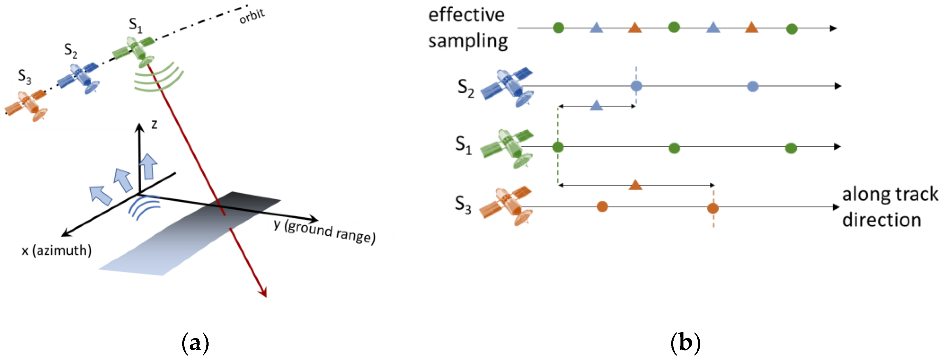
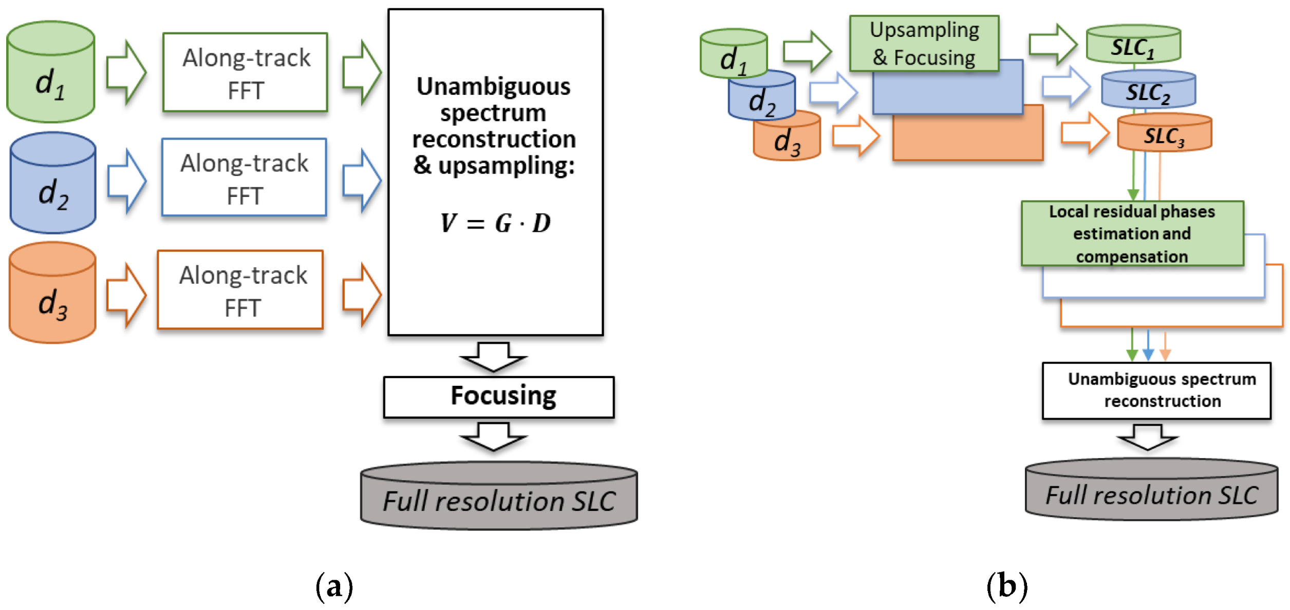
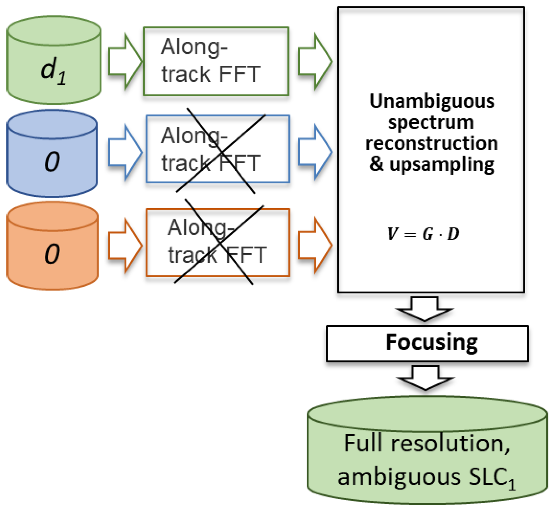
2. Multichannel Processing of Data from Compact SIMO Formation

The usual approach for multichannel recombination is shown in Figure 2a [8,9,23,24]. The set of N range compressed datasets is transformed into the azimuth wavenumber domain ( k x ) and then merged to a wideband spectrum by the following matrix operator, which is applied to each sample in the Doppler spectra:
V = G D V 1 k x V 2 k x + k x s V N k x + N k x s = g 11 g n m g N 1 g N N D 1 k x D N k x
where D is the [N,1] column vector formed by taking one spectral sample for each data set, G is the reconstruction matrix formulated, for example, in [8,9,12], and V is a [N,1] vector with unfolded spectral contributions.
The effect of the multichannel recombination on two-dimensional data spectra is demonstrated in Figure 3. In particular, Figure 3a shows the ideal wideband spectrum of the fine-resolution image to be reconstructed. The undersampling of each acquisition, caused by the low PRF, creates a N-time spectral folding along kx, as shown in Figure 3b. The generation of the full-resolution single look complex image can be split into the following steps:
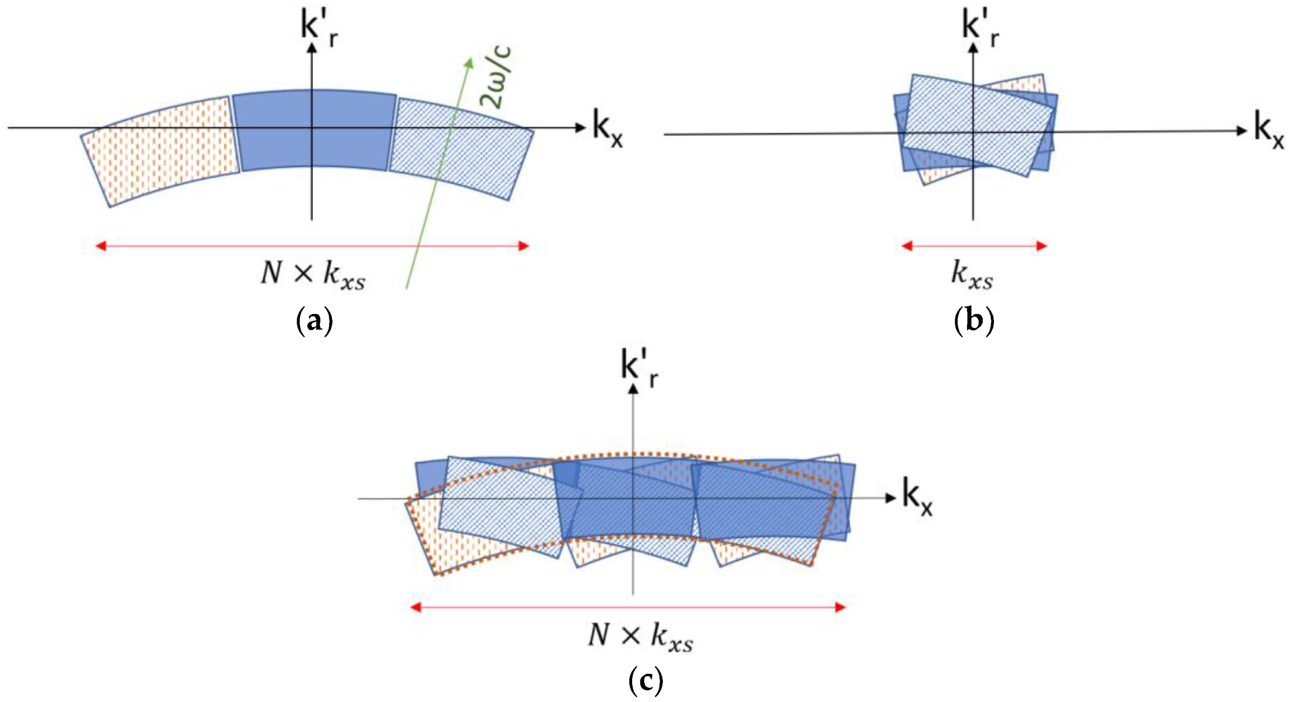
  • The data acquired by the n-th sensor are upsampled by first transforming into the Doppler domain and then replicating (mosaicking) N-times to form the complex spectrum shown in Figure 3c.
  • Each of the N spectral replicas is weighted by the term g n , m (n being the image, and m it the replica) according to (2).
  • All N images are summed together, obtaining a single RGC with a broad Doppler spectrum.
  • The data are focused, obtaining the final fine-resolution ambiguity-free image.
The approach we propose inverts steps 3 and 4 to obtain a set of focused images before compensating for the ambiguities. Loosely speaking, we first focus all the data on the fine grid of Figure 1b, but we do not sum them until residual knowledge errors are estimated and compensated.
The equivalence of the two approaches stems from the linear superposition are suggested in Figure 4 As an example, let us formulate the multichannel recombination (2) by feeding only the first acquisition (and the others being null):
V k x = V 1 k x V 2 k x + k x s V N k x + N k x s = g 11 g n m g N 1 g N N D 1 k x 0 0 = D 1 g 11 D 1 g 21 D 1 g N 1
Equation (3) can be interpreted as a weighted combination of the N-times mosaicked Doppler spectra of the first image, where the weights are the elements g 1 , n k x of the matrix G, represented in Figure 3c. Then, by switching the weighted combination (3) and the focusing kernel, we obtain the alternative procedure of Figure 2a and Figure 4, where data are first oversampled and focused and then recombined as post-processing.

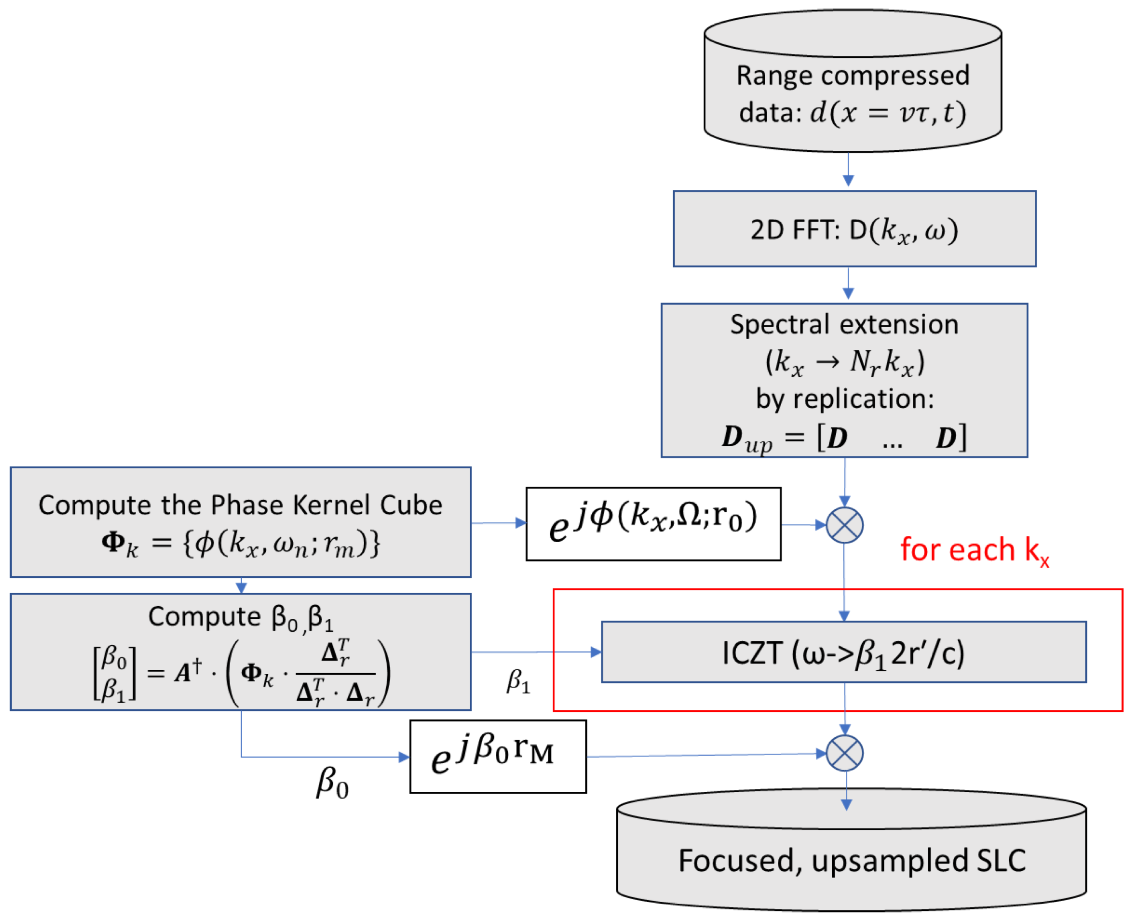
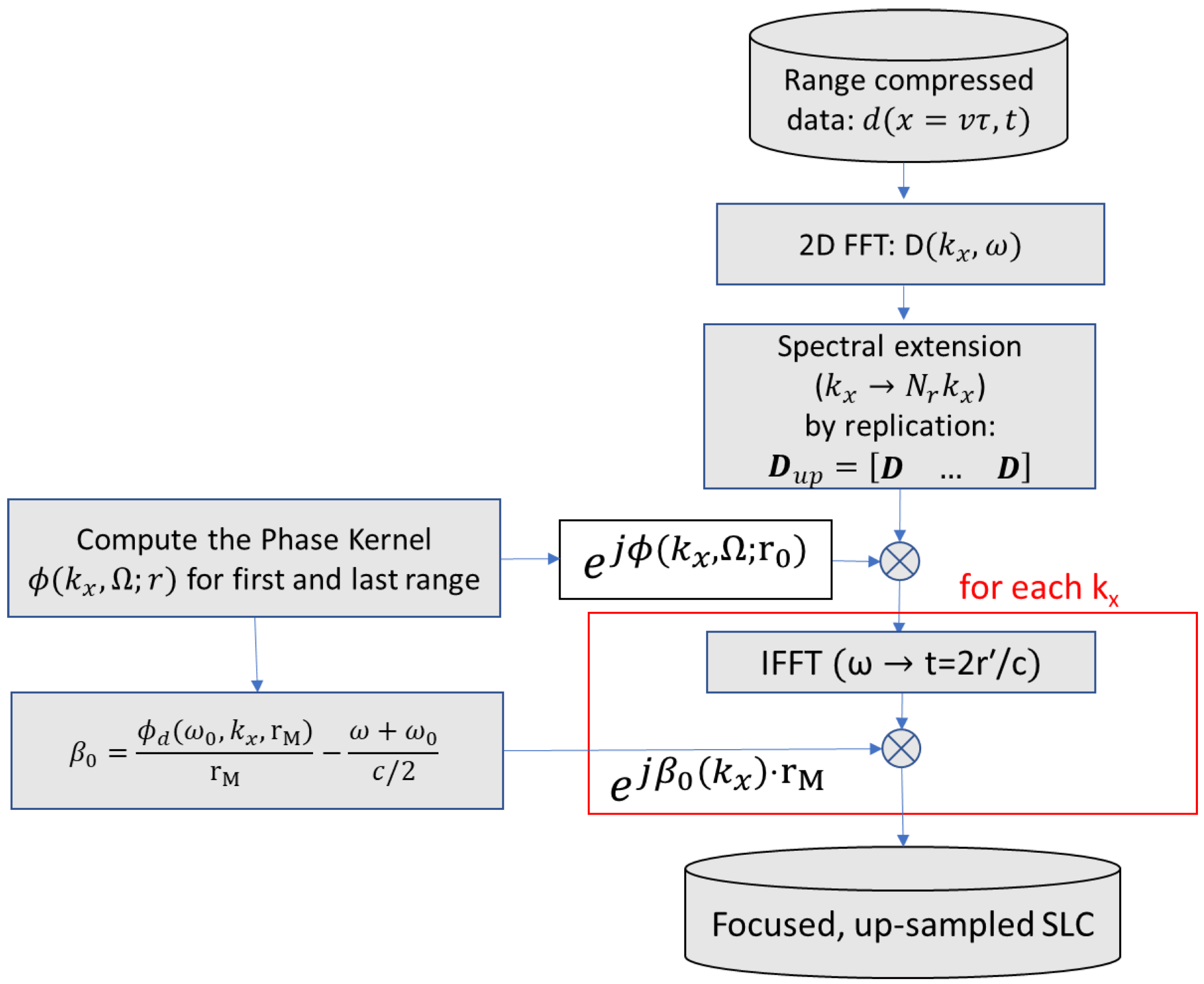
3. Efficient and Flexible Wavenumber Domain Implementation

The objective of the section is to define a numeric wavenumber domain (WD) implementation of the entire procedure in Figure 2b, which adequately copes with the curved orbit.

3.1. Implementation of Curved Orbit Focusing and Upsampling

WD focusing kernels were derived for rectilinear tracks, and their adaptation to the curved orbit case introduces phase errors and biases [16,22,25]. Several alternatives were developed in the literature based on modified, extended chirp-scaling approaches [26,27,28]. However, these approaches are not really needed for the case discussed here, whereas fast and accurate enough kernels can be formulated by numerical methods [19,25,29]. More specifically, let us start from the classical approach for straight orbit derived in Appendix A. The focused scene can be expressed in the azimuth wavenumber and range domain as from (A9):
U k x , r = U c k x , ω exp - j β 0 k x r exp j ω 2 r c β 1 k x d ω U c k x , ω = D k x , ω H c 0 * k x , ω exp - j ω + ω 0 c / 2 t 0
where r 0 is the slant range of the target closest to the sensor, r = r - r 0 is the relative slant range, D k x , ω is the two-dimensional-FT of the RGC data, H c 0 k x , ω is the two-dimensional-FT of the impulse response of a target at a range r 0 , and β 0 , β 1 are two parameters originated by the series expansion of the exact operator (A20).
To generalize (4), the kernel H c 0 should be evaluated numerically for the curved orbit, as shown in Appendix B. One can easily check that doing so (4) would provide the proper focus for those targets located at the closest approach, r 0 , which corresponds to r = 0 .
The role of the parameters β 0 , β 1 is then to extend the depth of focusing to targets at any range r = r - r 0 0 , within some approximation. To find the best values of those parameters, we first evaluate the spectrum of the target at range r , which can be expressed as H c * k x , ω , r = H c 0 exp j ϕ d k x , ω , r , and then we impose the fit:
exp j ϕ d k x , ω , r exp r β 0 k x + β 1 k x 2 ω c .
In particular, two numerical methods are proposed here: the numerical monochromatic (NM) and the numerical chirp-Z transform (NCZ), summarized in Figure 5 and Figure 6. They differ in the fitting accuracy of (5). The fastest method, the NM, imposes β 1 to be unitary, and then implements (4) by an inverse FT. The slowest, but most accurate, (NCZ), accounts for non-unitary β 1 by implementing (4) as an inverse chirp-zeta transform (CZT) at the cost of three fast Fourier transforms (FFT) [30].
The coefficients β 0 k x , β 1 k x are evaluated as the best approximation of (5):
ϕ d ( ω , k x , r ) r β 0 k x + β 1 k x 2 ω c ,
To this aim, we estimate the phase surface numerically ϕ d for M ≥ 2 range bins ( r m ) as described in Appendix B, obtaining, for each kx, a matrix Φ k = { ϕ d ( ω n , r m ; k x ) } of size [N,M]. Then, the vector B = β 0 β 1 T is retrieved by the least square fitting of (6):
Φ k A B Δ r T A = 1 1 4 π f s c N n 1 4 π f s c N - 1 ; B = β 0 k x β 1 k x ; Δ r T = 0 M - 1 d r
where f s is the sampling frequency and d r is the step of the slant-range grid assumed in (6). The solution is:
B = A T A - 1 A T Φ k Δ r T Δ r T Δ r = A Φ k Δ r T m m 2 d r 2
where A is the pseudoinverse of A .
In the NM approach, the procedure simplifies, since we impose β1 = 1. Therefore β 0 is retrieved by fitting (6) near the end of the processing block, r M :
β 0 = ϕ d ω 0 , k x , r M r M - 2 ω + ω 0 c
Notice that, for the straight orbit, the numeric approach defaults to the classical one [16,31,32], as results from (A4) and (9):
β 0 = ω + ω 0 c 2 2 - k x 2 - 2 ω + ω 0 c - k x 2 c 4 ω 0

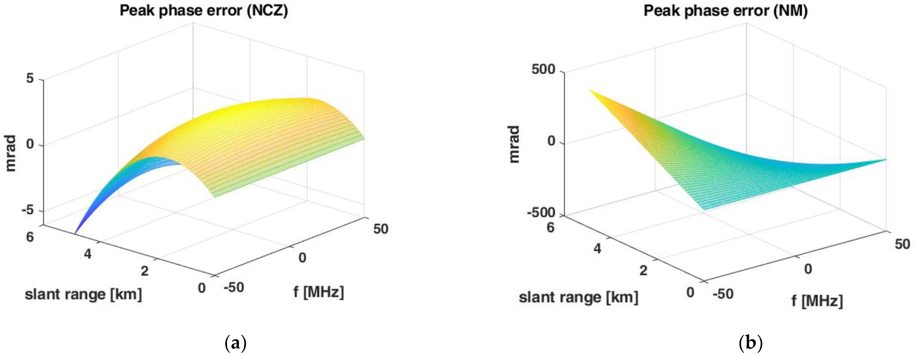
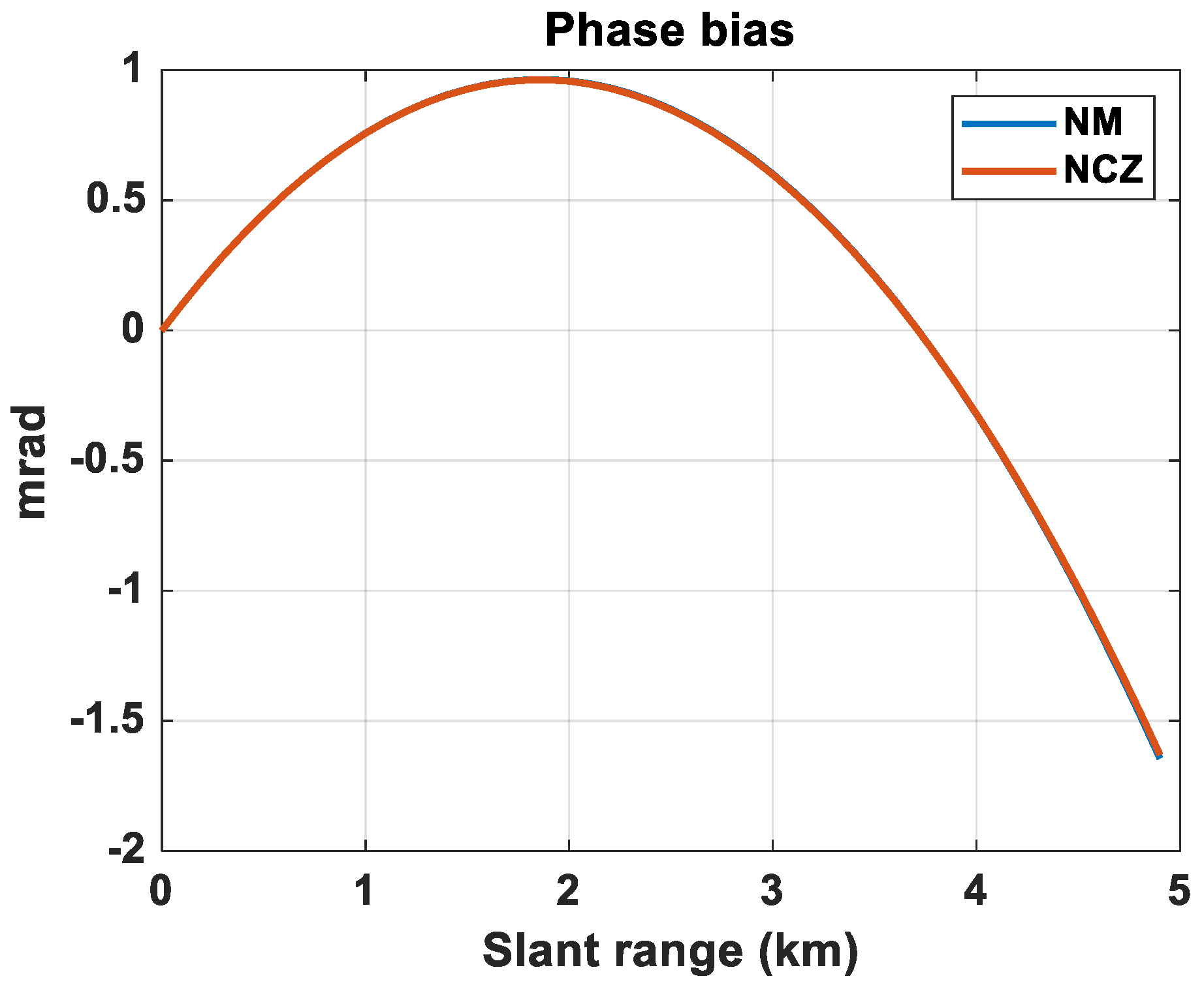
3.2. Phase Preservation

The phase preservation of the focusing approach is evaluated here by considering a typical orbit of a LEO SAR at 500 km altitude. Specifically, we started from a TLE file of Capella Space 4, whose main orbit parameters are listed in Table 2. A set of state vectors (SVs) was generated with the MATLAB aerospace toolbox and used for simulation and focusing. We remind our readers that the interest here is to show the capability of the processor to cope with the orbit curvature.
The phase preservation can be checked by evaluating, for each range, the error in fitting (6):
ϕ e r r r , k x , ω = ϕ d - r β 0 k x + β 1 k x 2 ω + ω 0 c
That phase error, evaluated for kx corresponding to 0.6° squint, has been represented in Figure 7 as a function of frequency and range. We assume a processing block of 5 km in the slant range, which does not introduce any limitation, since it is much larger than the range migration (~8 m). A block-wise implementation is not only needed for quality, but also desired for efficiency and parallelism. NCZ has a negligible peak phase error, less than 5 mrad, whereas, for the NM version, the error is noticeable, but it is less than the acceptable limit of 1 radian [17,32].
Phase bias is even more critical than the peak error since slight values could lead to visible artifacts in the interferometric products [33]. Such bias is one of the major limitations in implementing a processor defined for rectilinear geometries, even for very small blocks, hindering an efficient implementation. The bias can be evaluated by integrating the phase error (11) as a function of range:
ϕ b i a s r = exp ( j ϕ e r r ( r , k x , ω ) ) d k x d ω ,
Results are shown in Figure 8 for the block size of 5 km for both methods. The bias is kept within ~2 mrad in both cases, which fulfills the very stringent conditions of the CEOS offset test [21].

3.3. Multichannel Recombination

The multichannel recombination, discussed in Section 2, requires the knowledge of the inverse matrix G(kx) that can be computed as in [24]:
G ( k x ) = H ( k x ) H * ( k x ) H ( k x ) + k w I N - 1 ,
where I N is the [N,N] identity matrix, and k w is the Wiener parameter that rules the trade-off between ambiguities suppressions and SNR. The [N,N] matrix H is made by pure phase terms, H n m , that implement the correction between the effective bistatic system made by the n-th sensor and the transmitter and the monostatic equivalent used for focusing (A1). For the rectilinear track [8,11,12]:
H n m k x , ω = exp - j ω 0 c x n - x m 2 4 r p exp j x n + x m 2 k x ,
where x n is the along-track position of the n-th receiver, and x m is the transmitter’s position. The first exponential in (14) compensates the bistatic path excess w.r.t the equivalent monostatic sensor positioned at ( x n + x m )/2. For a target located in ( x p , r p ), the path difference amounts to:
Δ R = R b i s S n , S m , P - 2 R m o n o S n + m 2 , P = r p 2 + x - x n - x p 2 + r p 2 + x - x m - x p 2 - 2 r p 2 + x - x n + x m 2 - x p 2
x - x n - x p 2 2 r p + x - x m - x p 2 2 r p - 2 x - x n + x m 2 - x p 2 2 r p = x n - x m 2 4 r p .
This term is a delay that is approximated for a monochromatic system by:
H n m ω = exp - j ω + ω 0 c Δ R exp - j ω 0 c Δ R = exp - j ω 0 c x n - x m 2 4 r p ,
that is consistent with (14). We point out that this term is so slowly varying with range that it can be kept constant for the whole processing block of 5 km (see Section 3.3). It would change the phase term only by a few parts per million, according to the parameters in Table 2, even for a large sensor separation of 1 km.
The second term in (14) is the along-track shift needed to align the focused image to the equivalent monostatic sensor located in ( x m + x n ) / 2 . This shift is not correct for the curved orbit.
The simplest way to adapt the recombination to the actual case is to replace (14) with the residual operator:
H n m k x , ω , r p exp j ω c R n m ω 0 , r p - 2 R m ω 0 , r p exp - j k x x d x ,
where R n m is the bistatic hodograph computed for the n-th sensor and the receiver, assuming a target at mid-range r p , and 2Rm is the monostatic one. The spectrum (18) is computed as described in the Appendix B, but assuming ω=ω0 and approximated to the first order in k x . It is important that all hodographs are computed by assuming the same azimuth, as well as slant range (x,r) reference, which would implicitly compensate for the along-track shifts of the different sensors.

4. Results

The quality of the overall focusing and multichannel reconstruction as post-processing has been tested by simulating a realistic scenario of point and distributed targets acquired by a sensor moving along the 500 km LEO orbit described in Table 2. The parameters of the system and mission are listed in Table 1. We have generated two sets of simulated data:
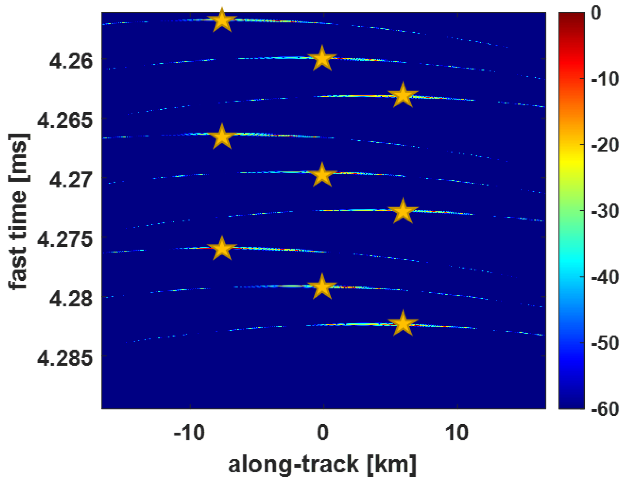
  • a set of nine-point targets, spanning an entire processing block of 5 km in slant range and five footprints in azimuth;
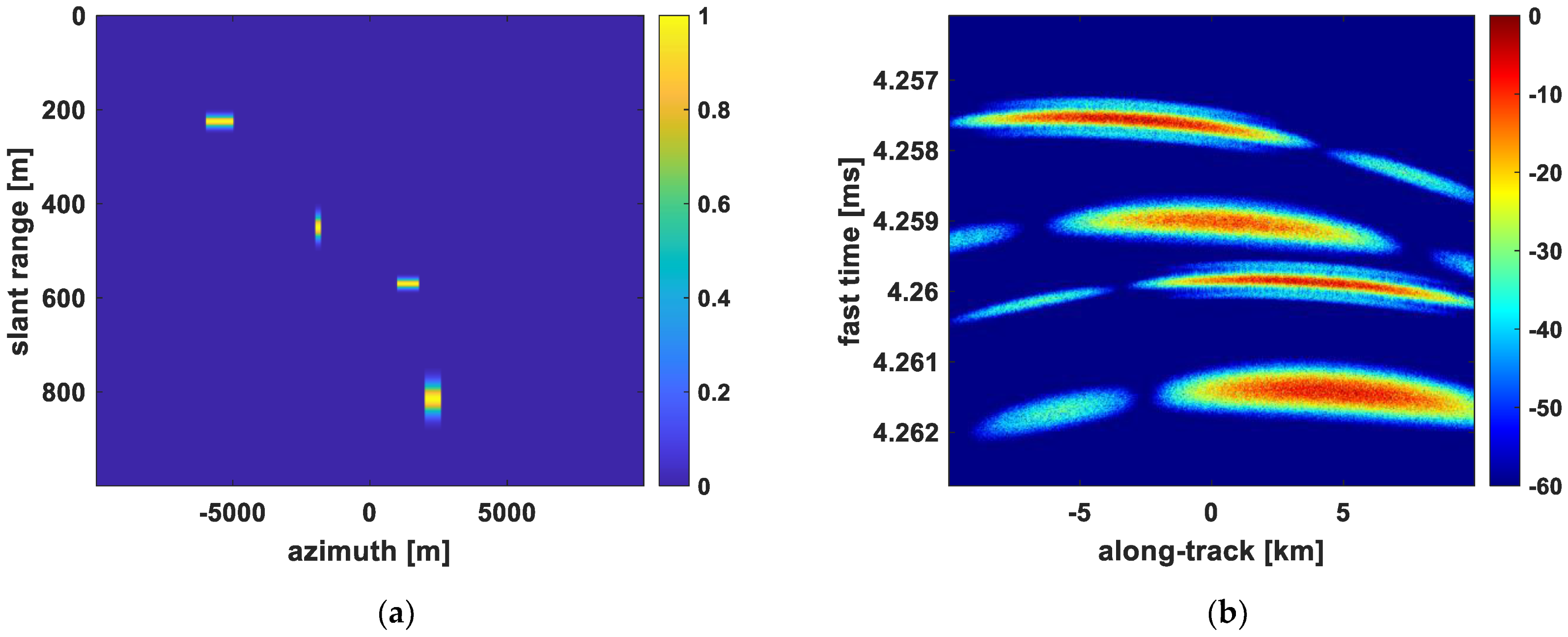
  • a set of distributed targets spanning a block of 1 km in slant range and three footprints in azimuth.
A complex random noise was added to the RGC data in both cases. We have considered a relative sensor distance of about 150 m, with two different configurations:
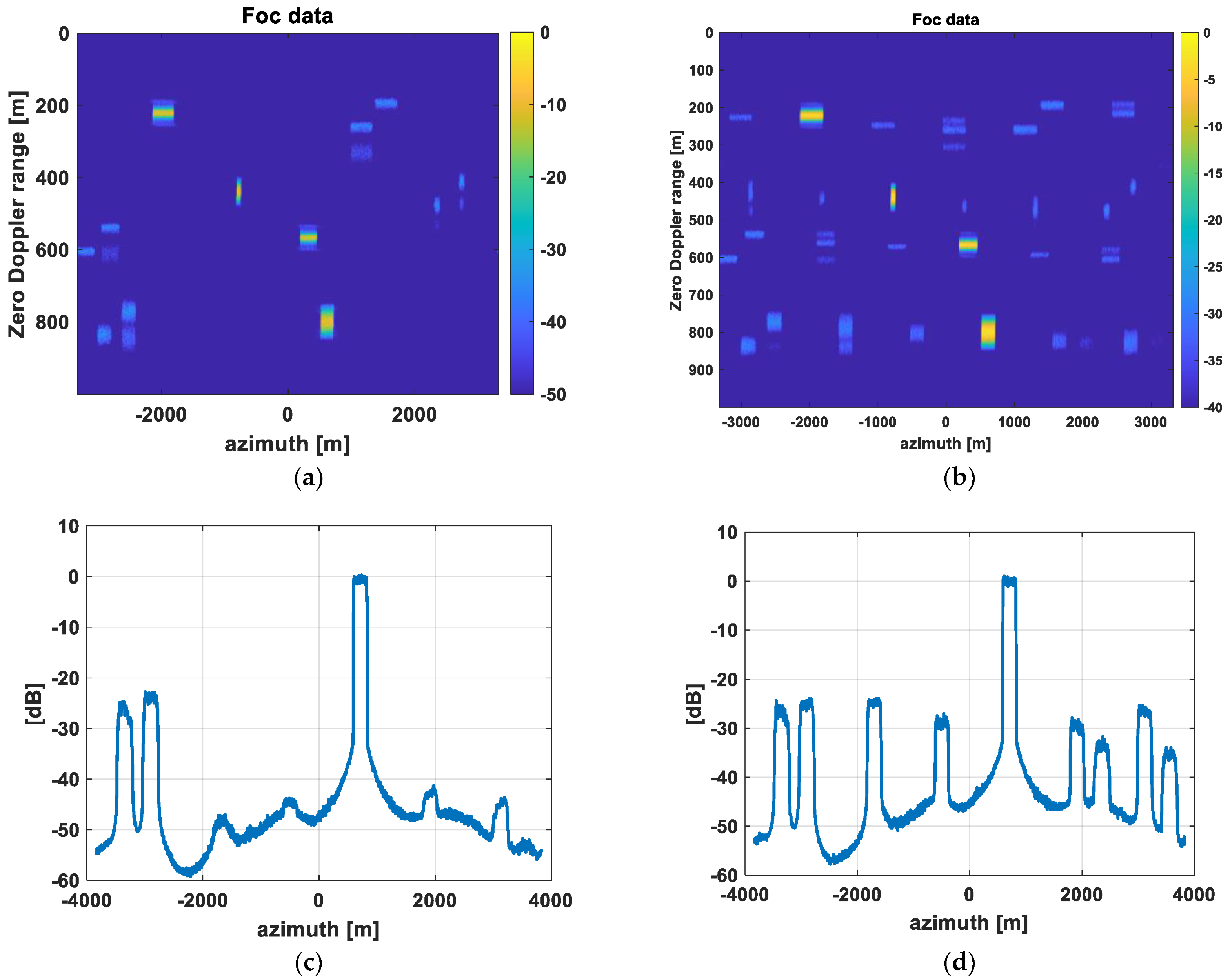
  • the optimal sensor displacements, foreseen by the anti-DPCA condition (1), for which perfect ambiguities-free recombination could be achieved;
  • shifting the second and third sensors, respectively, by 50 cm and −50 cm w.r.t the case above. So doing, the equivalent monostatic phase centers are shifted by ±25 cm, a significant fraction of the fine image resolution La/2 = 1.5 m. This condition stresses the capability of the inversion to remove ambiguities as much as possible.
The matrix inversions (13) have been computed by assuming the Wiener parameter k w = 0.3 . The most efficient NM version was used for focusing, as it did not lead to appreciable artifacts, in concordance with the results of Section 3.3, even considering a squint angle of 0.2° and the largest block of 5 km.

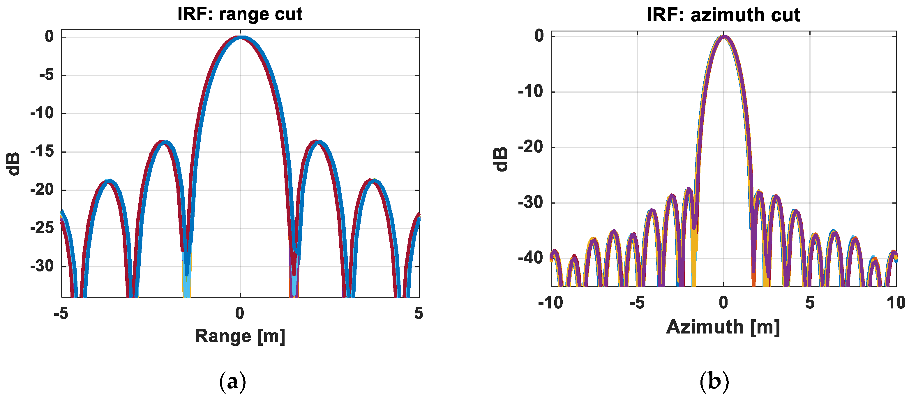
4.1. Point Target Analysis

The set of nine-point targets is represented in Figure 9, which draws the amplitude of one of the N = 3 range-compressed, subsampled images. Stars mark the zero-Doppler position of the targets. After focusing and multichannel recombination, the end-to-end impulse response function along range and azimuth is drawn in Figure 10. A significant oversampling has been applied to assess resolution and sidelobes. However, almost no difference is found in the impulse response functions of all targets, where the nominal slant range and azimuth resolutions of ~1.5 m were measured. The plots of Figure 10 refer to the non-ideal sensor displacements. Still, no difference could be appreciated to the ideal one, similar to the behavior close to the target position.
The suppression of ambiguities by the multichannel combination is evaluated by the energy of the focused impulse response, integrated over range and azimuth, for the target in the middle of the scene in Figure 11. The top panel of Figure 11 refers to the ideal along-track positioning of the sensors, in which only the ambiguities coming from the 3 m SAR antenna are visible. In the bottom panel, the wrong positioning of the two receiving sensors, by 0.5 and −0.5 m w.r.t the optimal case, is considered. The positional error causes 2 × (N − 1) = 4 additional ambiguities. The ambiguities’ energy level is evident but comparable to the one of the fine resolution SAR. Note that the same results are obtained when performing the combination before and after focusing, as seen in Figure 11b,c. This qualifies the whole processing chain and the positioning error.

4.2. Distributed Area Target Analysis

Point target simulation provides all the input to evaluate the end-to-end performance regarding resolution, sidelobes, and ambiguities. However, distributed targets help to analyze ambiguity structures and their suppression. To that aim, we have generated a set of patches of different shapes distributed over the whole image. The map of the simulated distributed scene is provided in Figure 12a, representing the ground truth. The overall scene size is that of a processing block, 1 km × 12 km (slant range, azimuth), where the small area patches result from half a million-point targets overall. The range-compressed, azimuth-defocused data are shown inb, referred to as one of the N = 3 acquisitions. The illumination pattern of the wide-aperture antenna is visible, extending for the entire footprint and at least one sidelobe.
The amplitude of data after focusing and multichannel recombination as post-processing, following the entire chain in Figure 2b, is represented in Figure 13. Multi-looking over local windows of 3 × 3 samples was performed. In the case of perfect spacing (Figure 13a), only the ambiguities due to the 3 m antenna can be seen. The amplitude of such ambiguities w.r.t the target is smaller than −25 dB, which is comparable to the typical values of spaceborne SAR systems, such as Sentinel-1 [34].
In the other case, Figure 13.b also shows the residual ambiguities from the improper multichannel recombination. They are at the same level of those due to the SAR antenna, and therefore they are acceptable in a SAR mission.

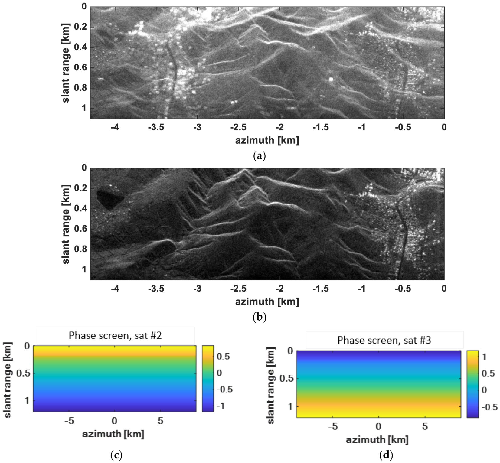
4.3. A Realistic Scenario: The Impact of Across-Track Baselines

So far, we have assumed the same track for all the sensors in a fixed Earth reference. Yet, even the best design and control of the formation flying would leave some residual offset between sensor tracks, as shown, for example, in [35,36,37]. We then assumed that the tracks of the second and the third satellites are displaced respectively by 1 m and −1 m in the direction perpendicular to the line-of-sight, w.r.t the track of the first sensor. For simplicity, we keep this offset constant within a few synthetic apertures, lasting a couple of seconds.
The across-track baseline results in an unwanted multiplicative phase screen, different for each channel, which interferes with the correct multichannel recombination and prevents suppression of ambiguities. The proper compensation of this effect is quite complicated, and it is indeed one of the major objectives of the present literature [12,38,39]. However, for small baseline and smooth topography, first-order mitigation could be performed as suggested in [6,39,40], which consists in estimating the residual phase screen, given the precise knowledge baselines and the elevation of the scene’s center, and removing it prior to the multichannel recombination.
We simulated the compensation of the across-track baseline in two scenarios. First, the conventional method was employed, as described in Figure 2a. Since the phase screen was essentially along the range, the compensation task can be performed on the range compressed images. However, the specific orbit knowledge for near real-time applications is limited to several centimeters [41]. We assumed a 1 cm error in the knowledge of both normal and perpendicular directions. Such lack of precision affects the accuracy of the computation of the phase screens and then hinders the quality of the multichannel combined image. The result of the conventional processing is shown in Figure 14a: the quality is compromised by the uncompensated ambiguities, which spread throughout the image.
The figure was generated by simulating a set of N = 3 multichannel data. A complex reflectivity map, obtained by multi-temporal averaging over 80 COSMO-SkyMed images, was used with a DEM and sensor’s orbit to simulate the source RGC data.
The procedure in Figure 2b was implemented by upsampling and focusing separately on the three datasets. This allowed for a fine, data-driven baseline estimation with a sub-millimetric accuracy, as from [42,43,44]. The refined baselines are then used to compute the precise topographic phase screens shown in Figure 14c,d. The phase variation is tiny, yet its compensations lead to the final-multichannel image, shown in Figure 14b, which is almost free from ambiguity clutter.

4.4. Efficiency

The proposed approach, which first upsamples and then merges the N ambiguous focused images, is clearly less efficient than the classical merge and upsample procedure. To assess performance, a set of prototype Matlab codes for the different methods has been profiled and optimized to evaluate and compare their efficiency. In particular, we have considered the numerical monochromatic and the numerical chirp-Z approaches and measured the computing time on a modern eight-core desktop PC. The time reported in Table 3 refers to focusing one range compressed data block as in Figure 9, approximately 5000 × 9400 samples. The cost of the “multichannel recombination” in the bottom left of the table has been estimated by assuming the recombination as a fast convolution implemented in ten blocks along the azimuth. Notice that the recombination is essentially a fractional resampling, as from (14), requiring a very short operator in the along-track space. In the most favorable case, where condition (1) is perfectly met, one could interleave the focused data at no cost.
From the table, one notices that the conventional approach, on the right column, is the most efficient, where the NM method is approximately 2.5 times faster than the NCZT one. However, if we implement the proposed approach, where the images are up-sampled and focused on-the-fly, by each sensor, then the overall computing time is half of the usual approach.

5. Conclusions

A new processing framework has been proposed, suited for compact SAR formations where acquisitions from different sensors are combined into a unique full-resolution image, such as SIMO or MIMO SAR. The processing scheme is based on oversampling and focusing on each acquisition, while leaving the multichannel reconstruction as the last step. This procedure is useful to integrate the estimation and compensation of impairments acting on a local space-varying scale, similar to the effect of topographic phases.
A very efficient, full numerical implementation of monostatic focusing and multichannel recombination has been discussed. The result is a phase-preserving processor whose efficiency is compared to a couple of bidimensional FT. The scheme has been validated with point and simulated targets generated by assuming the orbit of a typical LEO SAR flying at 500 km altitude. The method has been shown effective for the mitigation of ambiguities due to unknown across-track baselines between sensors by simulating a realistic SAR scene, starting from X-band Cosmo-SkyMed data.

Author Contributions

Conceptualization and project administration, A.M.G.; methodology, software, investigation and data curation, N.P.; writing, A.M.G. and N.P.; formal analysis, S.T.; validation, M.M.; supervision, C.P. and A.M.G. All authors have read and agreed to the published version of the manuscript.

Funding

This research received no external funding.

Institutional Review Board Statement

Not applicable.

Data Availability Statement

No dataset is publicly available.

Acknowledgments

COSMO-SkyMed data, used for simulating the X-band reflectivity, were provided within the ASI (Agenzia Spaziale Italiana) open call for science.

Conflicts of Interest

The authors declare no conflict of interest.

Appendix A. Derivation of Focusing Kernels for Curved Orbit

WD focusing has been used for over three decades for its efficiency and quality, and it is the one usually assumed for SIMO formations. Here, we start from the basics of SAR focusing on deriving two efficient approximations suited for the curved orbit of an LEO sensor. The focused image in the azimuth, as well as slant range domain, u(x,r), are obtained by the convolution along azimuth of the range compressed data d(x,t) with the matched phase kernel [32]:
u x , r = d x , t - t 0 x h * x , t - 2 r c ; r d t ,
where t0 is the time for the first raw sample, according to the geometry sketched in Figure A1, x stands for correlation along azimuth, h*( ) is the focusing kernel, phase-matched to the impulse response of a target located in (x,r). Factor two in the argument of h*, the two-way range of the monostatic SAR, is here addressed.
Figure A1. Representation of the geometry of the LEO SAR acquisition in the curved orbit case (left), and for the raw data (right). The orbit curvature has been exaggerated.
Remotesensing 15 01644 g0a1
To derive the WD scheme, we transform both members of (A1) from x to kx, and we use Parseval identity to evaluate the time domain integral [16]:
U k x , r = D k x , ω H * k x , ω ; r exp - j ω + ω 0 c / 2 t 0 d ω .
We are not interested in evaluating the focused data from the origin, r = 0, but rather from a minimum slant range, r0, as shown in Figure A1. Then, the focused field to be estimated is U 0 :
U 0 r = U r + r 0 = D k x , ω H * k x , ω ; r + r 0 exp - j ω + ω 0 c / 2 t 0 d ω ,
where r’ = r − r0 is the actual range axis of the focused image.
In the case of a straight orbit, the kernel H is the filed propagation operator [16]:
H * k x , ω , r = exp j r ω + ω 0 c / 2 2 - k x 2
That can be plugged into (A3), giving:
U 0 r = U r + r 0 = D k x , ω H * k x , ω ; r 0 H * k x , ω ; r exp - j ω + ω 0 c / 2 t 0 d ω
For small squint angles, as usually is for LEO SAR, the kernel H*(…) can be approximated to the first power of ω:
U k x , r = Φ 0 r , k x U 0 k x , ω exp j r 1 4 k x 2 c ω 0 2 ω exp - j ω 2 r c d ω U 0 k x , ω = D k x , ω H * k x , ω , r 0 exp - j ω + ω 0 c / 2 t 0 Φ 0 r , k x = exp - j r k x 2 c 4 ω 0 + 2 ω 0 c
Equation (A6) is the one that drives the efficient implementation of many WD processors [16,31,32,32,45,46,47]: the two-dimensional transform of the data is first multiplied by the matched phase reference H * k x , ω , r 0 , resulting in the term U 0 k x , ω . Thereafter we can identify two different approaches.
The first one results from ignoring the first exponential within the integral (A6) in favor of the second:
1 4 k x 2 c ω 0 2 2 c ω 2 ω 0 2 sin 2 ψ 2 1
Then, (A6) becomes an inverse FT from ω to t = 2r’/c:
U k x , r = Φ 0 r , k x F - 1 U 0 k x , ω t = 2 r c
This method is known as the monochromatic ωk [16,31,32]. We observe that approximation (A7) is well acceptable in the X-band, since both the antenna aperture and the fractional bandwidth, Δω/ω0, are pretty small.
The second approach is a straight implementation of (A6) with no approximation, which would be suited for wide antenna aperture and/or large fractional bandwidths, similar to the case for L-band systems. The implementation relies in on the use of the chirp-Z transform [30,46]. We need to rewrite (A6) as follows:
U k x , r = Φ 0 r , k x U 0 k x , ω exp - j ω 2 r c 1 + α d ω α = 1 8 k x 2 c 2 ω 0 2 1
To acknowledge in (A9) an inverse CZT, a Fourier transform is computed in the linearly-scaled time axis. The method, conceptually equivalent to the chirp scaling approach [18], is more time-consuming, as it requires three FTs instead of one, which is the case for the monochromatic case.

Appendix B. Numerical Implementation of the WD Kernel

We detail here the numerical implementation of the phase-matched WD focusing operator, evaluated for an impulsive target P located in the slant range r. We assume the acquisition monostatic, where the sensor moves along a curved path, defined by the state vector S(τ) = {Sx(τ), Sy(τ), Sz(τ)}, τ being the slow time reference. The SAR acquisition is then modeled by the impulse response:
h τ , r = p t - R 2 m c exp - j 2 ω 0 R 2 m c ,
where p(t) is the range compressed pulse (that we assume here ideal with constant power spectrum), t is the fast time, and R is the hodograph, the two-way sensor-target distance:
R 2 m τ ; r = 2 S τ - P r .
We assume the reference slant range, azimuth plane directed along the mean satellite velocity along-track, where azimuth axis is x = vsτ. We remind our readers that SAR focusing is accomplished by correlation with a kernel that is phase-matched to the impulse response (A10). Its two-dimensional Fourier transform (FT) is [32]:
H g ω , k x ; r = e x p j Ω R 2 m exp j k x x d x where   Ω = ω + ω 0 c
The expression for hyperbolic hodograph for the straight orbit is in (A4). In the generalized case of a curved orbit, we can evaluate H g by the numerical implementation of the method of stationary phase [19,25,29,48]. According to this method, the FT in (A12) is approximated as follows:
H g ω , k x ; r e x p j Ω R 2 m τ f + k x v s τ f ,
where τf are the stationary phase times, those nulling the derivative of the phase:
Ω R 2 m τ | τ = τ f + k x v s = 0 R 2 m τ | τ = τ f = - k x Ω v s ,
For the numerical computation of the two-dimensional spectrum Hg, we define a uniform grid spanning the support in (kx, Ω):
4 π c f 0 - B 2 Ω 4 π c f 0 + B 2 4 π f d c v s - f p r f 2 v s k x 4 π f d c v s + f p r f 2 v s
where fdc is the Doppler centroid. We compute the value of the parameter:
ξ = - k x Ω
for each point in the (kx, Ω) grid. Given ξ, we compute the stationary time, tf, as the solution of:
R 2 m τ | τ = τ f = ξ v s .
This stationary time is then plugged into (A13) to compute the kernel spectrum H g ω , k x .
A very effective method to solve (A14) is the one proposed in [29]. We first compute a polynomial approximation for the two-way hodograph (A11): a fourth-order one is well enough for our case:
R 2 m x = v s τ f = a 0 + a 1 τ f + a 2 τ f 2 + a 3 τ f 3 + a 4 τ f 4 ,
then we derive it according to (A14):
ξ = 1 v s R 2 m τ = 1 v s a 1 + 2 a 2 τ + 3 a 3 τ 2 + 4 a 4 τ 3 ,
that we may rewrite as:
ξ - b 0 = b 1 τ + b 2 τ 2 + b 3 τ 3 w h e r e b n = a n v s ,
The solution of (A14) needs to compute τf, given ξ, which is accomplished by computing the reverse polynomial series [49]:
ξ f = d 1 ξ - b 0 + d 2 ξ - b 0 2 + d 3 ξ - b 0 3 w h e r e d 1 = b 1 - 1 d 2 = - b 1 - 3 b 2 d 3 = b 1 - 5 2 b 2 2 - b 1 b 3 ,
The method is summarized in the flowchart of Figure A2a, implemented by the following steps:
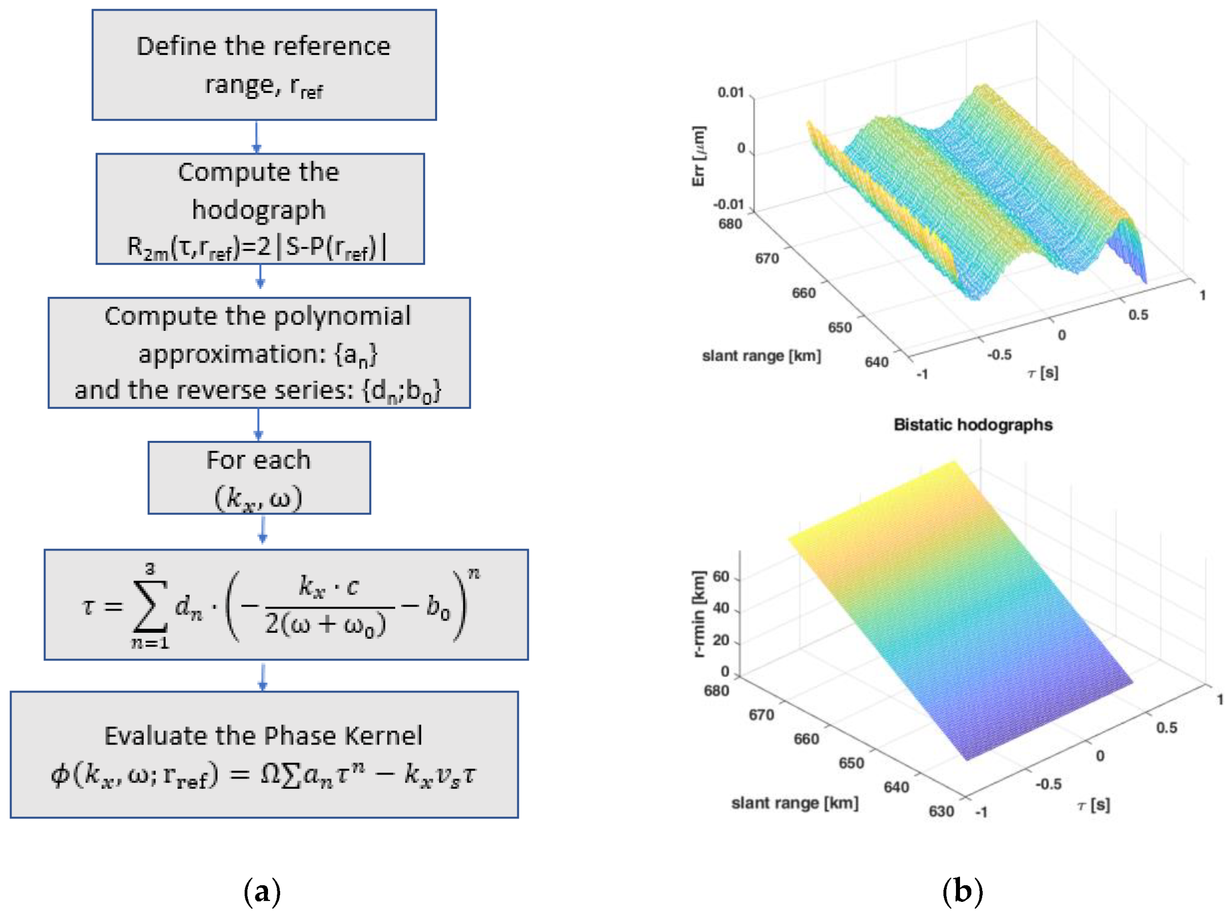
  • Compute the two-way hodograph that is double the Euclidean distance between the sensor (all along its orbit) and the target at slant range, r, according to (A10). Note that if this distance is smooth, then a few samples need to be evaluated.
  • Fit a fourth-order polynomial deriving the coefficients { a 0 a 4 } in (A19);
  • Derive the polynomial coefficients { b 0 b 3 } and then { d 1 d 3 } as from (A20) and (A21);
  • Evaluate the spectra H g ω , k x for each wavenumber pair, (kx,Ω), by computing first ξ from (A16), then τ f = τ ξ from (A19), and finally R from (A18).
This last step is quite efficient, as it involves only polynomial evaluations. However, its impact on the overall computational complexity of the overall processing is still significant. We find out that, when performance is mandatory, some improvement in speed with no significant degradation in quality is achieved by evaluating the polynomials on a subsampled grid in the ω domain and then linearly interpolating them for all the samples.
So far, we have assumed the monostatic case. It is, however, straightforward to extend the method to a bistatic system just by replacing (A11) with the actual bistatic hodograph in:
R b i s τ ; r = S T τ - P r + S R τ - P r ,
where ST and SR are the positions of the transmitter and the receiver. To evaluate the suitability of the 4th-order polynomial approximation, we have computed a set of bistatic hodographs by assuming the curved orbit described in Table 2, spanning the range of about 20 km and synthetic aperture for about 1.6 s. The hodographs and their error with respect to the polynomial interpolation have been plotted in b The error is a tiny fraction of the wavelength.
Figure A2. (a) Flow chart for the numerical evaluation of the two-dimensional spectrum of the matched phase reference. (b) Example of a set of bistatic hodographs (top), computed at different slant range, by assuming the mission parameters and (bottom) the error due to fitting a fourth-order polynomial.
Remotesensing 15 01644 g0a2

References

  1. Villano, M.; Márquez-Martínez, J.; Moller, D.; Younis, M. Overview of Newspace Synthetic Aperture Radar Instrument Activities. In Proceedings of the IGARSS 2022-2022 IEEE International Geoscience and Remote Sensing Symposium, Kuala Lumpur, Malaysia, 17–22 July 2022; pp. 4130–4132. [Google Scholar]
  2. Freeman, A.; Johnson, W.T.K.; Huneycutt, B.; Jordan, R.L.; Hensley, S.; Siqueira, P.; Curlander, J. The “Myth” of the Minimum SAR Antenna Area Constraint. IEEE Trans. Geosci. Remote Sens. 2000, 38, 320–324. [Google Scholar] [CrossRef] [Green Version]
  3. Aguttes, J.P. The SAR Train Concept: Required Antenna Area Distributed over N Smaller Satellites, Increase of Performance by N. In Proceedings of the IGARSS 2003. 2003 IEEE International Geoscience and Remote Sensing Symposium. Proceedings (IEEE Cat. No.03CH37477), Toulouse, France, 21–25 July 2003; Volume 1, pp. 542–544. [Google Scholar]
  4. Gigantino, A.; Graziano, M.D.; Renga, A.; Moccia, A. Simulation of Distributed SAR Images by Multi-Platform Image Syn-Thesis: Application to a CubeSats Formation. In Proceedings of the EUSAR 2022; 14th European Conference on Synthetic Aperture Radar, Leipzig, Germany, 25–27 July 2022; pp. 1–6. [Google Scholar]
  5. Angelone, C.V.; Mancini, M.L.; Tampellini, L.; Maioli, G.; Montano, D.; Giudici, P.; Guccione, F.; Gerace, P.; Gabellini, S.; Falzini, A.; et al. SATURN—A Synthetic Aperture Radar CubeSats Swarm Mission for Earth Observation. In Proceedings of the 73rd International Astronautical Congress (IAC), Paris, France, 18–22 September 2022; pp. 1–11. [Google Scholar]
  6. Aguttes, J.P. The SAR Train Concept: An along-Track Formation of Sar Satellites for Diluting the Antenna Area over N Smaller Satellites, While Increasing Performance by N. Acta Astronaut. 2005, 57, 197–204. [Google Scholar] [CrossRef]
  7. Cerutti-Maori, D.; Sikaneta, I.; Klare, J.; Gierull, C.H. MIMO SAR Processing for Multichannel High-Resolution Wide-Swath Radars. IEEE Trans. Geosci. Remote Sens. 2014, 52, 5034–5055. [Google Scholar] [CrossRef]
  8. Krieger, G.; Gebert, N.; Moreira, A. Unambiguous SAR Signal Reconstruction from Nonuniform Displaced Phase Center Sampling. IEEE Geosci. Remote Sens. Lett. 2004, 1, 260–264. [Google Scholar] [CrossRef] [Green Version]
  9. Cheng, P.; Wan, J.; Xin, Q.; Wang, Z.; He, M.; Nian, Y. An Improved Azimuth Reconstruction Method for Multichannel SAR Using Vandermonde Matrix. IEEE Geosci. Remote Sens. Lett. 2017, 14, 67–71. [Google Scholar] [CrossRef]
  10. Giudici, D.; Guarnieri, A.M.; Guccione, P.; Mapelli, D.; Persico, A. Formation of MIMO SAR Mini-Satellites: Performance Prediction. In Proceedings of the 2021 IEEE International Geoscience and Remote Sensing Symposium IGARSS, Brussels, Belgium, 1–16 July 2021; pp. 1094–1097. [Google Scholar]
  11. Gebert, N.; Krieger, G.; Moreira, A. Multichannel Azimuth Processing in ScanSAR and TOPS Mode Operation. IEEE Trans. Geosci. Remote Sens. 2010, 48, 2994–3008. [Google Scholar] [CrossRef] [Green Version]
  12. Guccione, P.; Monti Guarnieri, A.; Rocca, F.; Giudici, D.; Gebert, N. Along-Track Multistatic Synthetic Aperture Radar Formations of Minisatellites. Remote Sens. 2020, 12, 124. [Google Scholar] [CrossRef] [Green Version]
  13. Cerutti-Maori, D.; Ender, J. Performance Analysis of Multistatic Configurations for Spaceborne GMTI Based on the Auxiliary Beam Approach. IEE Proc.-Radar Sonar Navig. 2006, 153, 96–103. [Google Scholar] [CrossRef]
  14. Krieger, G.; Moreira, A. Multistatic Sar Satellite Formations: Potentials and Challenges. In Proceedings of the 2005 IEEE International Geoscience and Remote Sensing Symposium, 2005. IGARSS ’05, Seoul, Republic of Korea, 29 July 2005; Volume 4, pp. 2680–2684. [Google Scholar]
  15. Giudici, D.; Guccione, P.; Mapelli, D.; Marini, J.; Guarnieri, A.M. RAINBOW-SAR: Enhanced Observation Capability by Multiple Frequency Radar. In Proceedings of the 7th Workshop on RF and Microwave Systems, 10 May 2022. Instruments & Sub-systems + 5th Ka-band Workshop. [Google Scholar]
  16. Cafforio, C.; Prati, C.; Rocca, F. SAR Data Focusing Using Seismic Migration Techniques. IEEE Trans. Aerosp. Electron. Syst. 1991, 27, 194–207. [Google Scholar] [CrossRef]
  17. Curlander, J.C.; McDonough, R.N. Synthetic Aperture Radar; Wiley: New York, NY, USA, 1991; Volume 11. [Google Scholar]
  18. Cumming, I.G.; Wong, F.H. Digital Processing of Synthetic Aperture Radar Data. Artech House 2005, 1, 108–110. [Google Scholar]
  19. D'Aria, D.; Guarnieri, A.M. High-Resolution Spaceborne SAR Focusing by SVD-Stolt. IEEE Geosci. Remote Sens. Lett. 2007, 4, 639–643. [Google Scholar] [CrossRef]
  20. Prats-Iraola, P.; Rodriguez-Cassola, M.; Zan, F.D.; Lopez-Dekker, P.; Scheiber, R.; Reigber, A. Efficient Fourier-Based Evaluation of SAR Focusing Kernels. In Proceedings of the EUSAR 2014; 10th European Conference on Synthetic Aperture Radar, Berlin, Germany, 3–5 June 2014; pp. 1–4. [Google Scholar]
  21. Belotti, M.; D’Aria, D.; Guccione, P.; Miranda, N.; Monti Guarnieri, A.; Rosich, B. Requirements and Tests for Phase Preservation in a SAR Processor. IEEE Trans. Geosci. Remote Sens. 2014, 52, 2788–2798. [Google Scholar] [CrossRef]
  22. Bamler, R.; Schaettler, B. Phase-Preservation in SAR Processing: Definition, Requirements and Tests. DLR Tech. Note Ver. 1995, 1. [Google Scholar]
  23. Gebert, N.; Krieger, G.; Moreira, A. Digital Beamforming on Receive: Techniques and Optimization Strategies for High-Resolution Wide-Swath SAR Imaging. IEEE Trans. Aerosp. Electron. Syst. 2009, 45, 564–592. [Google Scholar] [CrossRef] [Green Version]
  24. Giudici, D.; Guccione, P.; Manzoni, M.; Guarnieri, A.M.; Rocca, F. Compact and Free-Floating Satellite MIMO SAR Formations. IEEE Trans. Geosci. Remote Sens. 2021, 60, 1–12. [Google Scholar] [CrossRef]
  25. Bamler, R.; Meyer, F.; Liebhart, W. Processing of Bistatic SAR Data From Quasi-Stationary Configurations. Geosci. Remote Sens. IEEE Trans. On 2007, 45, 3350–3358. [Google Scholar] [CrossRef]
  26. Moreira, A.; Mittermayer, J.; Scheiber, R. Extended Chirp Scaling Algorithm for Air- and Spaceborne SAR Data Processing in Stripmap and ScanSAR Imaging Modes. IEEE Trans. Geosci. Remote Sens. 1996, 34, 1123–1136. [Google Scholar] [CrossRef]
  27. Wong, F.H.; Cumming, I.G.; Neo, Y.L. Focusing Bistatic SAR Data Using the Nonlinear Chirp Scaling Algorithm. IEEE Trans. Geosci. Remote Sens. 2008, 46, 2493–2505. [Google Scholar] [CrossRef] [Green Version]
  28. An, D.; Huang, X.; Jin, T.; Zhou, Z. Extended Nonlinear Chirp Scaling Algorithm for High-Resolution Highly Squint SAR Data Focusing. IEEE Trans. Geosci. Remote Sens. 2012, 50, 3595–3609. [Google Scholar] [CrossRef]
  29. Neo, Y.L.; Wong, F.; Cumming, I.G. A Two-Dimensional Spectrum for Bistatic SAR Processing Using Series Reversion. GRSL 2007, 4, 93–97. [Google Scholar] [CrossRef] [Green Version]
  30. Rabiner, L.R.; Gold, B. Theory and Application of Digital Signal Processing; Englewood Cliffs Prentice-Hall: Hoboken, NJ, USA, 1975. [Google Scholar]
  31. Wiehle, S.; Mandapati, S.; Günzel, D.; Breit, H.; Balss, U. Synthetic Aperture Radar Image Formation and Processing on an MPSoC. IEEE Trans. Geosci. Remote Sens. 2022, 60, 1–14. [Google Scholar] [CrossRef]
  32. Bamler, R. A Comparison of Range-Doppler and Wave-Number Domain SAR Focusing Algorithms. TGARS 1992, 30, 706–713. [Google Scholar]
  33. Prats-Iraola, P.; Rodriguez-Cassola, M.; De Zan, F.; López-Dekker, P.; Scheiber, R.; Reigber, A. Efficient Evaluation of Fourier-Based SAR Focusing Kernels. IEEE Geosci. Remote Sens. Lett. 2014, 11, 1489–1493. [Google Scholar] [CrossRef] [Green Version]
  34. Sentinel, G. Team, GMES Sentinel-1 System Requirements Document; Technical Report S1-RS-ESA-SY-0001; ESA: Paris, France, 2006. [Google Scholar]
  35. Graziano, M.D.; Renga, A.; Grasso, M.; Moccia, A. PRF Selection in Formation-Flying SAR: Experimental Verification on Sentinel-1 Monostatic Repeat-Pass Data. Remote Sens. 2019, 12, 29. [Google Scholar] [CrossRef] [Green Version]
  36. Graziano, M.D.; Renga, A.; Grasso, M.; Moccia, A. Error Sources and Sensitivity Analysis in Formation Flying Synthetic Aperture Radar. Acta Astronaut. 2022, 192, 97–112. [Google Scholar] [CrossRef]
  37. Kraus, T.; Krieger, G.; Bachmann, M.; Moreira, A. Spaceborne Demonstration of Distributed SAR Imaging With TerraSAR-X and TanDEM-X. IEEE Geosci. Remote Sens. Lett. 2019, 16, 1731–1735. [Google Scholar] [CrossRef] [Green Version]
  38. Kraus, T.; Krieger, G.; Bachmann, M.; Moreira, A. Addressing the Terrain Topography in Distributed SAR Imaging. In Proceedings of the 2019 International Radar Conference (RADAR), Toulon, France, 23–27 September 2019; pp. 1–5. [Google Scholar]
  39. Dogan, O.; Uysal, F.; Dekker, P.L. Unambiguous Recovery of Multistatic SAR Data for Nonzero Cross Track Baseline Case. IEEE Geosci. Remote Sens. Lett. 2022, 19, 1–5. [Google Scholar] [CrossRef]
  40. Lin, H.; Deng, Y.; Zhang, H.; Liang, D.; Jia, X. An Imaging Method for Spaceborne Cooperative Multistatic SAR Formations With Nonzero Cross-Track Baselines. IEEE J. Sel. Top. Appl. Earth Obs. Remote Sens. 2022, 15, 8541–8551. [Google Scholar] [CrossRef]
  41. Wermuth, M.; Hauschild, A.; Montenbruck, O.; Jäggi, A. TerraSAR-X Rapid and Precise Orbit Determination. In Proceedings of the 21st International Symposium on Space Flight Dynamics, Toulouse, France, 28 September–2 October 2009. [Google Scholar]
  42. Bamler, R.; Hartl, P. Synthetic Aperture Radar Interferometry. Inverse Probl. 1998, 14, 4. [Google Scholar] [CrossRef]
  43. Ferretti, A.; Monti Guarnieri, A.; Prati, C.; Rocca, F.; Massonnet, D. InSAR Principles: Guidelines for SAR Interferometry Processing and Interpretation; ESA TM-19 Feb 2007; ESA: Paris, France, 2007. [Google Scholar]
  44. Manzoni, M.; Monti-Guarnieri, A.V.; Realini, E.; Venuti, G. Joint Exploitation of SAR and GNSS for Atmospheric Phase Screens Retrieval Aimed at Numerical Weather Prediction Model Ingestion. Remote Sens. 2020, 12, 654. [Google Scholar] [CrossRef] [Green Version]
  45. Yang, T.; Xu, Q.; Meng, F.; Zhang, S. Distributed Real-Time Image Processing of Formation Flying SAR Based on Embedded GPUs. IEEE J. Sel. Top. Appl. Earth Obs. Remote Sens. 2022, 15, 6495–6505. [Google Scholar] [CrossRef]
  46. Lanari, R. A New Method for the Compensation of the SAR Range Cell Migration Based on the Chirp Z-Transform. IEEE Trans. Geosci. Remote Sens. 1995, 33, 1296–1299. [Google Scholar] [CrossRef]
  47. Ran, J.; Li, X. An Analytical Imaging Algorithm for Parallel Invariant SAR. In Proceedings of the 2018 IEEE 3rd International Conference on Signal and Image Processing (ICSIP), Shenzhen, China, 13–15 July 2018; pp. 97–100. [Google Scholar]
  48. Di Martino, G.; Iodice, A.; Natale, A.; Riccio, D. Time-Domain and Monostatic-like Frequency-Domain Methods for Bistatic SAR Simulation. Sensors 2021, 21, 5012. [Google Scholar] [CrossRef] [PubMed]
  49. MathWorld, W. MS Windows NT Kernel Description. Available online: https://mathworld.wolfram.com/SeriesReversion.html (accessed on 1 January 2022).
Figure 1. (a) Geometry of the SIMO close formation, where one sensor is transmitting, and all are receiving. (b) Along-track sampling grid in the case of N = 3 satellites, assuming the optimal anti-DPCA condition. The colored circles mark the position where each echo is acquired. Triangles represent the phase centers of bistatic acquisitions. The upper row shows the sampling grid, resulting from combining all sensors.
Remotesensing 15 01644 g001
Figure 2. Processing schemes for focusing SAR data acquired by compact SIMO formations from the range compressed data dn. (a) According to the conventional approach, upsampling and multichannel recombination are performed before focusing. (b) The proposed method reverses the scheme by up-sampling and focusing each acquisition and then recombining in post-processing.
Remotesensing 15 01644 g002
Figure 3. Wideband fine resolution signal reconstruction in the ( k x , k r ) wavenumber domain for N = 3 channels. (a) Spectral support of the fine-resolution wideband SAR scene. (b) Support of the scene observed from each SIMO channel that is folded by the N time downsampling. (c) By mosaicking N-times the spectrum in (b), we generate a wide-band one that contains the fine resolution spectrum (a), represented with dots plus ambiguous contributions.
Remotesensing 15 01644 g003
Figure 4. Schematic block diagram for focusing a single acquisition at full resolution.
Remotesensing 15 01644 g004
Figure 5. Flow chart for the NCZ processor.
Remotesensing 15 01644 g005
Figure 6. Flow chart for the NM processor that attains the highest efficiency.
Remotesensing 15 01644 g006
Figure 7. Phase errors introduced by the NCZ, (a), and the NM method, (b), as a function of range and frequency, computed at 0.6° squint and assuming the LEO orbit in Table 2.
Remotesensing 15 01644 g007
Figure 8. The Phase bias introduced by the two processing schemes by assuming a processing range block of 5 km.
Remotesensing 15 01644 g008
Figure 9. Amplitude of the simulated RGC point target dataset. The stars mark the zero Doppler positions of the targets.
Remotesensing 15 01644 g009
Figure 10. Zoom of the multichannel recombined focused impulse response of the nine point-targets in range (a) and azimuth (b). Each panel draws the superposition of nine almost identical plots.
Remotesensing 15 01644 g010
Figure 11. Plots of the energy of the target located at 4.28 ms, in Figure 9, integrated over three resolution cells in azimuth and all over range. The three cases correspond to the ideal anti-DPCA sensor spacing (a), and to the realistic condition where the second and third sensors are furtherly shifted along-track by 50 cm and −50 cm, (b,c). (b) This refers to the traditional method and (c) to the proposed approaches, as defined in Figure 2.
Remotesensing 15 01644 g011
Figure 12. (a) Map of the distributed target backscatter in the slant range, azimuth domain, where color corresponds to backscatter coefficient in linear scale. (b) Intensity, in dB, of one range compressed simulated image.
Remotesensing 15 01644 g012
Figure 13. Amplitudes of multi-look, focused data, in dB, computed for the optimal sensors positioning, (a), and the not optimal one, (b). The two lower plots, (c,d), represent the first target’s energy integrated along the slant range for the two conditions.
Remotesensing 15 01644 g013
Figure 14. (a) Simulation of the SIMO image generated by assuming an incorrect knowledge of the across-track baselines of the three sensors. The represented amplitude is remarkably affected by ambiguities. The mitigation of ambiguities has been achieved according to the proposed approach by separately focusing the three images, estimating the phase screens (c,d), and compensating from images #2 and #3 before combining them into the final one, shown in (b).
Remotesensing 15 01644 g014
Table 1. Symbol list (left) and values of system and processing parameters (right).
ParameterSymbolParameterSymbolValue
Central angular frequencyω0 Wavelength λ 0.0312 m
AzimuthxCarrier frequency f 0 9.6   G Hz
Slow timeτBandwidth B 100 MHz
Fast timetAntenna length L a 3 m
Squint angleψMean slant range r 640 km
Speed of light c Incidence angle θ 30°
Baseband range wavenumber k r Velocity v s 7650 m/s
Azimuth wavenumber k x Swath depth (ground range) 30 km
Sampling angular frequency k x s Pulse Repetition Frequency f P R F 2.2 kHz
Azimuth Resolution 1.5 m
Ground Range Resolution 3 m
Synthetic aperture L s 6.6 km
Table 2. Kepler orbit element assumed for simulations and performance evaluation TLE form Capella-4. RAAN stands for the right ascension of the ascending node.
Semi-Major AxisEccentricityInclinationRAANArg of Periapsis
6892.2 km8.2 × 10−397.5°112.3°307.16°
Table 3. Computing times, in seconds, measured for the MATLAB prototypes of the various processing blocks.
Upsampling, Focusing and Multichannel CombinationMultichannel Combination with Upsampling and Focusing
NMNCZTNMNCZT
Data Focusing 5.1 (×3)22(×3)1229
Multichannel recombination1.1
Disclaimer/Publisher’s Note: The statements, opinions and data contained in all publications are solely those of the individual author(s) and contributor(s) and not of MDPI and/or the editor(s). MDPI and/or the editor(s) disclaim responsibility for any injury to people or property resulting from any ideas, methods, instructions or products referred to in the content.

