
A Novel End-to-End Unsupervised Change Detection Method with Self-Adaptive Superpixel Segmentation for SAR Images

Abstract
:
1. Introduction
- (1)
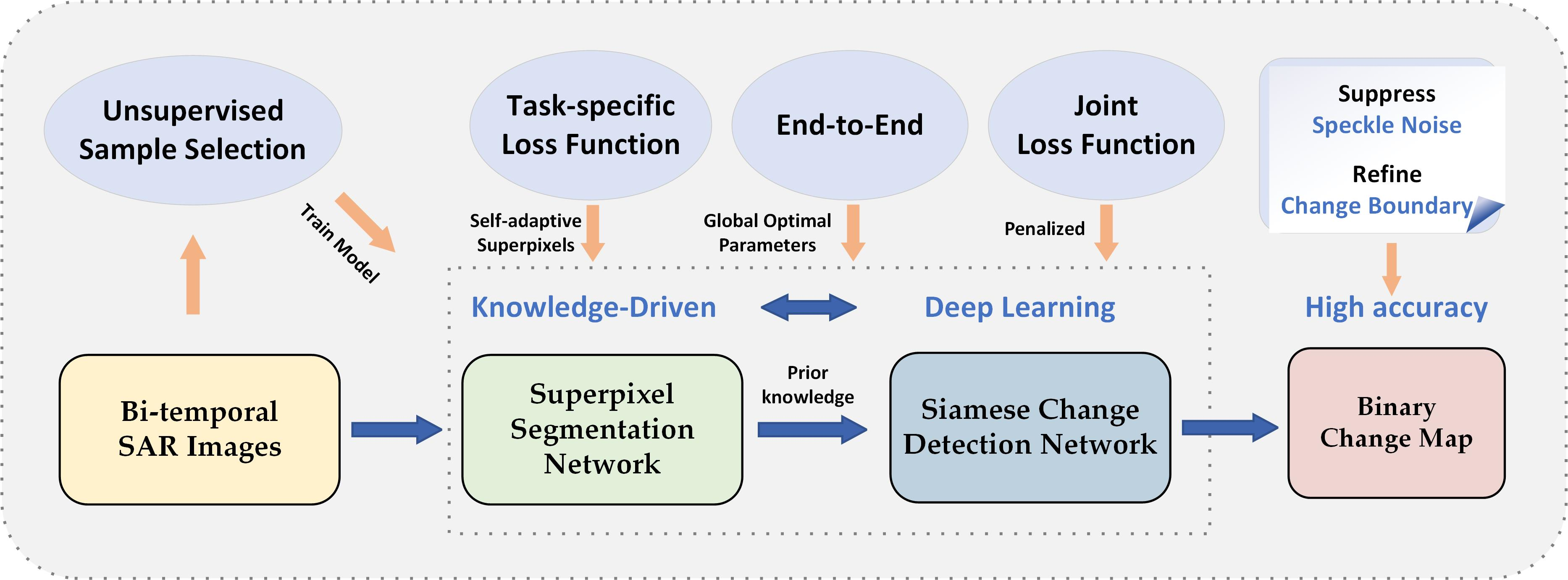
- This study combines knowledge-driven and unsupervised learning to propose an end-to-end CD network. The incorporation of superpixel segmentation information is an interesting practice of integrating prior knowledge into the deep learning technique. The generated superpixels in our proposed method can be adjusted adaptively, which ensures better consistency in the superpixel segmentation of unchanged areas and closer segmentation to change boundaries in changed areas for the bi-temporal data.
- (2)
- This study is the first to explore the ability of the network to detect changes, which is crucial for the generalization performance of CD networks. We designed transfer learning experiments between homogeneous data and even heterogeneous data to explore the ability to detect changes and generalization performance. This information is of great importance for the development of DLCD for SAR images with no or limited samples in the future.
- (3)
- The proposed method is unsupervised and is friendly to SAR data with extremely limited labeled samples. Preprocessed SAR images of different sizes can be input into our network to obtain the change map with high accuracy. Furthermore, this method has the potential to be extended to more complex sequential image processing.
| Algorithms 1: Training steps of the proposed method. |
| Input: Bi-temporal SAR images and Output: The binary change map |
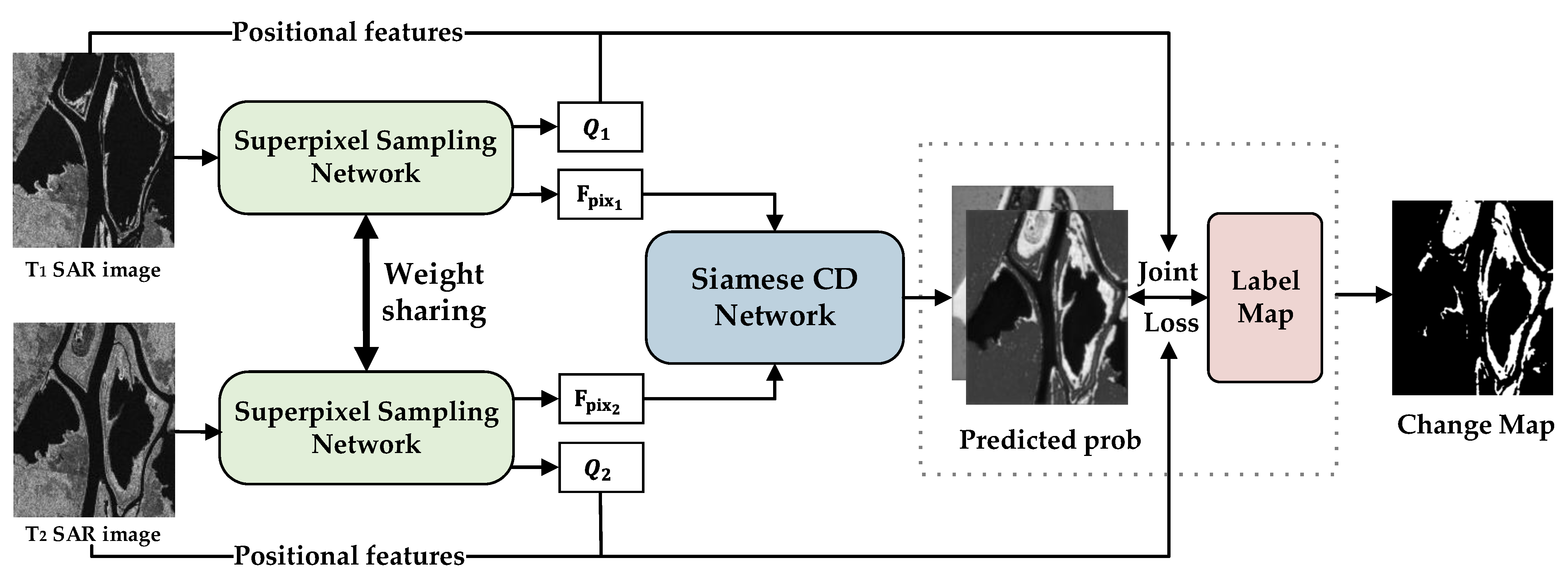
| Normalize the bi-temporal SAR images and for Number of training iterations do 1. Two weight-sharing SSNs take normalized bi-temporal SAR images, respectively, as input. 2. Two SSNs’ output pixel–superpixel associations and and high-level features and for different times. 3. K-dimensional and are fed into the Siamese CD network. 4. The Siamese CD network outputs the predicted probability map . 5. Calculate the weighted cross entropy loss and dice loss as Equations (7) and (9). 6. For both of the different times, calculate task-specific reconstruction loss as Equation (10) and take the positional pixel features of input to calculate compactness loss as Equation (11). 7. Calculate the joint loss as Equation (15). 8. Update the parameters of networks based on the joint loss . End for |
2. Methods
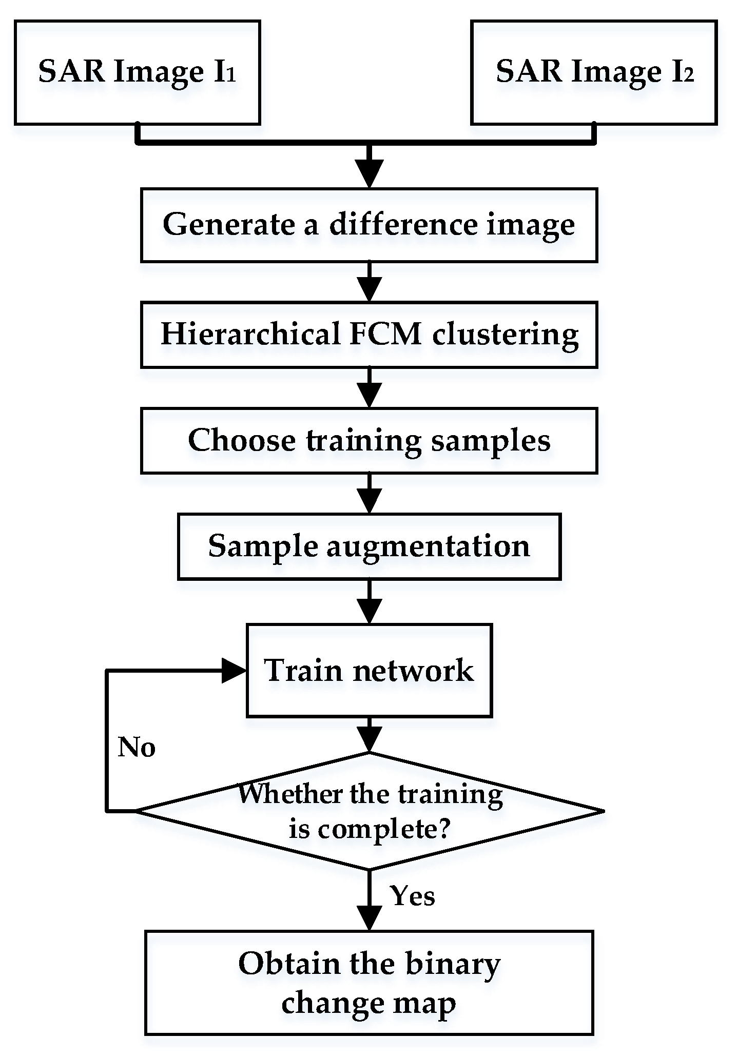
2.1. Unsupervised Change Detection Workflow
2.2. Superpixel Sampling Networks (SSNs)
2.2.1. The Input of the SSN
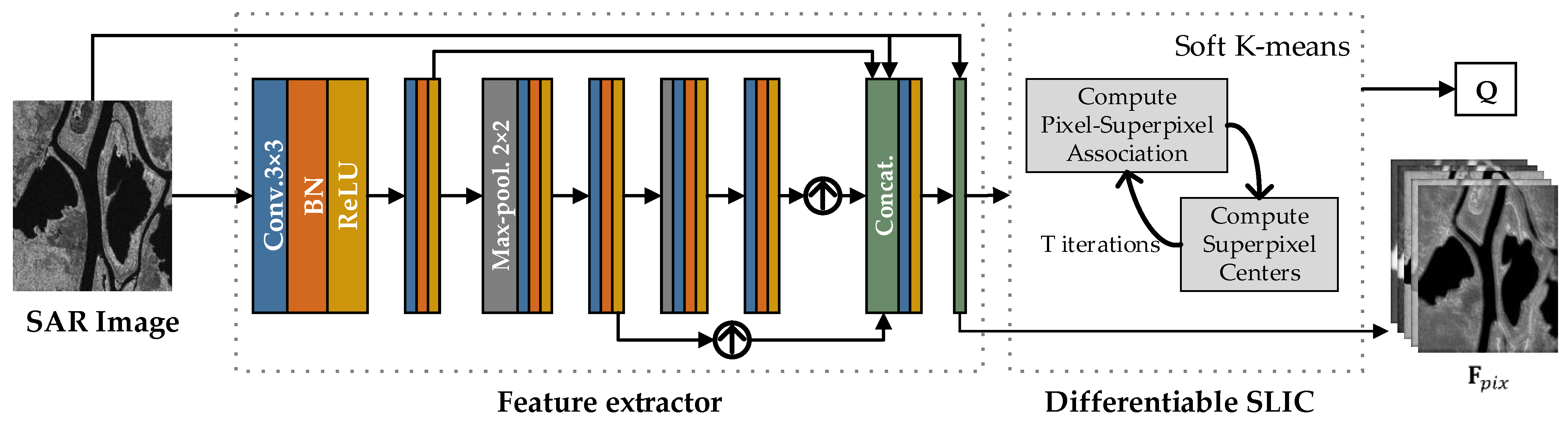
2.2.2. Feature Extractor Based on CNN
2.2.3. Differentiable SLIC
2.3. End-to-End Change Detection Network with SSN
2.3.1. Overall Framework
2.3.2. Siamese CD Network
- FC-Siam-conc
- FC-Siam-diff
2.4. Loss Function
3. Results
3.1. Datasets and Evaluation Criteria
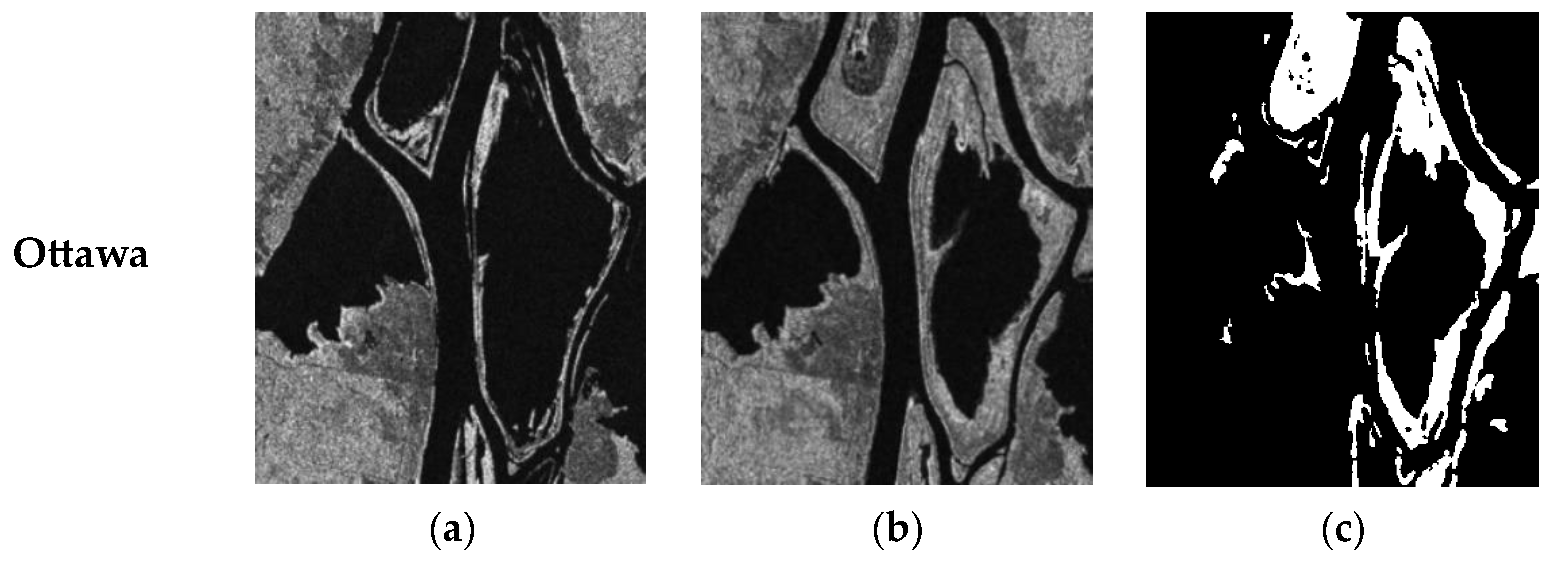
- Ottava dataset: two images were acquired via the Radarsat-1 satellite over Ottawa in May 1997 and August 1997, and the change was caused by the summer flooding (Figure 5).
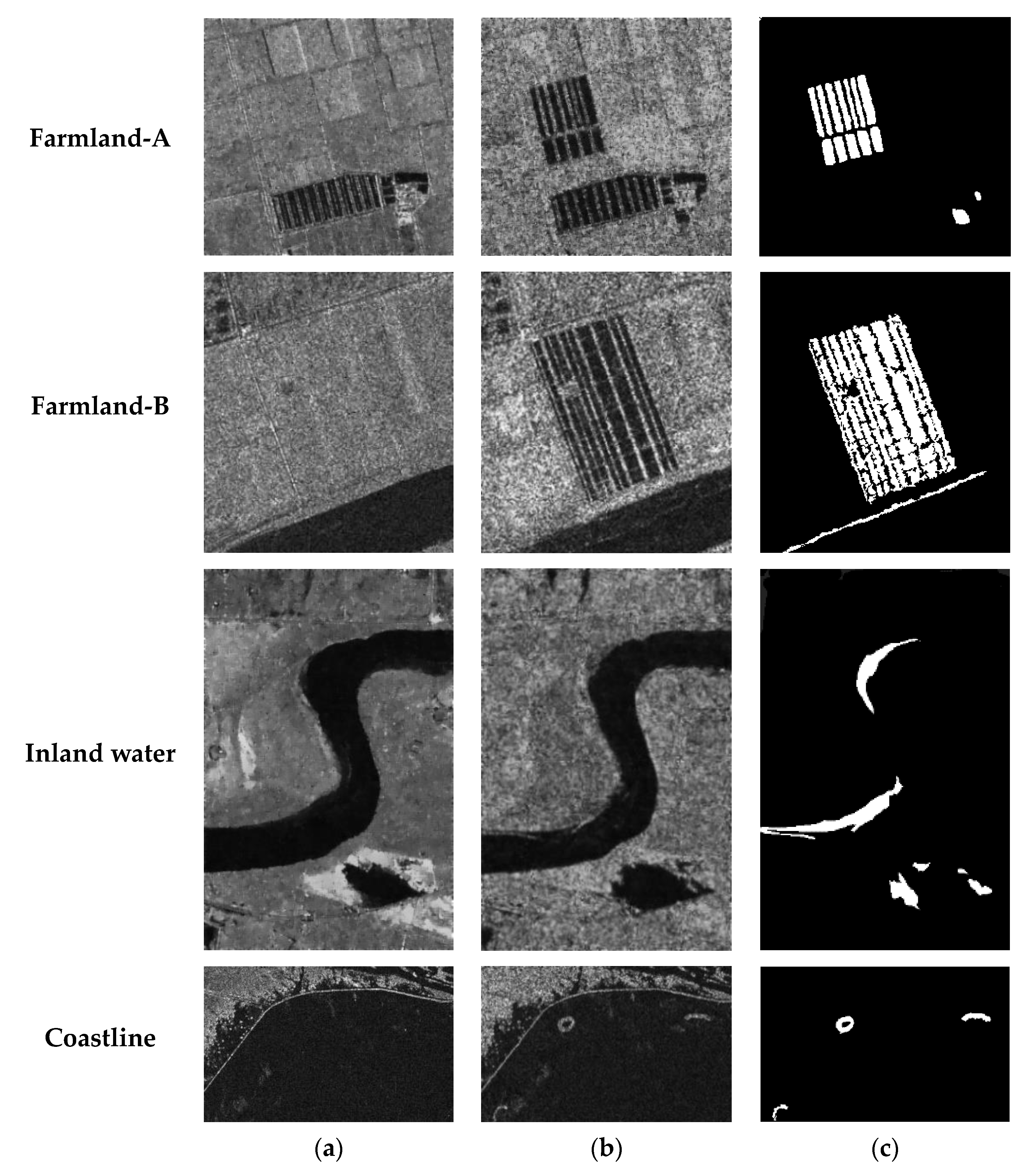
- Yellow River dataset: These two images were acquired via the Radarsat-2 satellite in June 2008 and June 2009 at the estuary of the Yellow River in Dongying, Shandong Province (Figure 7). It is worth noting that the two images are single-look and four-look, respectively. As a result, they are affected by noise to different degrees. Four typical change areas were selected: Farmland-A, Farmland-B, inland water, and coastline dataset.
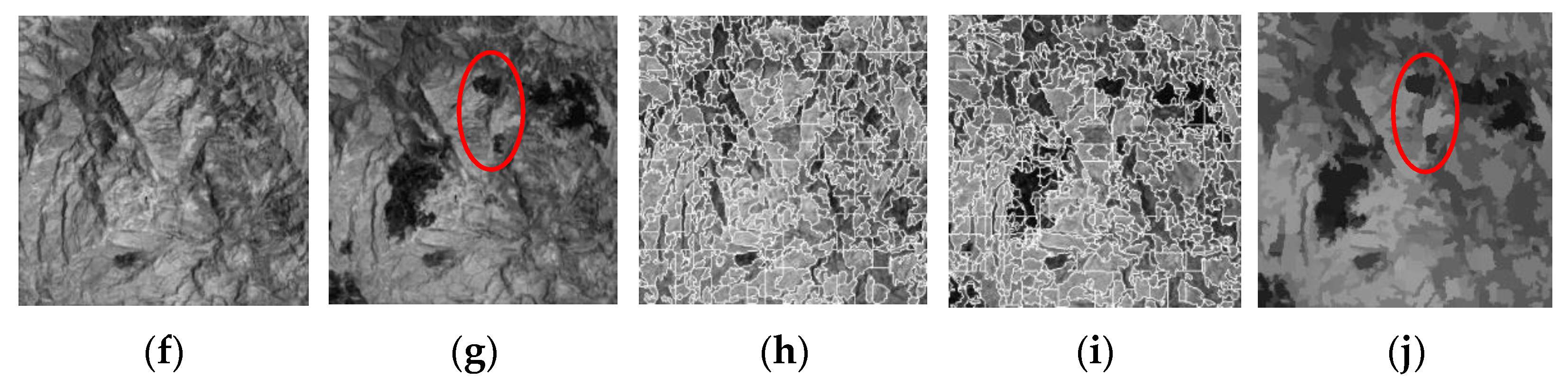
- Mexico dataset: This dataset consists of two optical images captured via Landsat-7 in Mexico City in April 2000 and May 2002, respectively. They were extracted from ETM+ images in band 4, the near infrared (NIR) band. This dataset shows the destruction of vegetation after a forest fire in Mexico city (Figure 9).
3.2. Experimental Setting
3.3. Enhancement Effect in Series with SSN
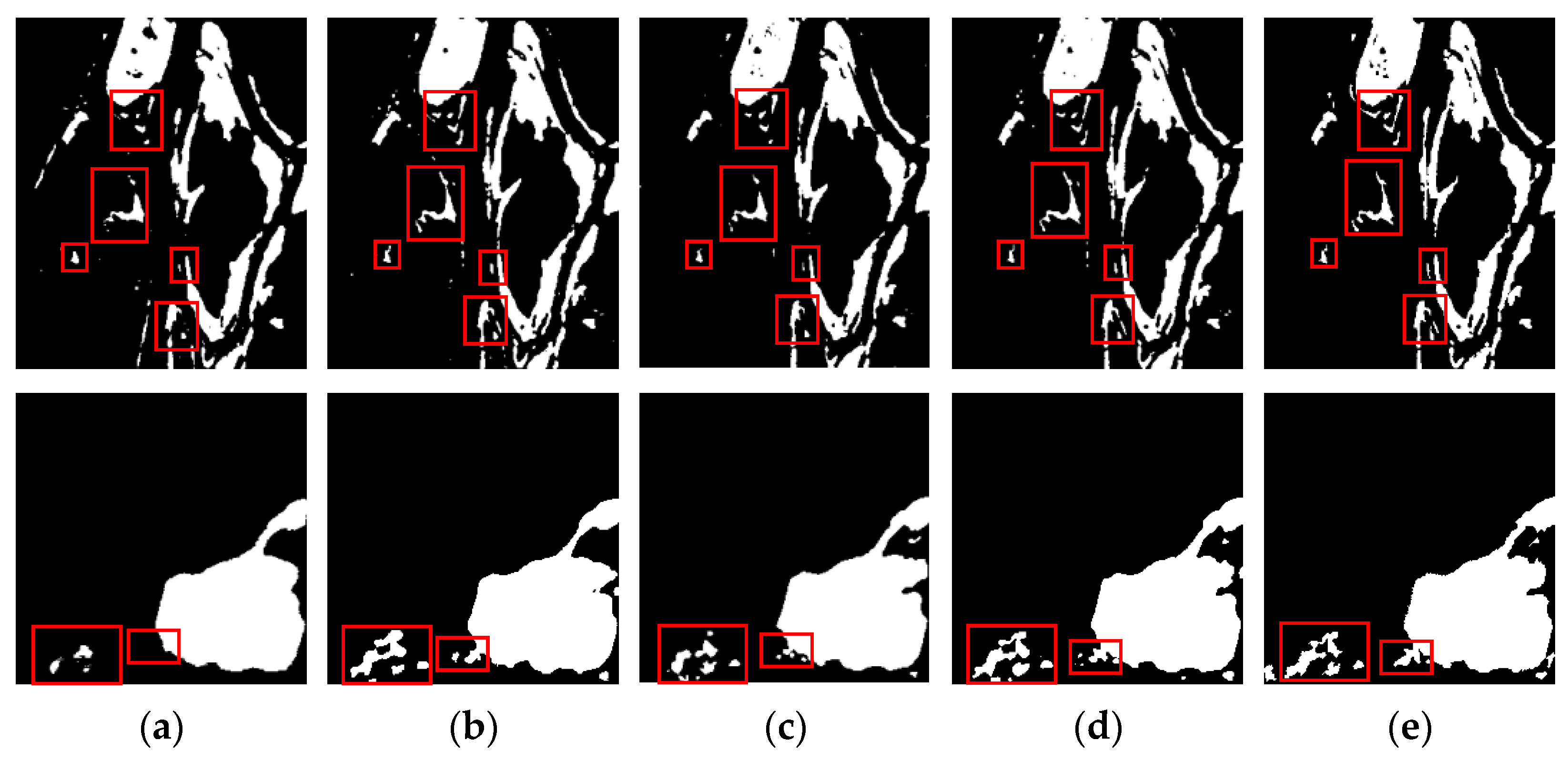
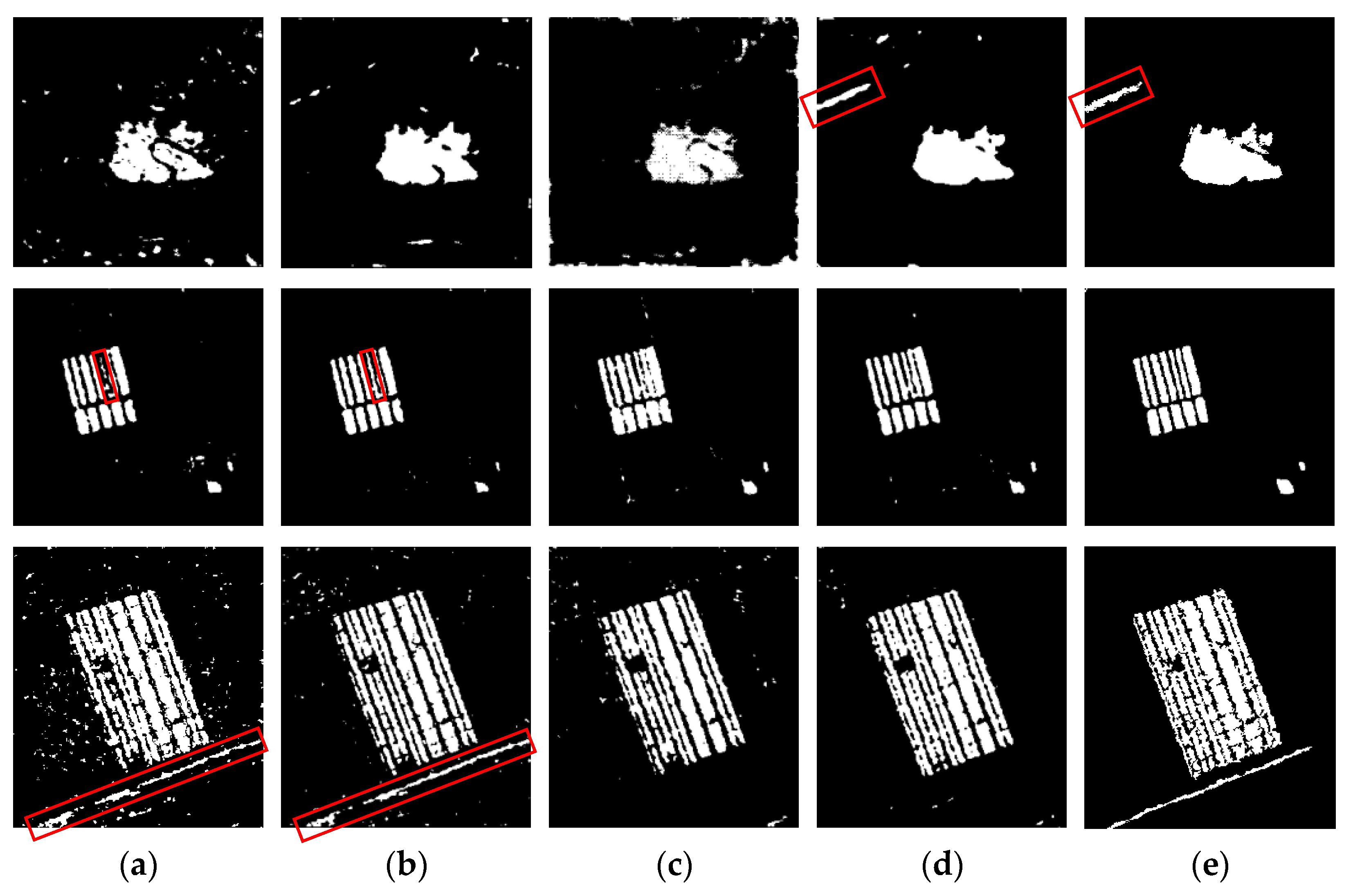
3.3.1. CD Results
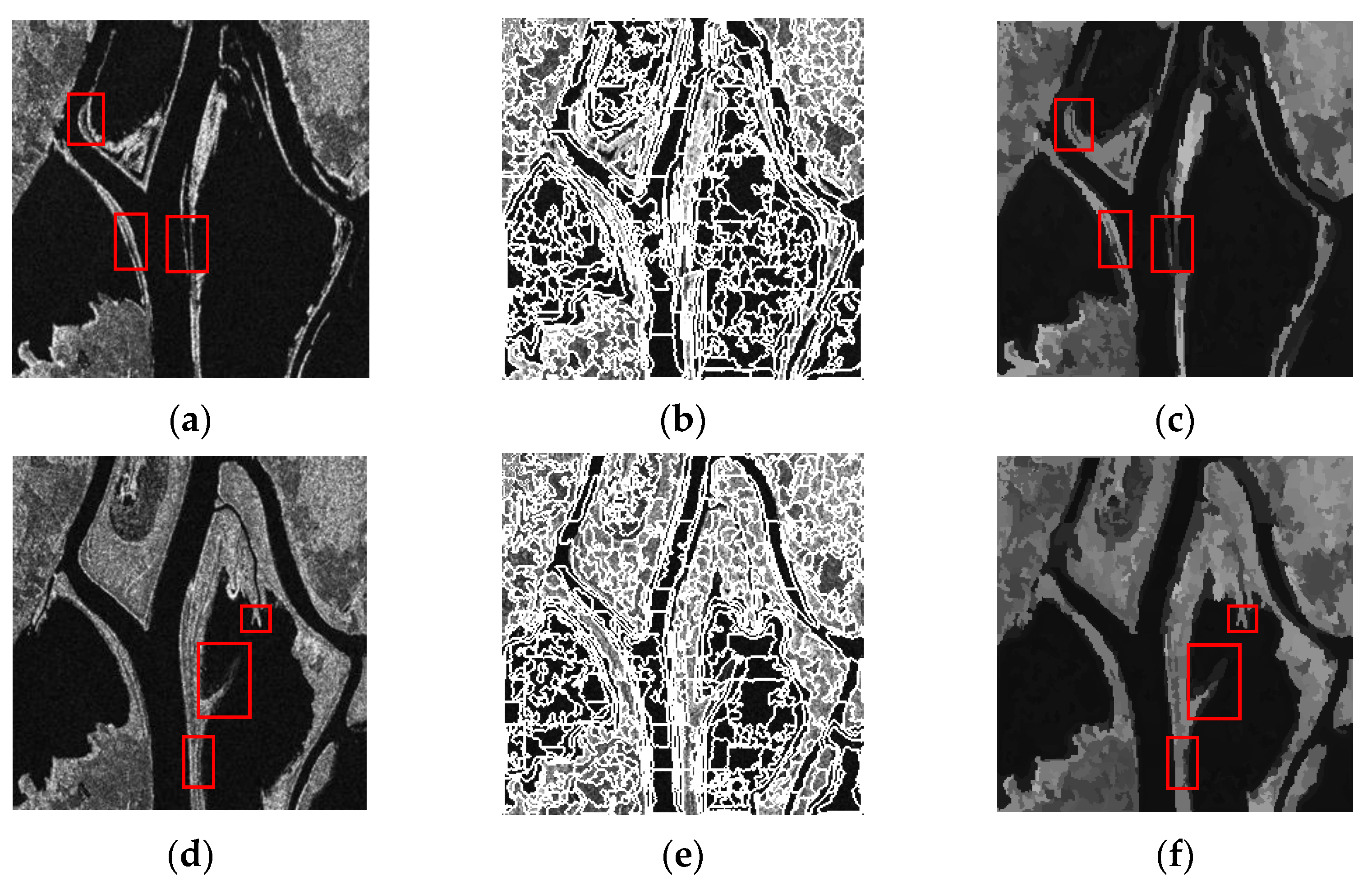
3.3.2. Superpixel Segmentation Results for Bi-Temporal SAR Images
3.4. Transfer Learning Experiments
3.4.1. Transfer Learning for SAR Dataset
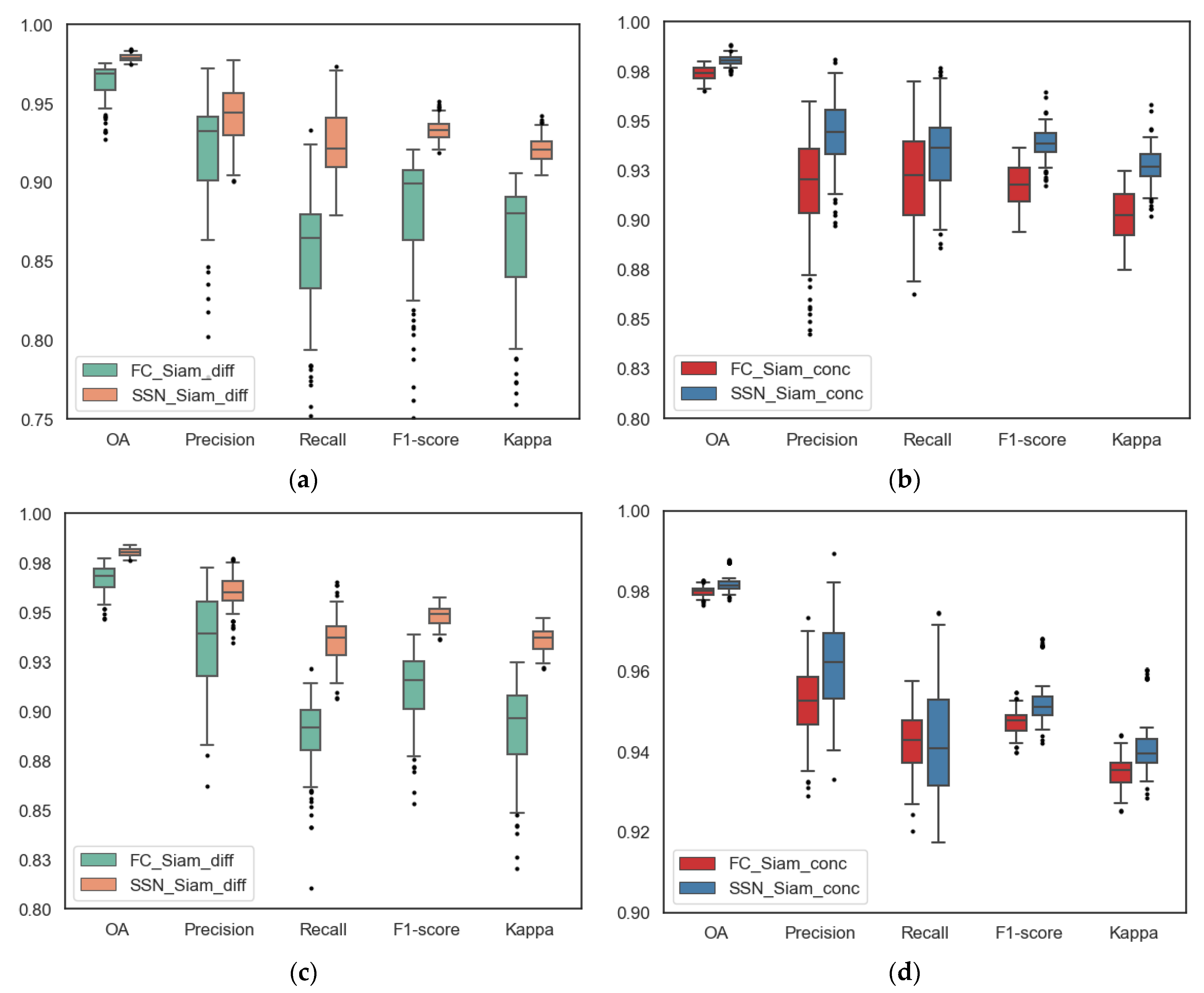
3.4.2. Comparison of Generalization Performance between Conc and Diff Models
3.4.3. Transfer Learning for Optical Dataset
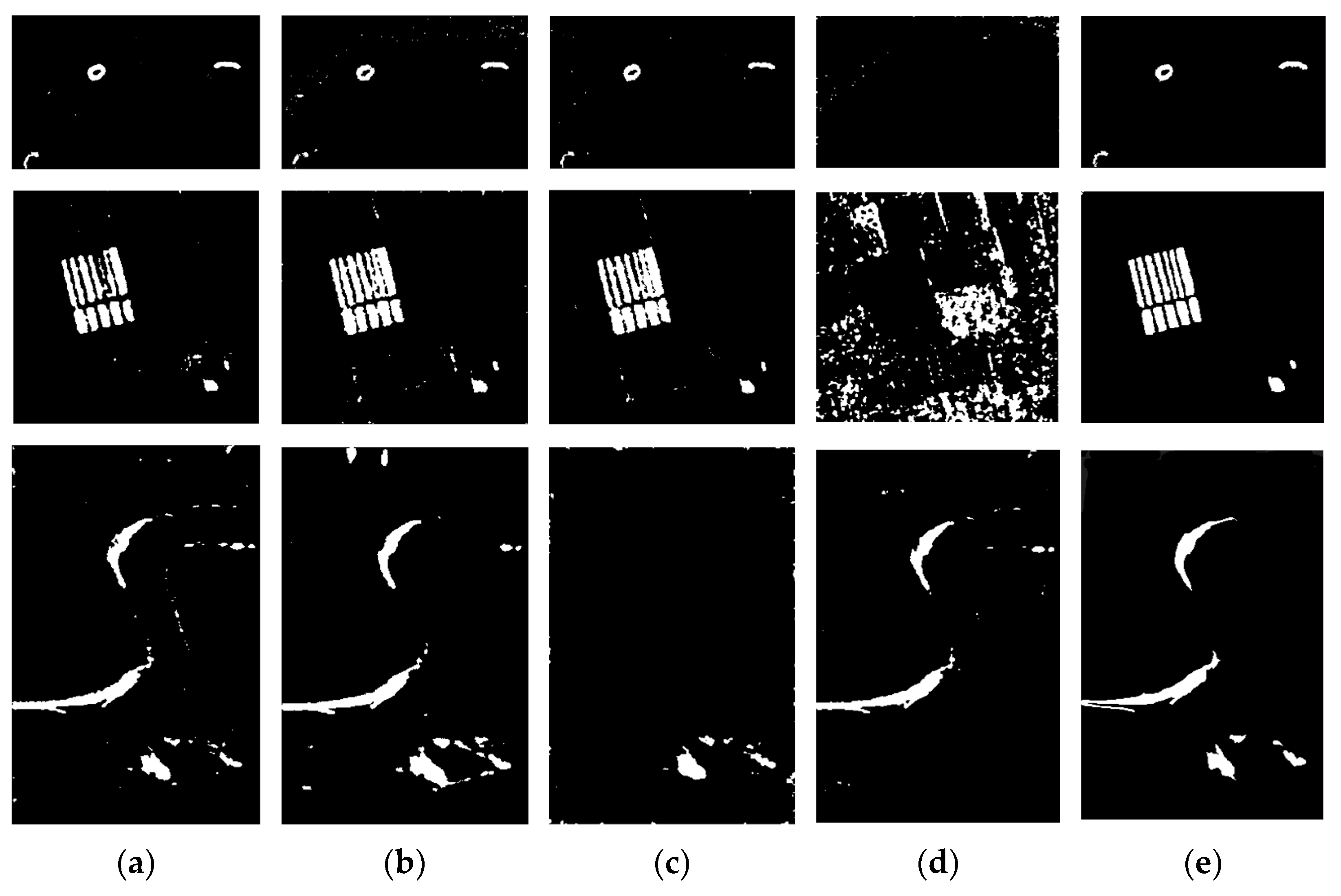
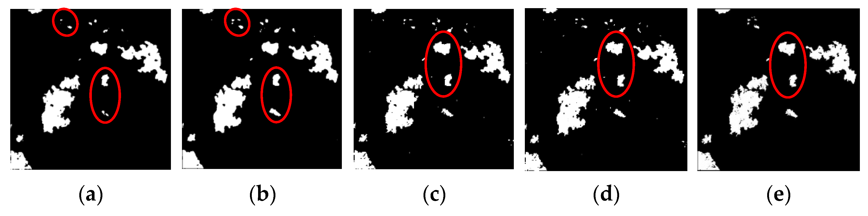
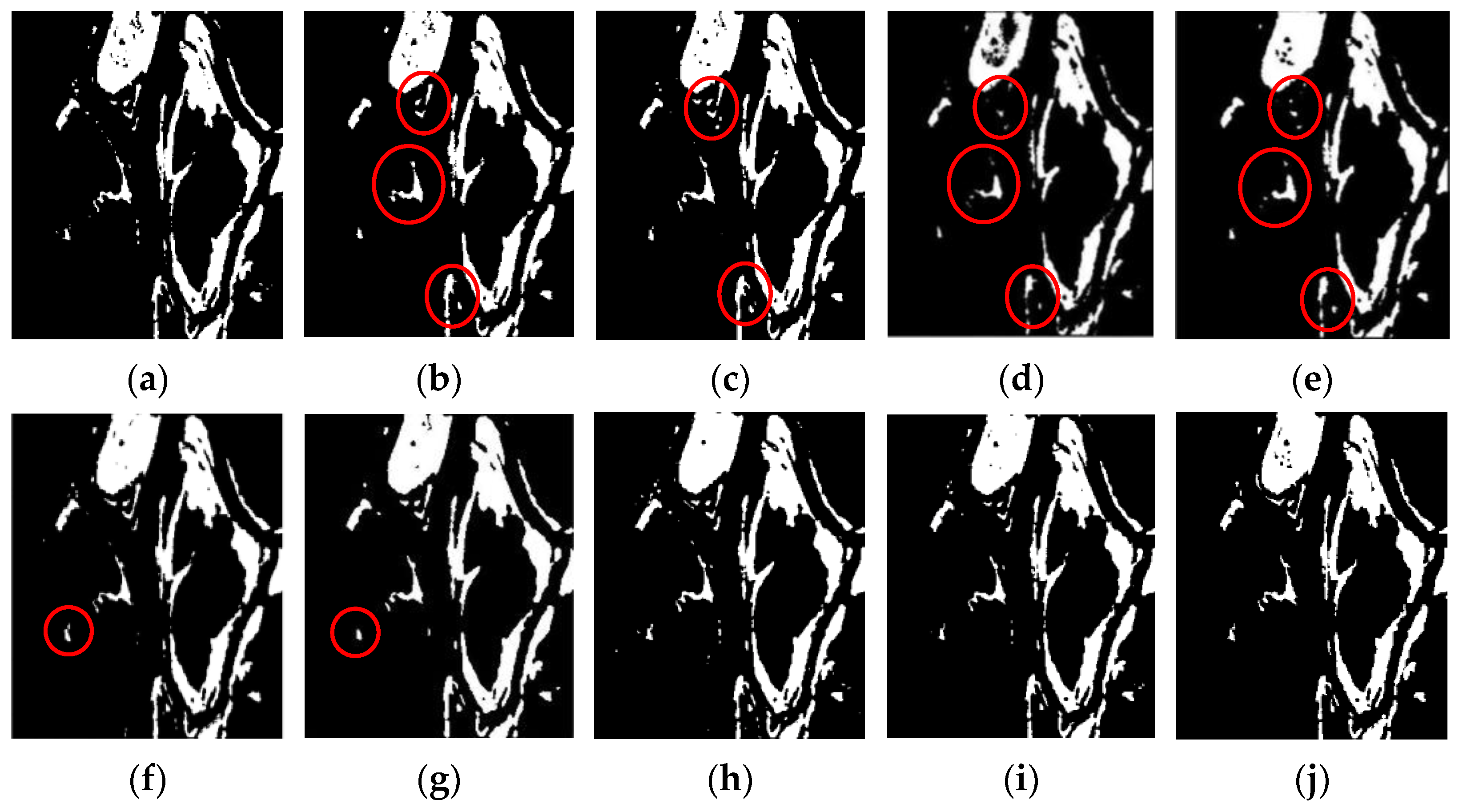
3.5. Comparison with Other Methods
4. Discussion
5. Conclusions
Author Contributions
Funding
Data Availability Statement
Acknowledgments
Conflicts of Interest
References
- Brisco, B.; Schmitt, A.; Murnaghan, K.; Kaya, S.; Roth, A. SAR polarimetric change detection for flooded vegetation. Int. J. Digit. Earth 2013, 6, 103–114. [Google Scholar] [CrossRef]
- Bruzzone, L.; Serpico, S.B. An iterative technique for the detection of land-cover transitions in multitemporal remote-sensing images. IEEE Trans. Geosci. Remote Sens. 1997, 35, 858–867. [Google Scholar] [CrossRef] [Green Version]
- Yousif, O.; Ban, Y. Improving SAR-Based Urban Change Detection by Combining MAP-MRF Classifier and Nonlocal Means Similarity Weights. IEEE J. Sel. Top. Appl. Earth Obs. Remote Sens. 2014, 7, 4288–4300. [Google Scholar] [CrossRef]
- Hu, H.; Ban, Y. Unsupervised Change Detection in Multitemporal SAR Images Over Large Urban Areas. IEEE J. Sel. Top. Appl. Earth Obs. Remote Sens. 2014, 7, 3248–3261. [Google Scholar] [CrossRef]
- Hame, T.; Heiler, I.; San Miguel-Ayanz, J. An unsupervised change detection and recognition system for forestry. Int. J. Remote Sens. 1998, 19, 1079–1099. [Google Scholar] [CrossRef]
- SINGH, A. Review Article Digital change detection techniques using remotely-sensed data. Int. J. Remote Sens. 1989, 10, 989–1003. [Google Scholar] [CrossRef] [Green Version]
- Dekker, R.J. Speckle filtering in satellite SAR change detection imagery. Int. J. Remote Sens. 1998, 19, 1133–1146. [Google Scholar] [CrossRef]
- Yousif, O.; Ban, Y. Improving Urban Change Detection From Multitemporal SAR Images Using PCA-NLM. IEEE Trans. Geosci. Remote Sens. 2013, 51, 2032–2041. [Google Scholar] [CrossRef]
- Hui, Z.; Wang, J.G. A SAR Image Change Detection Algorithm Based on Principal Component Analysis. J. Electron. Inf. Technol. 2008, 30, 1727–1730. [Google Scholar]
- Liu, S.; Du, Q.; Tong, X.; Samat, A.; Bruzzone, L.; Bovolo, F. Multiscale Morphological Compressed Change Vector Analysis for Unsupervised Multiple Change Detection. IEEE J. Sel. Top. Appl. Earth Obs. Remote Sens. 2017, 10, 4124–4137. [Google Scholar] [CrossRef]
- Saha, S.; Bovolo, F.; Bruzzone, L. Building Change Detection in VHR SAR Images via Unsupervised Deep Transcoding. IEEE Trans. Geosci. Remote Sens. 2021, 59, 1917–1929. [Google Scholar] [CrossRef]
- Gong, M.; Li, Y.; Jiao, L.; Jia, M.; Su, L. SAR change detection based on intensity and texture changes. ISPRS J. Photogramm. Remote Sens. 2014, 93, 123–135. [Google Scholar] [CrossRef]
- Rowe, N.C.; Grewe, L.L. Change detection for linear features in aerial photographs using edge-finding. IEEE Trans. Geosci. Remote Sens. 2001, 39, 1608–1612. [Google Scholar] [CrossRef]
- Ma, X.; Liu, S.; Hu, S.; Geng, P.; Liu, M.; Zhao, J. SAR image edge detection via sparse representation. Soft Comput. 2018, 22, 2507–2515. [Google Scholar] [CrossRef]
- Ma, W.; Yang, H.; Wu, Y.; Xiong, Y.; Hu, T.; Jiao, L.; Hou, B. Change Detection Based on Multi-Grained Cascade Forest and Multi-Scale Fusion for SAR Images. Remote Sens. 2019, 11, 142. [Google Scholar] [CrossRef] [Green Version]
- Mastro, P.; Masiello, G.; Serio, C.; Pepe, A. Change Detection Techniques with Synthetic Aperture Radar Images: Experiments with Random Forests and Sentinel-1 Observations. Remote Sens. 2022, 14, 3323. [Google Scholar] [CrossRef]
- Manzoni, M.; Monti-Guarnieri, A.; Molinari, M.E. Joint exploitation of spaceborne SAR images and GIS techniques for urban coherent change detection. Remote Sens. Environ. 2021, 253, 112152. [Google Scholar] [CrossRef]
- Kittler, J.; Illingworth, J. Minimum error thresholding. Pattern Recognit. 1986, 19, 41–47. [Google Scholar] [CrossRef]
- Ghosh, A.; Mishra, N.S.; Ghosh, S. Fuzzy clustering algorithms for unsupervised change detection in remote sensing images. Inf. Sci. 2011, 181, 699–715. [Google Scholar] [CrossRef]
- Krinidis, S.; Chatzis, V. A Robust Fuzzy Local Information C-Means Clustering Algorithm. IEEE Trans. Image Process. 2010, 19, 1328–1337. [Google Scholar] [CrossRef]
- Gou, S.; Yu, T. Graph based SAR images change detection. In Proceedings of the 2012 IEEE International Geoscience and Remote Sensing Symposium, Munich, Germany, 22–27 July 2012; pp. 2152–2155. [Google Scholar]
- Walter, V. Object-based classification of remote sensing data for change detection. ISPRS J. Photogramm. Remote Sens. 2004, 58, 225–238. [Google Scholar] [CrossRef]
- Desclée, B.; Bogaert, P.; Defourny, P. Forest change detection by statistical object-based method. Remote Sens. Environ. 2006, 102, 1–11. [Google Scholar] [CrossRef]
- Bontemps, S.; Bogaert, P.; Titeux, N.; Defourny, P. An object-based change detection method accounting for temporal dependences in time series with medium to coarse spatial resolution. Remote Sens. Environ. 2008, 112, 3181–3191. [Google Scholar] [CrossRef]
- Zhang, H.; Lin, M.; Yang, G.; Zhang, L. ESCNet: An End-to-End Superpixel-Enhanced Change Detection Network for Very-High-Resolution Remote Sensing Images. IEEE Trans. Neural Netw. Learn. Syst. 2021. online ahead of print. [Google Scholar] [CrossRef]
- Sui, H.; Feng, W.; Wenzhuo, L.I.; Sun, K.; Chuan, X.U. Review of Change Detection Methods for Multi-temporal Remote Sensing Imagery. Wuhan Daxue Xuebao Xinxi Kexue BanGeomatics Inf. Sci. Wuhan Univ. 2018, 43, 1885–1898. [Google Scholar]
- Chen, G.; Hay, G.J.; Carvalho, L.M.T.; Wulder, M.A. Object-based change detection. Int. J. Remote Sens. 2012, 33, 4434–4457. [Google Scholar] [CrossRef]
- Ullah, Z.; Usman, M.; Latif, S.; Gwak, J. Densely attention mechanism based network for COVID-19 detection in chest X-rays. Sci. Rep. 2023, 13, 261. [Google Scholar] [CrossRef]
- Ronneberger, O.; Fischer, P.; Brox, T. U-Net: Convolutional Networks for Biomedical Image Segmentation. arXiv 2015, arXiv:1505.04597. [Google Scholar]
- Ullah, Z.; Usman, M.; Jeon, M.; Gwak, J. Cascade multiscale residual attention CNNs with adaptive ROI for automatic brain tumor segmentation. Inf. Sci. 2022, 608, 1541–1556. [Google Scholar] [CrossRef]
- Ullah, Z.; Usman, M.; Gwak, J. MTSS-AAE: Multi-task semi-supervised adversarial autoencoding for COVID-19 detection based on chest X-ray images. Expert Syst. Appl. 2023, 216, 119475. [Google Scholar] [CrossRef]
- Gong, M.; Zhao, J.; Liu, J.; Miao, Q.; Jiao, L. Change Detection in Synthetic Aperture Radar Images Based on Deep Neural Networks. IEEE Trans. Neural Netw. Learn. Syst. 2016, 27, 125–138. [Google Scholar] [CrossRef] [PubMed]
- Daudt, R.C.; Le Saux, B.; Boulch, A.; Gousseau, Y. Urban Change Detection for Multispectral Earth Observation Using Convolutional Neural Networks. In Proceedings of the IGARSS 2018—2018 IEEE International Geoscience and Remote Sensing Symposium, Valencia, Spain, 22–27 July 2018; pp. 2115–2118. [Google Scholar]
- Caye Daudt, R.; Le Saux, B.; Boulch, A. Fully Convolutional Siamese Networks for Change Detection. In Proceedings of the 2018 25th IEEE International Conference on Image Processing (ICIP), Athens, Greece, 7–10 October 2018; pp. 4063–4067. [Google Scholar]
- Chen, J.; Yuan, Z.; Peng, J.; Chen, L.; Huang, H.; Zhu, J.; Liu, Y.; Li, H. DASNet: Dual Attentive Fully Convolutional Siamese Networks for Change Detection in High-Resolution Satellite Images. IEEE J. Sel. Top. Appl. Earth Obs. Remote Sens. 2021, 14, 1194–1206. [Google Scholar] [CrossRef]
- Mou, L.; Bruzzone, L.; Zhu, X.X. Learning Spectral-Spatial-Temporal Features via a Recurrent Convolutional Neural Network for Change Detection in Multispectral Imagery. IEEE Trans. Geosci. Remote Sens. 2019, 57, 924–935. [Google Scholar] [CrossRef] [Green Version]
- Shi, C.; Zhang, Z.; Zhang, W.; Zhang, C.; Xu, Q. Learning Multiscale Temporal—Spatial—Spectral Features via a Multipath Convolutional LSTM Neural Network for Change Detection With Hyperspectral Images. IEEE Trans. Geosci. Remote Sens. 2022, 60, 1–16. [Google Scholar] [CrossRef]
- Ji, L.; Zhao, Z.; Huo, W.; Zhao, J.; Gao, R. Evaluation of Several Fully Convolutional Networks in Sar Image Change Detection. In Proceedings of the ISPRS Annals of the Photogrammetry, Remote Sensing and Spatial Information Sciences; Copernicus GmbH: Hannover, Germany, 2022; Volume X-3-W1-2022, pp. 61–68. [Google Scholar]
- Song, A.; Choi, J.; Han, Y.; Kim, Y. Change Detection in Hyperspectral Images Using Recurrent 3D Fully Convolutional Networks. Remote Sens. 2018, 10, 1827. [Google Scholar] [CrossRef] [Green Version]
- Fang, S.; Li, K.; Shao, J.; Li, Z. SNUNet-CD: A Densely Connected Siamese Network for Change Detection of VHR Images. IEEE Geosci. Remote Sens. Lett. 2022, 19, 1–5. [Google Scholar] [CrossRef]
- Wang, Y.; Gao, L.; Hong, D.; Sha, J.; Liu, L.; Zhang, B.; Rong, X.; Zhang, Y. Mask DeepLab: End-to-end image segmentation for change detection in high-resolution remote sensing images. Int. J. Appl. Earth Obs. Geoinf. 2021, 104, 102582. [Google Scholar] [CrossRef]
- Liu, T.; Yang, L.; Lunga, D. Change detection using deep learning approach with object-based image analysis. Remote Sens. Environ. 2021, 256, 112308. [Google Scholar] [CrossRef]
- Gong, M.; Zhan, T.; Zhang, P.; Miao, Q. Superpixel-Based Difference Representation Learning for Change Detection in Multispectral Remote Sensing Images. IEEE Trans. Geosci. Remote Sens. 2017, 55, 2658–2673. [Google Scholar] [CrossRef]
- Sun, Y.; Lei, L.; Guan, D.; Kuang, G. Iterative Robust Graph for Unsupervised Change Detection of Heterogeneous Remote Sensing Images. IEEE Trans. Image Process. 2021, 30, 6277–6291. [Google Scholar] [CrossRef]
- Achanta, R.; Shaji, A.; Smith, K.; Lucchi, A.; Fua, P.; Süsstrunk, S. SLIC Superpixels Compared to State-of-the-Art Superpixel Methods. IEEE Trans. Pattern Anal. Mach. Intell. 2012, 34, 2274–2282. [Google Scholar] [CrossRef] [Green Version]
- Jampani, V.; Sun, D.; Liu, M.-Y.; Yang, M.-H.; Kautz, J. Superpixel Sampling Networks. arXiv 2018, arXiv:1807.10174. [Google Scholar]
- Rignot, E.J.M.; van Zyl, J.J. Change detection techniques for ERS-1 SAR data. IEEE Trans. Geosci. Remote Sens. 1993, 31, 896–906. [Google Scholar] [CrossRef] [Green Version]
- Gao, F.; Dong, J.; Li, B.; Xu, Q. Automatic Change Detection in Synthetic Aperture Radar Images Based on PCANet. IEEE Geosci. Remote Sens. Lett. 2016, 13, 1792–1796. [Google Scholar] [CrossRef]
- Krizhevsky, A.; Sutskever, I.; Hinton, G.E. ImageNet Classification with Deep Convolutional Neural Networks. In Proceedings of the Advances in Neural Information Processing Systems; Pereira, F., Burges, C.J., Bottou, L., Weinberger, K.Q., Eds.; Curran Associates, Inc.: Red Hook, NY, USA, 2012; Volume 25. [Google Scholar]
- Zhou, Z.; Rahman Siddiquee, M.M.; Tajbakhsh, N.; Liang, J. UNet++: A Nested U-Net Architecture for Medical Image Segmentation. In Proceedings of the Deep Learning in Medical Image Analysis and Multimodal Learning for Clinical Decision Support; Stoyanov, D., Taylor, Z., Carneiro, G., Syeda-Mahmood, T., Martel, A., Maier-Hein, L., Tavares, J.M.R.S., Bradley, A., Papa, J.P., Belagiannis, V., et al., Eds.; Springer International Publishing: Cham, Switzerland, 2018; pp. 3–11. [Google Scholar]
- Gao, F.; Wang, X.; Gao, Y.; Dong, J.; Wang, S. Sea Ice Change Detection in SAR Images Based on Convolutional-Wavelet Neural Networks. IEEE Geosci. Remote Sens. Lett. 2019, 16, 1240–1244. [Google Scholar] [CrossRef]
- Gao, F.; Dong, J.; Li, B.; Xu, Q.; Xie, C. Change detection from synthetic aperture radar images based on neighborhood-based ratio and extreme learning machine. J. Appl. Remote Sens. 2016, 10, 046019. [Google Scholar] [CrossRef]
- Li, Y.; Peng, C.; Chen, Y.; Jiao, L.; Zhou, L.; Shang, R. A Deep Learning Method for Change Detection in Synthetic Aperture Radar Images. IEEE Trans. Geosci. Remote Sens. 2019, 57, 5751–5763. [Google Scholar] [CrossRef]
- Liu, F.; Jiao, L.; Tang, X.; Yang, S.; Ma, W.; Hou, B. Local Restricted Convolutional Neural Network for Change Detection in Polarimetric SAR Images. IEEE Trans. Neural Netw. Learn. Syst. 2019, 30, 818–833. [Google Scholar] [CrossRef]
- Gao, Y.; Gao, F.; Dong, J.; Wang, S. Change Detection from Synthetic Aperture Radar Images Based on Channel Weighting-Based Deep Cascade Network. IEEE J. Sel. Top. Appl. Earth Obs. Remote Sens. 2019, 12, 4517–4529. [Google Scholar] [CrossRef]
- Gao, Y.; Gao, F.; Dong, J.; Du, Q.; Li, H.-C. Synthetic Aperture Radar Image Change Detection via Siamese Adaptive Fusion Network. IEEE J. Sel. Top. Appl. Earth Obs. Remote Sens. 2021, 14, 10748–10760. [Google Scholar] [CrossRef]
- Zhang, X.; Su, H.; Zhang, C.; Gu, X.; Tan, X.; Atkinson, P.M. Robust unsupervised small area change detection from SAR imagery using deep learning. ISPRS J. Photogramm. Remote Sens. 2021, 173, 79–94. [Google Scholar] [CrossRef]


| Items | Ottawa | Sulzberger | Yellow River | San Francisco | Mexico | |
|---|---|---|---|---|---|---|
| Satellite | Radarsat-1 | Envisat | Radarsat-2 | ERS-2 | Landsat-7 | |
| Acquisition time | May 1997– August 1997 | 11 March 2011– 16 March 2011 | June 2008– June 2009 | August 2003– May 2004 | April 2000– May 2002 | |
| Band | Band C | Band C | Band C | Band C | NIR (0.775–0.900) | |
| Size | 290 × 350 | 256 × 256 | Farmland-A: | 306 × 291 | 256 × 256 | 512 × 512 |
| Farmland-B: | 257 × 289 | |||||
| Inland water: | 291 × 444 | |||||
| Coastline: | 450 × 280 | |||||
| Reasons for change | Flood | Sea ice breakup | Environmental change | Unknown | Forest fire | |
| Items | Hyperparameter | Setting | |
|---|---|---|---|
| Ottawa | Sulzberger | ||
| Deep learning universal hyperparameters | Initial learning rate | 0.001 | |
| Optimizer | Adam | ||
| Num epochs | 300 | ||
| Lr_scheduler | StepLR (step_size = 100, gamma = 0.5) | ||
| Regularization | L2 regularization | ||
| Batch size | 1 | ||
| Crop size | 256 | 196 | |
| (SSN) Feature extractor hyperparameters | Base channel | 64 | |
| Output layer channel K | 20 | ||
| (SSN) Differentiable SLIC hyperparameters | Num superpixel | 256 | 196 |
| Num iterations | 10 | ||
| Loss function | , | (0.4, 0.6) | |
| , | (0.0001, 1.0) | ||
| Network | OA (%) | Pre (%) | Recall (%) | F1 (%) | Kappa (%) |
|---|---|---|---|---|---|
| FC-Siam-diff | 97.47 | 91.67 | 92.42 | 92.04 | 90.54 |
| SSN-Siam-diff | 98.42 | 93.00 | 97.35 | 95.13 | 94.19 |
| FC-Siam-conc | 98.01 | 94.83 | 92.47 | 93.64 | 92.46 |
| SSN-Siam-conc | 98.87 | 95.48 | 97.49 | 96.48 | 95.81 |
| Network | OA (%) | Pre (%) | Recall (%) | F1 (%) | Kappa (%) |
|---|---|---|---|---|---|
| FC-Siam-diff | 97.71 | 97.03 | 90.88 | 93.85 | 92.45 |
| SSN-Siam-diff | 98.36 | 95.48 | 96.00 | 95.74 | 94.72 |
| FC-Siam-conc | 98.28 | 96.42 | 94.57 | 95.48 | 94.42 |
| SSN-Siam-conc | 98.77 | 96.20 | 97.45 | 96.82 | 96.05 |
| Network | OA (%) | Pre (%) | Recall (%) | F1 (%) | Kappa (%) |
|---|---|---|---|---|---|
| FC-Siam-diff | 96.62 | 76.83 | 75.43 | 76.12 | 74.30 |
| SSN-Siam-diff | 98.10 | 85.61 | 88.26 | 86.92 | 85.89 |
| FC-Siam-conc | 95.61 | 66.93 | 76.35 | 71.33 | 68.97 |
| SSN-Siam-conc | 98.97 | 91.91 | 93.85 | 92.87 | 92.32 |
| Network | OA (%) | Pre (%) | Recall (%) | F1 (%) | Kappa (%) |
|---|---|---|---|---|---|
| FC-Siam-diff | 98.69 | 93.93 | 83.17 | 88.22 | 87.53 |
| SSN-Siam-diff | 98.88 | 97.43 | 83.30 | 89.81 | 89.22 |
| FC-Siam-conc | 98.80 | 89.30 | 90.63 | 89.96 | 89.32 |
| SSN-Siam-conc | 99.01 | 95.20 | 87.67 | 91.28 | 90.75 |
| Network | OA (%) | Pre (%) | Recall (%) | F1 (%) | Kappa (%) |
|---|---|---|---|---|---|
| FC-Siam-diff | 94.05 | 83.21 | 82.73 | 82.97 | 79.37 |
| SSN-Siam-diff | 95.20 | 89.68 | 82.04 | 85.69 | 82.81 |
| FC-Siam-conc | 94.78 | 90.46 | 78.49 | 84.05 | 80.94 |
| SSN-Siam-conc | 95.01 | 89.09 | 81.50 | 85.12 | 82.13 |
| Network | OA (%) | Pre (%) | Recall (%) | F1 (%) | Kappa (%) |
|---|---|---|---|---|---|
| DBN | 98.83 | 96.45 | 96.14 | 96.29 | 95.59 |
| PCANet | 98.67 | 95.36 | 93.07 | 94.20 | 93.06 |
| CNN | 98.67 | 96.41 | 95.13 | 95.77 | 95.00 |
| LR-CNN | 96.25 | 99.49 | 76.65 | 86.59 | 84.45 |
| DCNet | 98.30 | 95.67 | 93.45 | 94.55 | 93.54 |
| SAFNet | 98.60 | 94.62 | 96.67 | 95.64 | 94.81 |
| RUSACD | 98.13 | 92.06 | 96.51 | 94.24 | 93.12 |
| SSN-Siam-diff (ours) | 98.42 | 93.00 | 97.35 | 95.13 | 94.19 |
| SSN-Siam-conc (ours) | 98.87 | 95.48 | 97.49 | 96.48 | 95.81 |
| Network | OA (%) | Pre (%) | Recall (%) | F1 (%) | Kappa (%) |
|---|---|---|---|---|---|
| DBN | 98.56 | 87.71 | 88.00 | 87.85 | 86.92 |
| PCANet | 96.14 | 61.89 | 90.65 | 73.55 | 71.55 |
| CNN | 98.59 | 92.31 | 83.10 | 87.46 | 87.09 |
| LR-CNN | 98.27 | 81.26 | 91.97 | 86.28 | 85.36 |
| DCN | 98.71 | 90.34 | 87.51 | 88.91 | 88.33 |
| SAFNet | 98.94 | 92.89 | 88.96 | 90.88 | 90.32 |
| RUSACD | 98.67 | 92.49 | 84.12 | 88.10 | 87.65 |
| SSN-Siam-diff (ours) | 98.88 | 97.43 | 83.30 | 89.81 | 89.22 |
| SSN-Siam-conc (ours) | 99.01 | 95.20 | 87.67 | 91.28 | 90.75 |
Disclaimer/Publisher’s Note: The statements, opinions and data contained in all publications are solely those of the individual author(s) and contributor(s) and not of MDPI and/or the editor(s). MDPI and/or the editor(s) disclaim responsibility for any injury to people or property resulting from any ideas, methods, instructions or products referred to in the content. |
© 2023 by the authors. Licensee MDPI, Basel, Switzerland. This article is an open access article distributed under the terms and conditions of the Creative Commons Attribution (CC BY) license (https://creativecommons.org/licenses/by/4.0/).
Share and Cite
Ji, L.; Zhao, J.; Zhao, Z. A Novel End-to-End Unsupervised Change Detection Method with Self-Adaptive Superpixel Segmentation for SAR Images. Remote Sens. 2023, 15, 1724. https://doi.org/10.3390/rs15071724
Ji L, Zhao J, Zhao Z. A Novel End-to-End Unsupervised Change Detection Method with Self-Adaptive Superpixel Segmentation for SAR Images. Remote Sensing. 2023; 15(7):1724. https://doi.org/10.3390/rs15071724
Chicago/Turabian StyleJi, Linxia, Jinqi Zhao, and Zheng Zhao. 2023. "A Novel End-to-End Unsupervised Change Detection Method with Self-Adaptive Superpixel Segmentation for SAR Images" Remote Sensing 15, no. 7: 1724. https://doi.org/10.3390/rs15071724