Remote Sensed and/or Global Datasets for Distributed Hydrological Modelling: A Review

Abstract

This research paper presents a systematic literature review on the use of remotely sensed and/or global datasets in distributed hydrological modelling. The study aims to investigate the most commonly used datasets in hydrological models and their performance across different geographical scales of catchments, including the micro-scale (<10 km²), meso-scale (10 km²–1000 km²), and macro-scale (>1000 km²). The analysis included a search for the relation between the use of these datasets to different regions and the geographical scale at which they are most widely used. Additionally, co-authorship analysis was performed on the articles to identify the collaboration patterns among researchers. The study further categorized the analysis based on the type of datasets, including rainfall, digital elevation model, land use, soil distribution, leaf area index, snow-covered area, evapotranspiration, soil moisture and temperature. The research concluded by identifying knowledge gaps in the use of each data type at different scales and highlighted the varying performance of datasets across different locations. The findings underscore the importance of selecting the right datasets, which has a significant impact on the accuracy of hydrological models. This study provides valuable insights into the use of remote sensed and/or global datasets in hydrological modelling, and the identified knowledge gaps can inform future research directions.

1. Introduction

One of the important issues that the world is facing in the current era is climate change [1], which will have adverse effects on the hydrological cycle of catchments [2]. These effects will not be the same across the world [3], hence their quantification and early prediction effects are important for preparedness. In order to obtain those quantifications, hydrological models are useful tools. The simulations of these models are used by water managers to study the current state of hydrological processes in areas of focus. The development of distributed hydrological models has the potential to provide large-scale predictions [4,5], but these models need to be informed and assessed with distributed observational data for the better representation of spatio-temporal processes [6]. However, one of the main challenges faced by the modellers is the lack of data [7].

Commonly, the in situ data are considered to be the most accurate. However, these ground observations are local and lack the ability to provide proper spatial coverage [8,9,10]. Further, the required huge amount of input data is often not readily and freely available. Luckily, the advancement in remote sensing technologies during the last decade has enabled mankind to gather huge datasets using satellite observations [11,12]. These observations are providing insights about the vast variety of the parameters that are required for building up a hydrological model [13]. The immense diversity of these datasets covers digital elevation maps, land-use maps, soil distribution maps, rainfall, evapotranspiration, soil moisture, leaf area index and others. Moreover, for several of the sources of these datasets, the inventories span back half a century or even more. These freely available datasets are attractive to modellers, as these can fulfill data requirements.

In addition to the model structure, the performance accuracy of a hydrological model is dependent upon the quality of input data. This makes the selection of the right data important. However, the performance of Earth observation (EO) datasets cannot be treated as uniform throughout the globe as it varies across different climatic zones [14]. Moreover, no remote sensed datasets can be regarded as actual observations due to uncertainties being common in them [15]. The quality of such data products needs demonstration [16] and verification with ground observation before use in models [17,18]. With the increasing computing power, adding new data into the inventories of these datasets is happening very rapidly. Because of the abundance in variety and non-uniform performance, the selection of datasets is difficult. Therefore, there is a need to investigate the research that has been conducted in this specific field over the past few years.

Jiang and Wang (2019) [12] performed the overview of the role of satellite-based remote sensing data products in hydrological modelling. However, their study is limited to the exploration of the performance of datasets for flow simulations only. The other model outputs, apart from discharge were not considered. Further, the remotely sensed datasets such as digital elevation models, land-use maps, soil distribution maps and leaf area indices, which are equally important in representing hydrological processes, were not covered by the authors. Likewise, Sheffield et al. (2018) [19] reviewed the current satellite missions and datasets that are being used by national agencies in the regions of Latin American and the Caribbean for water resource management. However, the study is region-specific and the focus is on water resource management instead of distributed hydrological modelling. In both previously mentioned studies, the authors did not mention the years when the publications covered by their review were issued, nor did they describe their methodology for selecting the articles. Additionally, neither study investigated the performance of remote sensed datasets at different geographical scales.

In this paper, we performed a systematic literature review. The aim of study was to investigate the research articles which were published on this topic in six years (2016 to 2021) and which used one or more types of remotely sensed and/or global datasets to establish the distributed hydrological model. More specifically, we aimed to answer the following questions: Which datasets are most widely used by the researchers? At what catchment scale are the remotely sensed datasets mostly used? Have researchers evaluated the performance of these datasets for hydrological simulations? What are the knowledge gaps in this respective field?

To answer the questions, we started the systematic literature review by sourcing 205 articles from Scopus and 208 articles from Web of Science. After that, the final analysis was carried out on 120 articles. Then, we looked into different types of datasets that were used in hydrological models for different catchment sizes. The terms ‘micro-scale’, ‘meso-scale’, and ‘macro-scale’ were used to categorize the sizes of catchments (i.e., less than 10 km² [20]; 10 km² to 1000 km² [21]; and greater than 1000 km² [22], respectively). We performed this to detect the knowledge gaps at each scale concisely. Lastly, we concluded our analysis results and identified the scale-wise knowledge gaps that can act as the way forward for future work in the field.

After this introduction, the paper presents the methodology used for paper selection, which is followed by the results and discussion in Section 3. The paper ends with the Conclusion in Section 4, followed by Appendix A which presents a list of papers categorized.

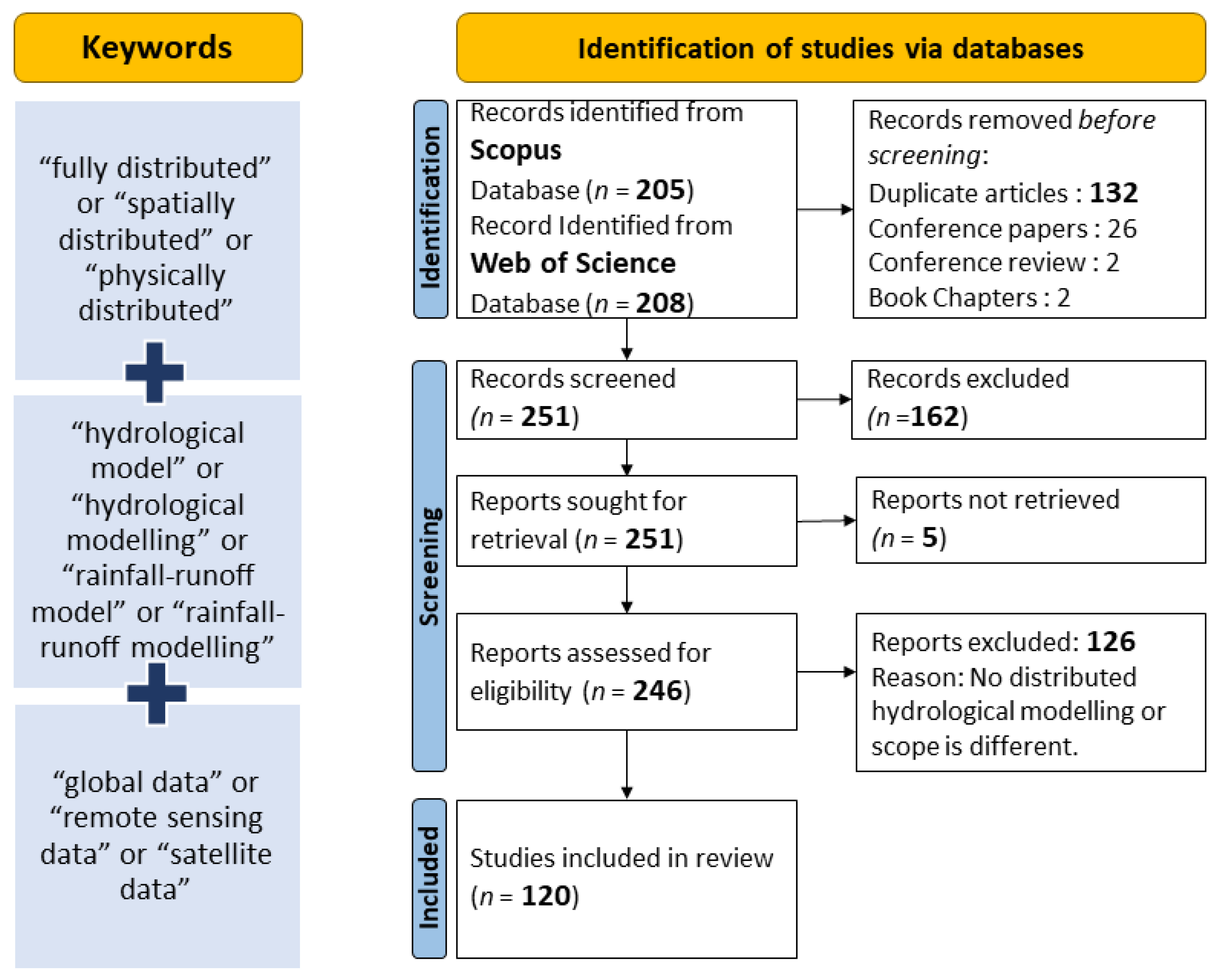
2. Methodology

The review methodology is based on preferred reporting items for systematic reviews and meta-analyses (PRISMA) criteria [23], consisting of three main steps. The first step includes the identification of relevant articles and for that we used the keywords, such as “hydrological modelling”, “remote sensing”, “global data”, etc. All keywords are shown in Figure 1. The process of identification was started by consulting two websites. The first was Scopus and the second was the Web of Science. Studies published between 2016 and 2021 were selected for inclusion in this review to capture the latest advancements and trends in the use of remote sensed and/or global datasets for distributed hydrological modelling and to make the search manageable and feasible. Initially, 413 articles were sourced from the two websites that were mentioned earlier. The second step included the screening of the articles. From the initially sourced 413 articles, some occurred twice because of their presence in both databases, and some were not classified as articles, such as conference papers, conference reviews and book chapters. This reduced the list of articles. Five more articles were excluded as they were not retrievable from the source. After this screening process, we ended up with 246 articles. In the third step, the abstracts of the article were read in order to eliminate the articles with research focuses outside the scope of this review, i.e., detailed distributed hydrological modelling, which included 126 articles. These 126 articles were excluded and the detailed analysis was finally conducted on 120 research articles. The schematic representation of the whole methodological process of selecting the papers for review can be seen in Figure 1.

In the detailed analysis, firstly, the bibliographic analysis was performed to find the link between the regions and/or scale with the use of remote sensed and/or global datasets. Secondly, the shortlisted articles were categorized based on the type of datasets used by the authors for the hydrological modelling. Thirdly, for each dataset type, we further categorized the articles on the basis of catchment scale. Finally, we ascertained the progress of scientific community, both in terms of dataset type and scale.

3. Results and Discussions

In the beginning, we classified the articles country-, region- and scale-wise. The purpose was to analyze the locations around the world where the remote sensed and/or global datasets were being used most. As shown in Figure 2, out of 120 full-text articles reviewed, most studies have been found to be conducted in China, followed by the USA. Conversely, continent-wise, most studies have been conducted in Asia, followed by Europe. If we look at the number of studies conducted at different catchment sizes, then the majority are being performed at the macro-scale.

The main aim of this classification was to find a relationship between the performance of remote sensing datasets and geographic locations, as well as the sizes of catchments. However, after reviewing the literature, we were unable to establish any clear links. For example, we did not find any evidence to suggest that the performance of remote sensing data is consistently better in one region or country over another, such as Asia versus Europe or China versus the rest of the world. However, if we consider the catchment size and number of studies, a direct relationship can then be framed: these studies are more focused on the macro-scale, followed by the meso-scale and micro-scale. Thus, the trend of using remote sensed and/or global datasets in large catchments is more as compared to the use in small ones.

Further, we performed the co-authorship analysis on the articles in order to identify the collaboration patterns among the researchers. For this, VOSviewer software had been used and the method was selected as a full counting method. The threshold of a minimum of two articles by a researcher was chosen as there was no author who had authored three or more articles among the shortlisted articles. Out of 594 authors, only 46 met the threshold. Based on the strength of co-authorship link, 20 clusters were drawn, which are graphically presented in Figure 3.

From Figure 3, it can be seen that there are only three clusters where the number of authors is more than three. The largest clusters are cluster 1 (shown in red) and cluster 2 (shown in green), which have seven authors each. Cluster 3 (shown is blue) is the third largest cluster, with five authors.

The research work of the authors of cluster 1 is focused on assimilation of soil moisture in hydrological models. For cluster 2, the research work is more versatile, covering the subjects of stream flow simulation with limited observed data, the evaluation of satellite-based precipitation products, the merging of satellite-based precipitation products with in situ data, the calibration of hydrological models with limited data and the evaluation of snow melt contribution in catchment hydrological processes. Likewise, the research work of the authors of cluster 3 is focused on flood simulation uncertainty and the uncertainty quantification of satellite-based precipitation for stream flow simulation. However, Figure 3 also represents that there are many authors which have no strong collaborations with others (represented in grey color).

In order to better analyze the contributions of the authors regarding the use of remotely sensed datasets at different scales for the purpose of hydrological modelling, the following discussions have been categorized based on the type of datasets.

3.1. Rainfall Datasets

One of the main components of the water cycle is the rainfall. Given its importance, several efforts have been prompted regarding its estimation and the capture of spatio-temporal variability on earth [24]. For planning and decision making in a variety of disciplines, including hydrology, meteorology, climate, and agriculture, its correct observation is crucial [25]. In hydrological models, precipitation data constitute central input that regulate the spatio-temporal variability of other hydrological fluxes [26].

In recent years, many remote sensed satellite-based rainfall datasets with high spatio-temporal coverage have been produced at a globe scale. These are available in near real time at zero cost [17]. Further, such estimates of precipitation from space are spatially uniform and encompass areas that are difficult to access [27]. However, satellite-based datasets are vulnerable to both systematic and random errors due to various factors. For instance, these datasets are indirectly derived from radiance, which can lead to issues with sampling frequency and the algorithms used for estimation. Additionally, the accuracy of these estimation methods may vary depending on factors such as latitude, altitude, and the type of rainfall being measured [28,29]. Considering these factors, such data products need to be evaluated with observed data.

Among the reviewed articles, there are six studies out of one hundred twenty in which the size of study area is in the range of micro-scale catchment. Only in one study, the authors analyzed the influence of rainfall variability on discharge simulation using physically based distributed hydrological model for small semi urban French catchment. For this study, Paz et al. (2019) [30] used rainfall data from two radars. Unfortunately, at the micro-scale no author used the remote sensed satellite-based rainfall for hydrological modelling. Likewise, there are thirty-two studies in the reviewed articles where the study areas are in the range of meso-scale catchments. Surprisingly, no author used the remote sensed rainfall dataset for setting up a hydrological model even at this scale.

On the macro-scale, the in situ rainfall data have been mostly used, a fact which revealed that the data observed in situ are the first preference of the researchers. Many authors mentioned using remote sensed rainfall data products as well. It is notable that if only different types of remote sensed datasets are compared, then rainfall is among the most used remote sensed dataset. In some of the studies, the authors used both satellite rainfall data products and in situ gauge data in combination. Few authors used the gauge data for the evaluation of satellite-based rainfall products. For instance, for the area of Biliu basin China, Qi et al. (2016) [31] compared six rainfall products statistically with gauge station data and also with respect to hydrological simulation. These products are Tropical Rainfall Measuring Mission (TRMM) versions 3B42 and 3B42RT, Global Land Data Assimilation System (GLDAS), Asian Precipitation-Highly Resolved Observational Data Integration Towards Evaluation of water resources (APHRODITE), Precipitation Estimation from Remotely Sensed Information using Artificial Neural Networks (PERSIANN) and Global Satellite Mapping of Precipitation (GSMaP) products. They developed two hydrological models for the analysis. The first one was fully distributed, while the second one was a semi-distributed hydrological model. The results showed that the APHRODITE rainfall dataset outperformed the five other datasets in statistical comparison with gauge data and also in stream flow simulation by both hydrological models. Likewise, Pakoksung and Takagi (2016) [32] evaluated the performance of five rainfall data products (Global Precipitation Measurement (GPM), GSMaP, TRMM 3B42V7, Climate Prediction Center Morphing technique (CMORPH), and PERSIANN) as an input to rainfall–runoff–inundation (RRI) hydrological model for simulating run-off in the Nan River basin, Thailand. CMORPH and GPM was reported as the best performers based on the statistical comparison with gauge rainfall data while GPM has performed best with respect to stream flow simulation by the model.

As satellite-based rainfall datasets may have some systematic and random errors because of indirect estimation by remote sensing techniques, some researchers tried to correct them based on the use of in situ data. For example, Khairul et al. (2018) [17] evaluated four rainfall products statistically with gauge data. These datasets used were TRMM multi-satellite precipitation analysis (TMPA), Climate Hazards Group InfraRed Precipitation with Station data (CHIRPS), Multi-Source Weighted-Ensemble Precipitation (MSWEP) and GSMaP. They found that all products were weak in apprehending the magnitude and spatial distribution but good in capturing events. They used the merged product of these datasets for hydrological modelling of the Meghna catchment in Bangladesh. However, they did not compare the performance of the merged product with individual datasets in terms of their capability to simulate a hydrological model. Schmied et al. (2021) [33] evaluated the performance of global hydrological model WaterGAP v2.2d based on total water storage anomalies, streamflow and water use using observed data. To simulate the model, they developed the homogenized series of precipitation data using the Water and Global Change (WATCH) forcing data (1901–1978) and WATCH Forcing Data ERA-Interim (WFDEI) (1979–2016). They further adjusted the data to the monthly precipitation sum based on Global Precipitation Climatology Centre (GPCC) data. The authors discussed the effects modifications in the model algorithm and calibration routine had on the results, but did not make any explicit comments on the performance of the model based on the selection of forcing data.

A total of 17 different rainfall products in combination with 6 different temperature datasets are compared by Dembele et al. (2020) [14] as inputs to the meso-scale hydrologic model (mHM) to simulate the hydrological process in the Volta River basin, Africa. The model simulations have been evaluated based on four parameters. These parameters are (1) in situ stream flow data, (2) Global Land Evaporation Amsterdam Model (GLEAM) evaporation data, (3) European Space Agency (ESA) Climate Change Initiative (CCI) soil moisture data and (4) Gravity Recovery and Climate Experiment (GRACE) terrestrial water storage (TWS) data. Among the 17 utilized datasets, no single rainfall dataset ranked first consistently with respect to evaluation parameters. Tropical Applications of Meteorology using SATellite data (TAMSAT), African Rainfall Climatology (ARC), Modern-Era Retrospective analysis for Research and Applications (MERRA-2) and MSWEP are best-performing datasets for streamflow, TWS, soil moisture and actual evaporation simulations, respectively. Lakew et al. (2020) [34] evaluated the performance of five rainfall data products based on their capability to simulate daily flow in three catchments (Gilgel Abbay, Kessie station and Abbay basin) of Ethiopia using the Coupled Routing and Excess STorage (CREST) distributed hydrological model. The used datasets were CMORPH, TRMM TMPA 3B42v7, European Centre for Medium-Range Weather Forecasts (ECMWF) Re-Analysis (ERA) Interim, GPCC and MSWEP. The results indicated that the MSWEP rainfall data product performed better in flow simulation than the rest of them.

Similarly, Singh and Saravanan (2020) [35] evaluated four rainfall products for the Wunna Riveris catchment in India and found that the Global Precipitation Climatology Project (GPCP) rainfall data, TRMM and APHRODITE to be more suitable products for the simulation of hydrological processes in India. Mao et al. (2019) [36] evaluated three rainfall products, namely GLDAS, TRMM, China Meteorological Forcing Dataset (CMFD) and MERRA-2. They assessed that, for runoff simulation, MERRA-2 performed better for the Nujiang River basin, China.

Researchers have used a variety of rainfall datasets in their work. Apart from the examples given above, we listed them in

Table A1. Precipitation datasets used in reviewed articles.

Product	Source	Spatial Extent	Spatial Resolution	Temporal Extent	Temporal Resolution	Articles
Tropical Rainfall Measuring Mission (TRMM) Multi-satellite Precipitation Analysis (TMAP)	S, G	50°N–50°S, 180°W–180°E	0.25°	1998–NP	3-hourly, daily	Macro-scale: Islam et al., (2018) [134]; Khairul et al., (2018) [17]; Singh & Saravanan (2020) [35]; Lakew et al., (2020) [34]; Dembele et al., (2020) [14]; Mao et al., (2019) [36]; Pakoksung & Takagi (2016) [32]; Zhang et al., (2020) [107]; Munzimi et al., (2019) [56]; Luo et al., (2017) [89]; Liu et al., (2017) [135]; Qi et al., (2016) [31]; Ha et al., (2018) [71]; Sun et al., (2018) [136]; Abhishek and Kinouchi (2021) [120]
Multi-Source Weighted-Ensemble Precipitation (MSWEP)	S, G, R	Global	0.1°	1979–NP	3-hourly, daily	Macro-scale: Dembele et al.,, (2020) [14]; Khairul et al., (2018) [17]; Lakew et al., (2020) [34]; Strohmeier et al., (2020) [119]; Beck et al., (2020) [131]; Lakew (2020) [137]; Lazin et al., (2020) [106]; Siqueira et al., (2018) [42]
Tropical Rainfall Measuring Mission (TRMM) Near real time data products (3B42RT or 3B41RT)	S	50°N–50°S, 180°W–180°E	0.25°	1998—NRT	3-hourly, daily	Macro-scale: Dembele et al., (2020) [14]; Leroux et al., (2016) [138]; Shi et al., (2020) [139]; Koppa et al., (2019) [102]; Qi et al., (2016) [31]; Sun et al., (2018) [136]
Climate Prediction Center Morphing technique (CMORPH)	S, G	60°N–60°S, 180°W–180°E	8 km, 0.25°	1998—NRT	3-hourly, daily	Macro-scale: Dembele et al., (2020) [14]; Lakew et al., (2020) [34]; Pakoksung & Takagi (2016) [32]; Leroux et al., (2016) [138]; Shi et al., (2020) [139]; Sun et al., (2018) [136]
Climate Hazards Group InfraRed Precipitation with Station data (CHIRPS)	S, G, R	50°N–50°S, 180°W–180°E	0.05°	1981—NRT	Daily	Macro-scale: Dembele et al., (2020) [14]; Dembele et al., (2020) [68]; Pang et al., (2020) [140]; Khairul et al., (2018) [17]; Ha et al., (2018) [71]
Global Satellite Mapping of Precipitation (GSMaP) Versions 1: Moving Vector with Kalman (MVK) Standard V6 2: Gauge adjusted	R, G	60°N–60°S, 180°W–180°E	0.1°	1: 2001–2013 2: 2000—NRT	Daily	Macro-scale: Dembele et al., (2020) [14]; Khairul et al., (2018) [17]; Pakoksung & Takagi (2016) [32]; Sugiura et al., (2016) [141]; Qi et al., (2016) [31]
Integrated Multi-satellitE Retrievals for Global Precipitation Measurement (GPM) (IMERG)	S, G	60°N–60°S, 180°W–180°E	0.10°	2015—NRT	3-hourly	Macro-scale: Al-Areeq et al., (2021) [69]; Sharif et al., (2017) [57]; Zhang et al., (2020) [107]; Lazin et al., (2020) [106]
Asian Precipitation-Highly Resolved Observational Data Integration Towards Evaluation of water resources (APHRODITE)	S, G, R	55°N–15°S, 60°E–150°E	25 km/0.25°	1951—NRT	Daily	Macro-scale: Islam et al., (2018) [134]; Singh & Saravanan (2020) [35]; Qi et al., (2016) [31]
The National Center for Environmental Prediction (NCEP) Climate Forecast System Reanalysis (CFSR) Soil & Water Assessment Tool (SWAT) Database	R	Global	0.3125°	1979–2014	Daily, monthly	Macro-scale: Alemayehu et al., (2018) [142]; Singh & Saravanan (2020) [35]; Sahoo et al., (2021) [55]
Modern-Era Retrospective analysis for Research and Applications-2 (MERRA-2)	S, G, R	Global	0.625° × 0.5°	1980–NP	Hourly	Macro-scale: Dembele et al., (2020) [14]; Mao et al., (2019) [36]; Gupta and Tarboton et al., (2016) [130]
Precipitation Estimation from Remotely Sensed Information using Artificial Neural Networks (PERSIANN)	S, G	60°N–60°S, 180°W–180°E	0.25°	2000—to NRT	3-hourly	Macro-scale: Pakoksung & Takagi (2016) [32]; Leroux et al., (2016) [138]; Qi et al., (2016) [31]
Global Precipitation Climatology Project (GPCP)	S, G	Global	2.5°, 1.0°	1979—NRT, 1996—2015	Daily, monthly	Macro-scale: Islam et al., (2018) [134]; Singh & Saravanan (2020) [35]
European Centre for Medium-Range Weather Forecasts (ECMWF) Re-Analysis (ERA) Interim	R, G	Global	0.25°	1979–2019	3-hourly, daily	Macro-scale: Lakew et al., (2020) [34]; Hostache et al., (2020) [111]
ERA-5	R	Global	0.25°	1979–NP	Hourly	Macro-scale: Dembele et al., (2020) [14]; Dahri et al., (2021) [70]
Global Land Data Assimilation System (GLDAS)	S, G	90°N–60°S, 180°W–180°E	0.25°	2000–2015	3-hourly	Macro-scale: Mao et al., (2019) [36]; Qi et al., (2016) [31]
African Rainfall Estimation algorithm Version 2 (RFE V2) by National Oceanic and Atmospheric Administration (NOAA)	S, G	Africa 40°N–40°S, 20°W–55°E	0.1°	2001–NP	Daily	Macro-scale: Dembele et al., (2020) [14]; Gupta and Tarboton, (2016) [130]
Global Precipitation Climatology Centre (GPCC)	G	Global	2.5°, 1.0°,0.5° & 0.25°	1891–2016	Daily	Macro-scale: Lakew et al., (2020) [34]; Schmied et al., (2021) [33]
European gridded dataset of daily observations version 20 (E-OBS 20.0)	G	25°N–71.5°N, 25°W–45°E	0.25°	1950–2019	Daily	Macro-scale: Busari et al., (2021) [61]
Global Precipitation Measurement (GPM)	S	Global	0.10°	2014–NRT	Half hourly	Macro-scale: Pakoksung & Takagi (2016) [32]
PERSIANN- Cloud Classification System (CCS)	S	60°N–60°S, 180°W–180°E	0.04°	2003–NP	Hourly	Macro-scale: Li et al., (2019) [84]
PERSIANN- Climate Data Record (CDR)	S, G	60°N–60°S, 180°W–180°E	0.25°	1983–2016	6-hourly	Macro-scale: Dembele et al., (2020) [14]
Tropical Applications of Meteorology using SATellite data (TAMSAT) v3.0	S, G	Africa 38°N–36°S, 19°W–52°E	0.0375°	1983–NP	Daily	Macro-scale: Dembele et al., (2020) [14]
African Rainfall Climatology (ARC) v2	S, G	Africa 40°N–40°S, 20°W–55°E	0.1°	1983–NP	Daily	Macro-scale: Dembele et al., (2020) [14]
The Water and Global Change (WATCH) Forcing Data	R, G	Global	0.5°	1901–2001	Daily	Macro-scale: Schmied et al., (2021)
Watch Forcing Data ERA-Interim (WFDEI) —Corrected using Climatic Research Unit (CRU) data	R, G	Global	0.5°	1979–2018	3-hourly	Macro-scale: Dembele et al., (2020) [14]; Schmied et al., (2021)
WFDEI corrected using GPCC dataset	R, G	Global	0.5°	1979–2016	3-hourly	Macro-scale: Dembele et al., (2020) [14]
Princeton university Global meteorological Forcing (PGF) v3	R, G	Global	0.25°	1948–2012	3-hourly	Macro-scale: Dembele et al., (2020) [14]; Aloysius & Saiers (2017) [143]
Earth20bserve, WFDEI and ERA-Interim merged and bias-corrected (EWEMBI) v1.1	R, G	Global	0.5°	1976–2013	Daily	Macro-scale: Dembele et al., (2020) [14];
Japanese 55-year ReAnalysis (JRA-55)	R	Global	1.25°	1959–NP	3-houly	Macro-scale: Dembele et al., (2020) [14];

G: gauge; S: satellite; R: reanalysis; NP: near present; NRT: near real time.

. Their frequent use advocates their potential worth for hydrological modelling. However, if the aim is to determine one single dataset that is performing well in all catchments, then it is difficult to clearly identify a single product performing better from all perspectives. Datasets vary from catchment on the basis of size and region and depend a lot on evaluation criteria. For instance, either the evaluation criteria are a direct comparison of a dataset with in situ observation, or the criterion is the capacity of a dataset to simulate the hydrological variables. These variables can be runoff, soil moisture, terrestrial water storage, actual evapotranspiration or others. Therefore, it is suggested to test and compare the hydrological simulation capability of different rainfall datasets for the aimed study area rather than relying only on a single dataset.

3.2. Digital Elevations Models

Topography influences the generation of overland flow in the physical hydrological models and is defined by the digital elevation models (DEMs). The river network, slope and drainage area are some of the key characteristics of catchments. These morphological attributes can be estimated by DEMs for representation in distributed hydrological models [37]. Thus, the accuracy of these parameters is directly associated with the precision of DEMs. There are many procedures for the generation of DEMs, including photogrammetry, light detection and ranging systems, satellite optical imagery, SAR interferometry and field surveys. However, remote sensed technologies have the advantage of being relatively less expensive, both in cost and time, at covering larger areas [37,38].

In the reviewed articles, for the micro-scale catchments the authors have only used the national-level datasets for their research. For instance, Ichiba et al. (2018) [39] developed the multi-hydro physically based distributed hydrological model of an urban catchment in France in order to understand the effect of model scale on its hydrological performance. They used the local DEM data from the National Institute of Geographic and Forest Information to carry out the analysis. Likewise, Her and Heatwole (2016) [40] developed the 2D fully distributed hydrological model based on the time–area method to provide an alternative way to simulate hydrological processes. The modelling was performed on the Owl Run catchment using the national elevation data from the United States Geological Survey (USGS).

Similar trends have been observed at the meso-scale, with a greater focus on local or national sources of datasets. Some authors have mentioned using DEM data from the Shuttle Radar Topography Mission (SRTM) and Advanced Spaceborne Thermal Emission and Reflection Radiometer Global Digital Elevation Model (ASTER GDEM) for model development. However, they did not analyze the effect of selecting global DEM datasets on their findings. For macro-scale catchments, the trend of using DEMs is the opposite, with more researchers using global DEMs than local topographic datasets. Out of 79 articles, 52 studies used global DEMs, while only 12 utilized local or national-level topographic datasets. Among the global DEMs, SRTM was the most commonly used product, appearing in 28 articles, followed by the use of ASTER GDEM in 9 articles.

Table A2. Digital Elevation Model datasets used in reviewed articles.

Product	Source	Resolution	Extent	Year of Release	Articles
Spatial Information Shuttle Radar Topographic Mission (SRTM)	S	90 m	60°N–60°S	2003	Micro-scale: None Meso-scale: Macalaldad et al., (2021) [65]; Bugan et al., (2020) [98]; Chen et al., (2016) [67]; Saravanan (2016) [144] Macro-scale: Islam et al., (2018) [134]; Sahoo et al., (2021) [55]; Meng et al., (2018) [145]; Pang et al., (2020) [140]; Busari et al., (2021) [61]; Mao et al., (2019) [36]; Pakoksung & Takagi (2016) [32]; Pakoksung & Takagi (2021) [37]; Soulis et al., (2020) [60]; Watson et al., (2020) [146]; Abdollahi et al., (2017) [147]; Maza el al. (2020) [54]; Yang et al., (2020) [44]; Arthur et al., (2020) [59]; Koo et al., (2020) [148]; Becker et al., (2019) [100]; Pan et al., (2019) [101]; Imhoff et al., (2020) [91]; Siqueira et al., (2018) [42]; Tao & Barros (2019) [149]; Ayala et al., (2020) [41]; Abeysingha et al., (2016) [150]; Hiep et al., (2018) [151]; Li et al., (2019) [152]; Munzimi et al., (2019) [56]; Ha et al., (2018) [71]; Alemayehu et al., (2018) [142]; Zhu et al., (2017) [153]; Schmied et al., (2021)
Advanced Space Borne Thermal Emission and Reflection Radiometer-Global Digital Elevation Model (ASTER GDEM)	S	30 m	83°N–83°S	2009	Micro-scale: None Meso-scale: Mendez-Barroso et al., (2016) [154]; Mimeau et al., (2019) [88]; Gara et al., (2020) [155]; Jaiswal et al., (2020) [156] Macro-scale: Alataway et al., (2019) [58]; Atif et al., (2019) [157]; Cazares-Rodriguez et al., (2017) [158]; Jin & Jin (2020) [103]; Pakoksung & Takagi (2021) [37]; Shi et al., (2020) [139]; Singh & Saravanan (2020) [35]; Zhang et al., (2021) [159]; Zhang et al., (2020) [107].
Global Multi-resolution Terrain Elevation Data 2010 (GMTED 2010)	S, G	225 m	60°N–60°S	2010	Macro-scale: Pakoksung & Takagi (2021) [37]; Dembele et al., (2020) [14]; Dembele et al., (2020) [68].
Hydrological data and maps based on Shuttle Elevation Derivatives at multiple Scales (HydroSHEDS)	S	500 m	60°N–60°S	2009	Macro-scale: Jiang et al., (2020) [81]; Khairul et al., (2018) [17]; Lazin et al., (2020) [106]; Pakoksung & Takagi (2021) [37]; Siqueira et al., (2018) [42]; Schmied et al., (2021)
Global 30 Arc-Second Elevation (GTOPO 30)	S, G	1000 m	90°N–90°S	1993	Macro-scale: Corbari et al., (2019) [133]; Koppa et al., (2019) [102]; Lakew (2020) [137]; Pakoksung & Takagi (2021) [37]
Multi-Error-Removed Improved-Terrain (MERIT) DEM	S	90 m	90°N–60°S	2017	Macro-scale: Pakoksung & Takagi (2021) [37]
TerraSAR-X add-on for Digital Elevation Measurement (TanDEM-X)	S	12 m, 30 m, 90 m	90°N–90°S	2016	Macro-scale: Pakoksung & Takagi (2021) [37]

G: ground based; S: satellite.

lists the different DEMs used by researchers in the reviewed articles.

Out of the reviewed articles, only one study, that of Pakoksung and Takagi (2021) [37], has compared the runoff and inundation area simulation performance of five satellite products for a 2011 flood event in the Nan River basin, Thailand, through distributed hydrological modelling. The datasets used were SRTM, ASTER GDEM, Global Multi-resolution Terrain Elevation Data 2010 (GMTED 2010), Global 30 Arc-Second Elevation (GTOPO-30) and Hydrological data and maps based on Shuttle Elevation Derivatives at multiple Scales (HydroSHEDS). For the simulation of run-off, GMTED 2010 performed comparatively better, while SRTM gave the highest accuracy for inundation area simulation. Although GMTED 2010 has a coarser resolution (1000 m by 1000 m), it performed better in run-off simulation as compared to other finer-resolution data products, whereas SRTM performed better for inundation area imitation. Some researchers have utilized multiple data products to cater to their utility needs. For instance, Ayala et al. (2020) [41] used local 55 m contour lines, SRTM, and TanDEM-X datasets to extract DEMs for the years 1955, 2000, and 2013, respectively. They used the derived DEM for glacier change and runoff studies in the Maipo River basin, Chile. Similarly, Siqueira et al. (2018) [42] used SRTM DEMs and HydroSHEDS data for flow accumulation. However, in these studies, the authors did not perform any performance evaluation.

The analysis showed that the use of global DEM datasets in the hydrological models is a common practice among the researchers. It is the only dataset where the use of remote sensed-derived global products has exceeded the use of local or national datasets. DEM is one of the essential inputs to the models and the accuracy of many terrain features, such as extents, slopes, elevations, is dependent on the accuracy of DEM. Despite its importance, only one study among the reviewed article is focused on the hydrological evaluation of different global DEMs [37]. However, this study was limited to a macro-scale catchment and there is a lack of such evaluations for micro- and meso-scale catchments. The selection of a suitable source of DEM is an important step in the hydrological modelling procedure and the dearth of literature in this respect is concerning.

3.3. Land-Use Land-Change Datasets

Land cover plays a vital role in hydrology as it defines the properties of land surface in the models. In the physically based models, land cover represents the distribution of vegetation over the area which is used to calculate the spatial and temporal distribution of actual evapotranspiration (AET). In the overland component of models, the resistance to flow is represented by Manning values, which are often linked with the land-use type. Studies showed that the major portion of earth’s surface is altered due to human’s activities [43] and these changes are also represented in models through land-use land-change (LULC) maps. In recent years, there has been a proliferation of global-scale LULC datasets produced using remote sensing techniques. Despite the fact that these LULC datasets give a typical reflection of the Earth’s surface, they still differ in certain ways, such as in the methodology used to collect data and to construct land-use maps, the number and type of sensors used for detections, their spatial resolution, and their classification definition [44]. Nevertheless, many countries have developed their local- or national-level LULC datasets using classification techniques based on fine-resolution aerial or satellite images. Even though these products may be regarded as the best datasets to be input into hydrological models, their availability and quality cannot always be guaranteed [45].

Among the reviewed articles, researchers have primarily used local- or national-level data products for all three catchment scales. At the meso-scale, the most frequent used regional or global data product is the Coordination of Information on the Environment (CORINE) land-cover map which has a spatial resolution of 100 m [46,47,48]. For studies conducted in the USA, the National Land Cover Database (NLCD), produced by USGS and with a spatial resolution of 30m, is the most commonly used dataset [49,50,51].

At the macro-scale, the most commonly used LULC dataset among the reviewed articles is the Global Land-Cover Characteristics (GLCC) by USGS (in 8 articles), followed by Globcover by ESA (in 7 articles), CORINE land-cover by Copernicus (in 5 articles) and moderate-resolution imaging spectroradiometer (MODIS) Terra+Aqua land-cover products (in 5 articles). The different LULC datasets used by researchers in the reviewed articles are tabulated in

Table A3. Land-Use/Land-Change (LULC) datasets used in reviewed articles.

Product	Source	Spatial Resolution	Extent	Temporal Extent & Resolution	Articles
Globcover by European Space Agency (ESA)	S	300 m	Global	N/A	Meso-scale: Appel et al., (2019) [66] Macro-scale: Dembele et al., (2020) [14]; Dembele et al., (2020) [68]; Islam et al., (2018) [134]; Busari et al., (2021) [61]; Siqueria et al., (2018) [42]; Cobari et al., (2019) [133]; Ha et al., (2018) [71]
Global Land-Cover Characteristics (GLCC) by United States Geological Survey (USGS)	S	1000 m	Global	N/A	Meso-scale: Macalalad et al., (2021) [65]; Chen et al., (2016) [67] Macro-scale: Mao et al., (2019) [36]; Pakoksung & Takagi (2016) [32]; Pakoksung & Takagi (2021) [37]; Koo et al., (2020) [148]; Hiep et al., (2018) [151]; Li et al., (2019) [84]; Koppa et al., (2019) [102]; Qi et al., (2016) [31].
MODIS (Moderate Resolution Imaging Spectroradiometer) / Terra + Aqua Land Cover Type	S	500 m	Global	Yearly, 2001–2019	Meso-scale: Abiodun et al., (2018) [80] Macro-scale: Busari et al., (2021) [61]; Dahri et al., (2021) [70]; Lazin et al., (2020) [106]; Tao & Barros (2019) [149]; Cazeres-Rodriguez et al., (2017) [158]
Coordination of Information on the Environment (CORINE) land cover	S	100 m	Europe	1990, 2000, 2012, 2018	Meso-scale: Hebe et al., (2017) [47], Hollering et al., (2017) [48], Cenci et al., (2016) [46] Macro-scale: Busari et al., (2021) [61]; Chalkidis et al., (2016) [160]; Soulis et al., (2020) [60]; Huang et al., (2019) [18]; Imhoff et al., (2020) [91]
Land-cover classification gridded maps by Climate Data Store (CDS) Copernicus	S	300 m	Global	Yearly, 1992–NP	Meso-scale: Teweldebrhan et al., (2018) [87] Macro-scale: None
Global Land Cover 2000 by Joint Research Centre (JRC)	S	1000 m	Global	2000	Macro-scale: Aloysius & Saiers (2017) [143]

G: gauge; S: satellite; R: reanalysis; NP: near present.

.

The literature shows that new LULC datasets can be prepared for specific areas by using techniques such as supervised, unsupervised and semi-supervised classification algorithms. For instance, Wang and Chen (2019) [52] used the Landsat-8 satellite imagery to develop the land-cover maps for the Shahe Creek in Guangzhou, China, using support vector machine (SVM) algorithms, which are a type of supervised classification technique. They identified the key hydrological processes for flood forecasting by setting up the distributed hydrological model using the land-use map developed. Similarly, Gampe et al. (2016) [53] derived the LULC map for the Gaza Strip from SPOT-5 satellite images, which are made to be used in a water balance simulation model (WaSiM) to assess future drought risk. However, they did not mention the technique used for the development of land-use maps.

Similarly, at the macro-scale, Maza et al. (2020) [54] used (Linear Imaging Self-Scanning-IV) LISS-IV satellite images for the development of two LULC maps for the Kangsabati reservoir catchment India. The first had 8 vegetation classes, while the second had 16 vegetation classes. The study showed that the variable infiltration capacity (VIC) hydrological model, having a fine land-use dataset with 16 vegetation classes, had performed better in low as well as in high flows. Sahoo et al. (2021) [55], Singh and Saravanan (2020) [35] and Munzimi et al. (2019) [56] used Landsat satellite images data to derive the LULC maps. Sharif et al. (2017) [57] and Alataway and El Alfy (2019) [58] used the satellite imagery data from the Landsat satellite as well as from the SPOT-5 satellite images for the development of the LULC map. Likewise, Arthur et al. (2020) [59] used images data from Landsat satellite and MODIS satellite to derive the LULC map. These authors mentioned the development of land-cover maps using the satellite images, but they did not analyze the accuracy of using the specific algorithm to compile them or how this affects hydrological simulations.

Although global land-cover datasets are widely used, they may lack specific land-cover classifications that are required for certain studies, such as glacier coverage, crop type, etc. In light of this, some researchers have modified global land-cover maps by incorporating additional data sources to achieve the necessary specificity for their particular study. For instance, Mao et al. (2019) [36] modified the GLCC data with glacier coverage data from the International Center for Integrated Mountain Development (ICIMOD) for Nujiang River basin, China. Similarly, Soulis et al. (2020) [60] updated the CORINE land cover with data from the Integrated Administration and Control System, Greece, (IACS) for the agricultural part to be used in the distributed hydrological modelling of Greece. However, no author evaluated the effect of LULC data source on the hydrological simulations. Only Busari et al. (2021) [61] studied the effect of incorporating the multiple LULC maps into hydrological modelling. They developed two physically based distributed hydrological models using mHM modelling software for the Karasu Basin in Turkey. The first model was based on a single dataset of LULC from Globcover, while the second model was based on multiple LULC datasets sourced from CORINE for years 1990 and2000 and from the MODIS land-cover product for years from 2001 to 2008. The research concluded that the model with multiple LULC datasets (dynamic) had better performance in flow prediction at outlet than the model having static information of the land use.

One of the crucial inputs in hydrological modelling is LULC data, and their usefulness needs to be carefully assessed. The common goal of the development of global LULC datasets is to develop a harmonized coverage for the whole globe that can be used for studies related to environmental assessment and climate change. The key characteristic of each initiative is that it is ensured that the same technique and classification rule is applied for the whole area. These exclusive properties make these products perfect inputs for hydrological modelling across different areas of the world. However, their taxonomy and class definition differ, resulting in a different legend [45]. The typical way of mapping LULC is through the use of field surveys. However, mapping at the catchment scale is time consuming and expensive, and in many cases is not practical [52]. The applicability of global datasets to simulate hydrological models must be analyzed in order to understand their performance in comparison to that of fine-resolution LULC datasets. Further, it is required to determine up to what standard these global datasets may be utilized as an alternative or as the only source in the data-scarce regions. Moreover, the literature review also depicts that there is a lack of such investigations.

3.4. Soil Distribution and Properties Datasets

Soil is one the dominant factors in regulating the hydrology of the catchment as it controls the streamflow generation, defines the flow path and influences the water balance. This makes the soil information an important input for physically based hydrological models [62]. The limited availability of distributed soil information is common around the globe. This may be because the traditional soil survey methods are time consuming and expensive [63]. Moreover, the soil information is not often readily available in formats suitable for inclusion in models [64]. During recent years, many global-scale soil distribution and properties datasets have been produced by many agencies with the aim to provide harmonized soil information coverage throughout the earth’s surface. At the same time, many countries have their own soil information and properties databases.

Among the reviewed articles, researchers have primarily used soil information data from local or national databases for all three catchment scales. For instance, Ichiba et al. (2018) [39] used the local soil data from the Bureau de Recherches Géologiques et Minières database for setting up the multi-hydro physically based distributed hydrological model of an urban micro-scale catchment in France. Similarly, Her and Heatwole (2016) [40] used the national soil data from soil survey geographic database (SSURGO) for the hydrological modelling on Owl Run catchment, USA. It is important to mention that none of the reviewed articles used any global soil information dataset for micro-scale catchments.

At the meso-scale, few researchers mentioned using the global soil information datasets such as Digital Soil Map of the World (DSMW) by Food and Agriculture Organization (FAO) [65], Harmonized World Soil Database (HWSD) [66] and SoilGrids—global gridded soil information—by ISRIC (International Soil Reference and Information Centre) with a 1000m resolution [67]. In one study, Wang and Chen (2019) [52] noted that DSMW by FAO is not a recent dataset. Thus, the authors updated it based on the land-cover data and used it for hydrological model setup to identify the key hydrological process in the highly developed Shahe Creek catchment, China. However, in these studies, none of the authors evaluated the effect of soil-related datasets used at the meso-scale on hydrology.

At the macro-scale, the number of studies that have used the global soil datasets as compared to one using local soil inventories for distributed hydrological modelling are more. The most frequently used global products for soil distribution information are DSMW by FAO (13 articles), followed by its updated version HWSD (11 articles), SoilGrids by ISRIC (9 articles) and European Soil Database (ESDB) by European Soil Data Centre (ESDAC) (3 articles). The different datasets used by authors in the reviewed articles are tabulated in

Table A4. Soil distribution and properties datasets used in reviewed articles.

Product	Source	Spatial Resolution	Extent	Articles
FAO Digital Soil Map of the World (DSMW)	G	1000 m	Global	Meso-scale: Macalalad et al., (2021) [65]; Wang and Chen (2019) [52] Macro-scale: Ha et la. (2018) [71]; Islam et al., (2018) [134]; Arthur et al., (2020) [59]; Sun et al., (2018) [136]; Koo et al., (2020) [148]; Qi et al., (2016) [31]; Atif et al., (2019) [157]; Liu et al., (2017) [135]; Munzimi et al., (2019) [56]; Singh & Saravanan et al., (2020) [35]; Mao et al., (2019) [36]; Sharif et al., (2017) [57]; Siqueira et al., (2018) [42]
Harmonized World Soil Database (HWSD)	G	1000 m	Global	Meso-scale: Appel et al., (2019) [66] Macro-scale: Sugiura et al., (2016) [141]; Pang et al., (2020) [140]; Hiep et al., (2018) [151]; Aloysius & Saiers (2017) [143]; Yang et al., (2020) [161]; Watson et al., (2020) [146]; Dahri et al., (2021) [70]; Corbari et al., (2019) [133]; Maza et al., (2020) [54]; Abdollahi et al., (2017) [147]; Alemayehu et al., (2018) [142]; Busari et al., (2021) [61]
European Soil Database (ESDB) by European Soil Data Centre (ESDAC)	G	1000 m	Europe	Macro-scale: Busari et al., (2021) [61]; Soulis et al., (2020) [60]; Hartanto et al., (2017) [110]
SoilGrids— global gridded soil information by ISRIC (International Soil Reference and Information Centre)	S, G	250 m, 1000 m	Global	Meso-scale: Chen et al., (2016) [67] Macro-scale: Beck et al., (2020) [131]; Al-Areeq et al., (2021) [69]; Li et al., (2019) [84]; Cazares-Rodrigues et al., (2017) [158]; Dembele et al., (2020) [14]; Dembele et al., (2020) [68]; Huang et al., (2019) [18]; Imhoff et al., (2020) [91]; Ha et al., (2018) [71]
Global Hydrologic Soil Groups (HYSOGs250m)	S, G, digital soil mapping	250 m	Global	Macro-scale: Al-Areeq et al., (2021) [69]
High Resolution Soil Maps of Global Hydraulic Properties (HiHydroSoil) by Furture Water	G, digital soil mapping	250 m	Global	Macro-scale: Dahri et al., (2021) [70]
The Global Lithological Map (GLiM) v1.0	S, G	0.5°	Global	Macro-scale: Dembele et al., (2020) [14]; Dembele et al., (2020) [68]

G: ground-based data sources; S: satellite.

. In addition, some studies reported using two global products to extract the desired soil information for developing distributed hydrological models. For instance, SoilGrids by ISRIC plus The Global Lithological Map (GLiM) v1.0 data has been used by Dembele et al. (2020a) [14] and Dembele et al. (2020b) [68] to develop hydrological models for the Volta River basin, Africa. SoilGrids by ISRIC, in addition to Global Hydrologic Soil Groups (HYSOGs250m) data for hydrologic soil groups identification, have been used by Al-Areeq et al. (2021) [69] to develop two hydrological models for the Makkah region in Saudi Arabia using Gridded Surface Subsurface Hydrologic Analysis (GSSHA) fully distributed modelling tool and Hydrologic Engineering Center-Hydrologic Modelling System (HEC-HMS), a semi-distributed hydrological modelling tool. Busari et al. (2021) [61] used ESDB in combination with HWSD, while Dahri et al. (2021) [70] HWSD in combination with High-Resolution Soil Maps of Global Hydraulic Properties (HiHydroSoil) by Future Water. Ha et al. (2018) [71] developed a new soil map by combining SoilGrids by ISRIC and DSMW by using unsupervised classification for the Red River Day basin, Vietnam. However, none of these studies performed a performance evaluation of the merged products.

Global soil datasets are frequently regarded as an alternate source of soil property information for large-scale hydrological modelling and for areas with limited local data [72]. We analyzed that, in the reviewed articles, few researchers used global soil products in combination with local data to achieve the required spatial resolution or to cover the intended study area. For example, Siqueira et al. (2018) [42] mentioned using the Brazilian soil database in combination with DSMW to obtain soil properties at a 400 m spatial resolution and used in region-scale hydrological modelling of South America using Modelo hidrológico de Grandes Bacias (MGB), a large-scale hydrological model. Sharif et al. (2017) [57] used local data plus DSMW for hydrological modelling of the Hafr-Al-Batin region in Saudi Arabia. Huang et al. (2019) [18] used local data plus soil information by ISRIC to develop a hydrological model of Norway. Yet, again, none of these studies performed a performance evaluation of the merged products.

Global soil information datasets give the traditional reflection of earth’s soil characteristics but they also vary in many aspects such as their mode of compilation, spatial resolution, number of incorporated soil profiles, number of depth layers. Most of these datasets are developed from soil surveys in one of two ways. The first way is the linkage method in which the soil profiles and soil mapping units are linked to form polygon-shaped soil type maps. The second method is digital soil mapping, in which machine learning techniques are used to map the spatial distributed soil properties. However, global soil datasets represent the average state of the last decades [72,73]. We analyzed that, on one hand, many researchers have used the global soil information datasets for setting up the hydrological models but that, on the other hand, in the reviewed articles, no scholars evaluated the hydrological performance of these soil datasets. In light of this, there is a necessity to investigate the influence of these global datasets on hydrological simulations in order to determine the extent to which these datasets can be trusted as the only sources in data-scarce regions.

3.5. Leaf Area Index Datasets

Vegetation plays an important role in the hydrological process as it determines the separation of rainfall into runoff and ET, tasks which it performs largely through 2 processes. One is transpiration through the canopy and the other is loss by interception [74]. Transpiration mostly varies according to leaf area index (LAI). Changes in LAI not only influence the ET but also the soil moisture. Consequently, other processes in the catchment will be affected such as baseflow, recharge, saturation and infiltration [75]. Therefore, the improper dynamic representation of LAI in the hydrological model may result in a poor performance of the model [76].

At the meso-scale, some researchers in the reviewed articles used the LAI values from the field surveys found in the literature. For instance, Sonnenborg et al. (2017) [77] use the values of LAI from the literature related to phenology to set up a MIKE-SHE-SWET model for the Skjern River and Lejre catchment Denmark with the aim to test the impact of forest type and coverage on water resources. Gleason and Nolin (2016) [50] study effect of forest fire on snow ablation and snow-cover duration using the SnowModel for Oregon Cascades catchment in the USA. They modified the values of LAI in the model to postfire conditions based on field values and were able to capture the snow water equivalent (SWE) values. Gampe et al. (2016) [53] used the value of LAI from literature to set up the WaSiM hydrological model for the Gaza Strip, Palestine, to assess future drought risk. For the in situ measurement of LAI, the number of techniques are available such as destructive sampling, allometry, optical observations [78] but the problem is that these techniques are geographically limited as well as cost and time expensive.

In the past few years, many global LAI datasets have been produced with moderate resolution. The estimation of LAI from remote sensing data is mostly derived from one of these methods: passive optical sensors, the active light detection and ranging instruments, and microwave sensors using empirical transfer and model inversion methods [79]. In the reviewed articles, for meso-scale catchments, the authors had used the remote sensed LAI for setting up the distributed hydrological model. However, they did not explicitly comment on the hydrological performance quality of these datasets. For example, Cornelissen et al. (2016) [22] developed a distributed hydrological model of Erkensruhr catchment in Germany to study the parametrization of the hydrological model by transferring calibrated parameters from a well-equipped head water catchment. They used the monthly mean value of LAI, derived from the MODIS/Terra-8-day LAI (MOD15A) dataset at a spatial resolution of 1 km, as an input for the model. Abiodun et al. (2018) [80] set up the SWAT hydrological model for the Sixth Creek catchment in Australia to compare the MODIS Actual ET with the simulated ET from the SWAT model and used the LAI value from the default SWAT database.

The commonly used remote sensed LAI products at a macro-scale level were the Global Inventory Modelling and Mapping Studies (GIMMS) LAI (mentioned in 3 articles), MODIS/Terra+Aqua (MCD15A) LAI (mentioned in 3 articles), and MOD15A LAI (mentioned in 5 articles).

Table A5. Leaf area index (LAI) products used in reviewed articles.

Product	Source	Spatial Resolution	Spatial Extent	Temporal Resolution	Temporal Extent	Articles
Global Inventory Modelling and Mapping Studies (GIMMS LAI)	S	1/12° (8 km)	Global	15 days	1981–2016	Dembele et al., (2020) [14]; Dembele et al., (2020) [68]; Yang et al., (2020) [161].
MODIS/Terra + Aqua Leaf Area Index (MCD15A)	S	500 m	Global	4 days	2002–NP	Rajib et al., (2018) [15]; Imhoff et al., (2020) [91]; Tao & Barros et al., (2019) [149]; Dahri et al., (2021) [70]
MODIS/Terra Leaf Area Index (MOD15A)	S	500 m, 1000 m	Global	8 days	2000–NP	Meso-scale: Cornelissen et al., (2016) [22] Macro-scale: Meng et al., (2018) [145]; Ren & Liu (2019) [90]; Ha et al., (2018) [71]; Mao et al., (2019) [36]; Corbari et al., (2019) [133]
Global Inventory Modelling and Mapping Studies (GLASS) LAI	S	500 m, 0.05°	Global	8 days	1981–2018	Jiang et al., (2020) [81]; Lazin et al., (2020) [106]
Advanced Very High-Resolution Radiometer (AVHRR) LAI	S	0.25°	Global	Monthly	1981–1994	Jiang et al., (2020) [81]

S: satellite; NP: near present.

summarizes the different datasets utilized by the authors in the reviewed articles. While the researchers incorporated global LAI datasets as inputs into their hydrological model, their study’s primary focus was not on LAI, and they did not assess the impact of using these specific data products on the model’s performance. Out of the reviewed articles, only that of Rajib et al. (2018) [15] utilized the MCD15A LAI product to evaluate the SWAT hydrological model of Pipestem Creek catchment located in North Dakota, USA. Their findings revealed that calibrating the model with spatial ET enhanced the model’s performance in simulating both ET and LAI. In contrast, only one study conducted by Jiang et al. (2020) [81] incorporated dynamic vegetation properties by utilizing the advanced very high-resolution radiometer (AVHRR) LAI record from 1981 to 1994 in the VIC hydrological model for the Columbia River basin located in the USA. They updated the model with the Global Land Surface Satellite (GLASS) / MODIS LAI for the duration from 2004 to 2013. The results showed improvement in evapotranspiration and run-off simulation.

The LAI is an important biophysical variable in process-based modelling. For the assessment of this index, remote sensing has emerged as the major source, both at the local and global levels [82]. These global LAI products have been used as input data in the reviewed articles for the development of hydrological models and their inclusion in the modelling setup has the potential to improve the model performance, as reported by Jiang et al. (2020) [81]. Although researchers have used different LAI datasets from various sources as inputs in their hydrological models, they have not specifically examined how different LAI datasets affect model performance. Such analysis would be essential in understanding variability in model results due to different LAI inputs, which can be particularly important in areas where ground-based LAI measurements are not readily available. It would also help to identify the most suitable LAI product for a given study area and hydrological model, potentially improving the accuracy of model predictions. Therefore, future research could focus on conducting a comparative analysis of different LAI datasets and evaluating their impact on hydrological model simulations.

3.6. Snow-Covered Area (SCA) Datasets

Glaciers and seasonal snow packs are the sources of water for one sixth of the global population [83]. Snowmelt makes a noteworthy contribution to hydrology as it influences the vegetation growth and the consumption of water resources. In cold and mountainous catchments, snowmelt is a major contributor of water supply, especially in the middle and lower portions of these areas [84]. Snow cover is also an indicator of climate change, as increase and decrease in this is temperature dependent [85]. Therefore, the accurate assessment of snow-related parameters is of considerable importance in hydrology.

One of the traditional methods to measure snow parameters is through ground-based monitoring of snow characteristics, along with other variables, at a meteorological station. However, the availability of in situ readings is still very limited because of several reasons including remote and far off areas, cost expensive and laborious [66].

In recent years, remote sensing technology has been considerably advanced and can be used as a substitute for traditional methods to obtain snow-cover information at catchment level. It can also provide near real-time monitoring of snow cover over large areas [86]. For instance, at the meso-scale, Gleason and Nolin (2016) [50] used MODIS snow-cover product (MOD10A1) for the calculation of snow-cover frequency to study effect of pre- and post-forest fire on snow ablation and snow-cover duration. Similarly, Teweldebrhan et al. (2018) [87] used MODIS Aqua (MYD10A1) and MODIS Terra (MOD10A1) snow-cover products for parameter uncertainty analysis in addition to the assessment of stream flow data.

Another approach for the estimation of snow cover is through the hydrological model, which is based on meteorological and geomorphological data. In the reviewed articles, studies have been found in which the researchers have used hydrological models for snow simulation and used the remote sensed snow-related datasets for the evaluation of model simulated snow parameters. For example, at the meso-scale, Mimeau et al. (2019) [88] used MODIS satellite images to derive a snow-cover map with spatial resolution of 250m for the Pheriche sub-catchment of the Dudh Koshi basin in Nepal and used this snow-cover map to evaluate the simulated snow-cover area using the glacio-hydrological model (DHSVM-GDM), in addition to assessing outflows and glacier mass balances. Appel et al. (2016) [66] derived binary information, conveying whether the snow is dry or wet from, Sentinel-1 satellite images and used these data to validate the simulated snow information with the Processes of Radiation, Mass and Energy Transfer (PROMET) model for the Forêt Montmorency catchment, Canada. Multitemporal snow extent maps derived from Landsat satellite images, in addition to MODIS SCA products (MOD10A1 and MYD10A1), were used by Hanzer et al. (2016) to validate AMUNDSEN model simulations.

Likewise, at the macro-scale, Luo et al. (2017) [89] used a MODIS (MOD10A2) data product to compare with MIKE-SHE-modelled snow cover and found the model to be performing adequately. Ren and Liu (2019) [90] developed a distributed hydrological model for the Upper Yangtze River basin, China, using MODIS land surface temperature, daily snow-cover data products (MOD10A1 and MYD10A1) and in situ data to calculate snow depths, while special sensor microwave/imager (SSM/I) snow-cover data were used to validate the model’s results. The Global Randolph Glacier Inventory (RGI), the Global Land Ice Measurements from Space (GLIMS) geospatial glacier database and the Glacier Monitoring of Switzerland (GLAMOS) database were utilized by Imhoff et al. (2020) [91] for glacier coverage and initial storage assessment in order to be input into the hydrological model. Liao and Zhuang (2017) [92] used cloud-free MODIS images for snow-cover data. Li et al. (2019) [84] validated the snow distribution model results with integrated product of MODIS Terra/Aqua and local data (Interactive Multi-sensor Snow and Ice Mapping System) for catchment in the Tibetan Plateau region. Ayala et al. (2020) [41] used the MODIS SCA product in addition to Snow Water Equivalent (SWE) data from the Chilean version of the Catchment Attributes and Meteorology for Large-Sample Studies (CAMELS-CL) database for calibration and validation of the Topographic Kinematic Approximation and Integration (TOPKAPI)-ETH hydrological model for the Mapio River basin in Chile. Overall, the performance of the model in flow simulation was improved, but the individual effect of including the SCA product in the calibration process was not reported and/or analyzed.

From the reviewed articles it can be observed that, although different snow-related remote sensed datasets have been used by researchers, as tabulated in

Table A6. Snow-Covered Area (SCA) products used in reviewed articles.

Product	Source	Spatial Resolution	Spatial Extent	Temporal Resolution	Temporal Extent	Articles
MODIS Terra (MOD10A) snow cover	S	500 m	Global	Daily, 8 days	2000–NP	Meso-scale: Gleason and Nolin (2016) [50]; Teweldebrhan et al., (2018) [87]; Hanzer et al., (2016) [162] Macro-scale: Luo et al., (2017) [89]; Ren and Liu (2019) [90]; Ayala et al., (2020) [41]
MODIS Aqua (MYD10A) snow cover	S	500 m	Global	Daily, 8 days	2002–NP	Meso-scale: Teweldebrhan et al., (2018) [87]; Hanzer et al., (2016) [162] Macro-scale: Ren and Liu (2019) [90]
MODIS satellite images	S	250 m	Global	1–2 days		Meso-scale: Mimeau et al., (2019) [88]; Hanzer et al., (2016) [162] Macro-scale: Liao and Zhuang (2017) [92]
Sentinel satellite images	S	5 m, 10 m, 20 m	Global	5 days		Meso-scale: Appel et al., (2019) [66]
Landsat satellite images	S	30 m	Global	16 days		Meso-scale: Hanzer et al., (2016) [162]
Global Land Ice Measurements from Space (GLIMS) geospatial glacier database	S	N/A	Global	N/A	1850–NP	Macro-scale: Imhoff et al., (2020) [91]

S: satellite; NP: near present.

, no one has compared these datasets with in situ measurements. Moreover, no study can be found in which the remote sensed and/or global SCA or SWE products from different sources have been compared with each other or with the modelled results. Further, no author explored the potential of these products for assimilation into distributed hydrological models. Remote sensing techniques have the potential to estimate the snow properties well at different scales. However, there are several limitations as well. For example, remote sensing snow data gathering started in the past decades so the length of available data is limited and the observations may be influenced by cloud cover, leading to large errors. Further, the misclassification of surface features due to spectral misperception is possible [86]. Therefore, the evaluation of the global snow datasets is required to determine their suitability for use in hydrological applications.

3.7. Evapotranspiration Datasets

Evapotranspiration (ET) and precipitation are among the main components of the water balance in most of the hydrological systems [93]. ET often exceeds precipitation, particularly in arid and semi-arid regions, and creates a sink for groundwater [94]. Thus, the reliable assessment of ET is important for effective water management.

ET is traditionally measured through ground-based methods such as Bowen ratio-energy balance, eddy covariance, large aperture scintillometers and lysimeters [95], but these are often not well spatially distributed [8]. Further, different measurement methods have different associated uncertainties and errors related to instrument installation [96,97]. The availability of remote sensed data has eased the spatial estimation of ET [80]. The variables that are derived from remote sensing data, such as land surface temperature, reflectance and vegetation indices, can be used to develop algorithms for ET estimation. Moreover, the cost of finer-resolution ET products covering the wide range is significantly lower than that of observing through ground-based monitoring stations [98].

There are many hydrological and remote sensing-based surface energy balance models currently in use for simulating ET datasets. These ET products have been used by many researchers for water resource assessment studies, as shown in

Table A7. Evapotranspiration (ET) products used in reviewed articles.

Product/Model	Source	Spatial Resolution	Spatial Extent	Temporal Resolution	Temporal Extent	Articles
MODIS Terra (MOD16A) Evapotranspiration	S	500 m	Global	8 days	2001–NP	Meso-scale: Abiodun et al., (2018) [80]; Bugan et al., (2020) [98]; Macro-scale: Dembele et al., (2020) [68]; Rajib et al., (2018) [15]; Jiang et al., (2020) [81]; Ha et al., (2018) [71]; Zhang et al., (2018) [108]; Hedrick et al., (2020) [109]
Operational Simplified Surface Energy Balance (SSEBop)	S	1 km	Global	Daily	2000–NP	Macro-scale: Dembele et al., (2020) [68]; Herman et al., (2018) [105]; Ha et al., (2018) [71]
Atmosphere-Land Exchange Inverse (ALEXI)	S	0.05°	70°N–60°N, 25°W–45°E	Monthly	2003–2015	Macro-scale: Dembele et al., (2020) [14]; Herman et al., (2018) [105]
CSIRO MODIS Reflectance Scaling EvapoTranspiration (CMRSET)	S	0.05°	Global	Daily, monthly	2001–2013	Macro-scale: Dembele et al., (2020) [14]; Kunnath-Poovakka et al., (2016) [104]; Ha et al., (2018) [71]
Surface Energy Balance System (SEBS)	S	0.05°	40°N–40°S, 180°W–180°E	Monthly	2001–2012	Macro-scale: Dembele et al., (2020) [14]; Nesru et al., (2020) [99]; Ha et al., (2018) [71]
Global Land Evaporation Amsterdam Model (GLEAM): (i) v3a (ii) v3b	S	0.25°	i) Global ii) 50° N–50° S, 180°W–180°E	Daily	(i) 1980–2021 (ii) 2003–2021	Macro-scale: Dembele et al., (2020) [68]; Koppa et al., (2019) [102]; Jin and Jin (2020) [103]; Lazin et al., (2020) [106]
European Centre for Medium-range Weather Forecasts ReAnalysis 5 (ERA-5)	R	0.25°	Global	Hourly	1979–NP	Macro-scale: Dembele et al., (2020) [14]
Modern-Era Retrospective Analysis for Research and Applications 2 (MERRA-2)	S, R, G	0.5° × 0.625°	Global	Hourly	1980–NP	Macro-scale: Dembele et al., (2020) [14]
Japanese 55-year ReAnalysis (JRA-55)	R	1.25°	Global	3-hourly	1959–NP	Macro-scale: Dembele et al., (2020) [14]
MODIS Level 1B	S	1 km	Global	1–2 days		Macro-scale: Becker et al., (2019) [100]; Nesru et al., (2020) [99]; Pan et al., (2018) [101]; Hartanto et al., (2017) [110]
Landsat Thematic Mapper (TM) satellite images	S	30 m, 120 m for thermal band	Global	16 days		Meso-scale: Gampe et al., (2016) [53]
Land Surface Analysis Satellite Application Facility (LSA SAF)	S	9 km	81°N–81°S, 79°W–79°E	Daily	2011–NP	Macro-scale: Imhoff et al., (2020) [91]

G: gauge; S: satellite; R: reanalysis; NP: near present.

. In the reviewed articles, the researchers have used the actual evapotranspiration (AET) datasets for four different purposes, namely the (1) calibration, (2) validation, (3) assimilation and (4) evaluation of the ET products, by comparing them with modelled results. Surprisingly, there is no study related to micro-scale catchments in which an ET dataset has been used. At the meso-scale, Gampe et al. (2016) [53] used satellite the Landsat TM Images dataset to calculate actual evapotranspiration in order to validate simulated AET by WaSiM hydrological model for the Gaza Strip, Palestine, for drought studies. Interestingly, there was only one AET product (MODIS MOD16A) that had been evaluated by undergoing a comparison with model results in two studies. In the first study, Abiodun et al. (2018) [80] performed the hydrological modelling using SWAT for Sixth Creek Catchment, Australia, and evaluated the MODIS AET data product MOD16A with model simulated AET. The authors reported good agreement between MODIS AET and SWAT ET on the catchment scale but the poor agreement at the fine scale. Similarly, in the second study, Bugan et al. (2020) [98] evaluated MOD16A with simulated AET by using the Jena Adaptable Modelling System (JAMS) J2000 for the Sandspruit catchment, South Africa. In this study the authors reported a good correlation at the catchment level and poor results at the hydrological response unit (HRU) level.

At the macro-scale, researchers have primarily used AET datasets for the calibration and validation of hydrological model simulations. For instance, Dembele et al. (2020) [68] evaluated the potential of 12 satellite or reanalysis evaporation datasets in improving model performance of mHM modelling tool through calibration for the Volta River basin, West Africa. These datasets are MOD16A2, Operational Simplified Surface Energy Balance (SSEBop), Atmosphere-Land Exchange Inverse (ALEXI), CSIRO MODIS Reflectance Scaling EvapoTranspiration (CMRSET), Surface Energy Balance System (SEBS), Global Land Evaporation Amsterdam Model (GLEAM) v3.2a, GLEAM v3.3a, GLEAM v3.2b, GLEAM v3.3b, ERA-5, MERRA-2 and Japanese 55-year ReAnalysis (JRA-55). Further, they used ESA CCI Soil Moisture (SM) v4.2 dataset along with terrestrial storage data from GRACE and in situ streamflow data for evaluation of hydrological model simulations. All calibration strategies outperform streamflow only calibration. MERRA-2, GLEAM v3.3a and SSEBop gave the best performance as calibration datasets.

Nesru et al. (2020) [99], used MODIS (level 1-B) satellite data along with meteorological data for calculation of AET by SEBS for the upper Omo–Gibe basin, Ethiopia. The authors used this calculated AET along with stream flows for calibration of the hydrological model. Further, they also used AET from SEBS in addition to stream flows for validation of model results and reported that the inclusion of AET in calibration had improved the model performance compared to the case where the model was calibrated only with stream flows. Becker et al. (2019) [100] reported the use of AET derived by MODIS (level 1-B) satellite data by Surface Energy Balance Algorithm (SEBAL) and modified it based on land use. The modified data was used for calibration of the SWAT hydrological model for the Lower Chenab Canal System, Pakistan. The mean Kling–Gupta Efficiency (KGE) of the HRUs in simulating AET improved from 0.27 to 0.40 by using the modified SEBAL AET for calibration in comparison to the model which was calibrated with unmodified SEBAL AET. The authors recommended a detailed analysis of spatial variability of SEBAL AET for using it for model calibration. Similarly, Pan et al. (2018) [101] used SEBAL to calculate the AET based on MODIS satellite images data and used it for calibration of Distributed Hydrology Soil Vegetation Model (DHSVM) of the Jinhua River Basin, China. The authors achieved the reduction in equifinality by considering multiple variables in the calibration of the model. Koppa et al. (2019) [102] used GLEAM AET data for calibration of hydrological model for the Omo–Gibe River basin, Ethiopia. It improved the ET simulation sense of the model. Jin and Jin (2020) [103] also used the GLEAM AET for calibration of the SWAT model for the Bayinhe River basin in northwest China. The authors reported the improved simulation of stream flows and water balance.

Rajib et al. (2018) [15] included the MODIS ET data in the calibration of each sub-catchment in the SWAT model by a spatially explicit approach and were not only able to achieve improvements in simulated ET and flows but also obtained more realistic results of vegetation growth. Similarly, the MODIS AET product has been used by Jiang et al. (2020) [81] for spatially distributed model calibration of the VIC hydrological model of the Columbia River basin, North America. They reported that 75 % of the sub-basins showed the improved or comparable KGE values for streamflow simulations as compared to the base-model. Kunnath-Poovakka et al. (2016) [104] used Advanced Microwave Scanning Radiometer-Earth Observing System (AMSR-E) version 5.0 (25 km) soil moisture data along with Evapotranspiration data from CMRSET for the calibration of the gridded Australian Water Resource Assessment—Landscape (AWRA-L) hydrological model in order to evaluate its efficiency in streamflow prediction. The authors analyzed fifteen different objective functions to carry out the calibration and reported that most of the objective functions performed satisfactory in the catchments with medium to high average flows. This is the only found study among the reviewed articles in which the authors also compared the CMRSET AET with the ground station AET for the dry Loddon River catchment, Australia, and CMRSET underestimated on most of the days.

Herman et al. (2018) [105] explored two different techniques of model calibration using local data of streamflow and spatially distributed AET dataset from SSEBop model (1 km) and ALEXI model (4 km). They concluded that better simulation results can be achieved by selection of the right calibration technique. So not only the inclusion of AET in calibration can bring positive impact but also the selection of right calibration technique is equally significant. Ha et al. (2018) [71] ensembled linearly four different ET models, i.e., SEBS (5 km), CMRSET (5 km), SSEBop (1 km), and MOD16A (1 km). The ensembled ET data in addition to LAI data were used for calibration of the SWAT model developed for the Red River Day Basin, Vietnam. Overall, in these studies, the authors reported the improved model simulated results by incorporating AET in calibration. Moreover, the issue of equifinality can also be addressed by considering multivariate calibration.

Like multi-objective calibration, it is a better practice to evaluate the model performance based on multiple variables instead of relying on a single output. Considering this, few researchers used the remote sensed-based AET data products for evaluating the model simulated AET in addition to other observed or remote sensed variables. For example, Lazin et al. (2020) [106], in addition to discharge and Terrestrial Water Storage Change, used the GLEAM AET data for validation of hydrological model simulations for Upper Blue Nile catchment, Ethiopia. Imhoff et al. (2020) [91] used AET data from the Land Surface Analysis Satellite Application Facility (LSA SAF), for validation of the hydrological model of three sub-basins in Rhine basin along with discharge and snow water equivalent data. AET, calculated through ETwatch software, has been used by Zhang et al. (2020) [107] for the evaluation of DHSVM model results to compare the performance of two different interpolation techniques of precipitation data. Likewise, Zhang et al. (2018) [108] and Hedrick et al. (2020) [109] used the MODIS ET dataset for validation of hydrological model performance. Although the researchers had used different AET datasets for evaluation of their model’s performance, they did not comment on the liability or accuracy of these used remote sensed-based AET products.

From the reviewed articles, only one study is about the use of AET product for assimilation into hydrological model. In this study, Hartanto et al. (2017) [110] calculated AET from MODIS / Terra satellite data using ITA-MyWater algorithm and used the calculated AET for assimilation into the distributed hydrological model for the region of Rijnland, the Netherlands. The results showed an increase in precision of simulated discharge.

The use of remote sensed-based AET datasets by the researchers show their potential to bring improvement in the simulation of the hydrological processes. However, for the small catchments with highly varied land use, keeping the spatial heterogeneity of remotely sensed datasets intact, remain one of the main challenges [100]. The performance of datasets also varies across different climatic zones [14]. Moreover, none of remote sensed dataset can be regarded as actual observations as uncertainties are common in them [15]. Among the reviewed articles, only the MODIS AET product has been evaluated against the simulated AET from hydrological models [80,98] and reported a poor performance at a fine scale. Further, only in one study [104], the comparison of AET products with the ground-based observations has been performed and even in that, remote sensed AET product is reported to be under estimating. Therefore, the accuracy of these datasets relative to one another and ground observations should be extensively explored to improve our understanding of the ET estimation from different algorithms and sources.

3.8. Soil Mositure Datasets

In hydrology, soil moisture regulates the nonlinear separation of rainfall into infiltration and runoff. The knowledge of soil moisture in the catchment before any meteorological event, is an imperative factor to be known, as for the same rainfall magnitude, different soil moisture states may lead to different hydrographs [46]. Similarly, in many of the hydrological models, the soil moisture steers the partition of water and energy fluxes. Thus, the better representation of soil moisture in the models has a potential to enhance the simulation accuracy of other key variables as well [111].

Like other meteorological variables, soil moisture is commonly measured by in situ observations but these ground base observations give local readings. Further, considering the spatio-temporal variability of soil moisture, these methods have limitations and lack proper coverage [12,112]. On the other hand, the satellite based remote sensing technique can provide large scale observations and the problem of poor spatial representation can be resolved [46,113]. The microwave remote sensing, both active and passive, are among the widely and commonly applied methods for estimations of soil moisture [114]. However, these estimations cannot be blindly trusted as passive microwave products performed more reliable over bare to sparsely vegetated areas [115] while active microwave products gave better estimates over moderately vegetated areas [116]. The different datasets used by researchers in the reviewed articles are tabulated in

Table A8. Soil moisture products used in reviewed articles.

Product/Model	Source	Spatial Resolution	Spatial Extent	Temporal Resolution	Temporal Extent	Articles
Advanced Microwave Scanning Radiometer-EOS (AMSR-E) version 5.0 soil moisture	S	25 km	Global	Daily	2002–2011	Meso-scale: Rajib et al., (2016) [49]; Macro-scale: Kunnath-Poovakka et al., (2016) [104]
European Space Agency Climate Change Initiative soil Moisture (ESA CCI SM)	S	25 km	Global	Daily	1978–2021	Meso-scale: Khan et al., (2018) [117]; Macro-scale: Dembele et al.,, (2020) [14]; Dembele et al., (2020) [68]; Strohmeier et al., (2020) [119]
Satellite Application Facility on Support to Operational Hydrology and Water Management (H-SAF) (i) SM-OBS-1, (ii) SM-OBS-2, (iii) SM-DAS-2 (H14)	S	(i) 25 km (ii) 1 km (iii) 25 km	(i) 25°N–75°N, 25°W–45°E (ii) Same (iii) Global	(i) 36 h (ii) 36 h (iii) Daily	(i) N/A (ii) N/A (iii) 2012–NP	Meso-scale: Khan et al., (2018) [117]; Laiolo et al., (2016) [118]
Soil Moisture and Ocean Salinity (SMOS) mission of ESA (i) Level 2 (ii) Level 3	S	(i) 35–50 km (ii) 25 km	Global	(i) 1–3 days (ii) Daily	(i) 2011–NP (ii) 2011–2015	Meso-scale: Laiolo et al., (2016) [118] Macro-scale: Leroux et al., (2016) [138]
Soil Moisture Active Passive (SMAP) by the National Aeronautics and Space Administration (NASA)	S	9 km, 36 km	85.004°N–85.004°S, 180°W–180°E	Daily	2015–NP	Macro-scale: van der Velde et al., (2021) [121]

S: satellite; NP: near present.

.

For the micro-scale catchment, no article found where the remote sensed soil moisture data has been used for hydrological applications. At the meso-scale, remote sensed soil moisture satellite products have been used by few researchers with the purpose of performing calibration, model evaluation and assimilation. For example, Rajib et al. (2016) [49] used the gridded soil moisture dataset AMSR-E Aqua daily level-3, version 2, having a resolution of 25 km in addition to streamflow data at the outlet for calibration of a SWAT model for two catchments in the USA: Upper Wabash (macro-scale) and Cedar Creek (meso-scale). In addition to AMSR-E soil moisture, the authors also used in situ soil moisture data for calibration in the case of Cedar Creek. No major change in stream flow simulation has been observed due to the application of soil moisture in calibration. Conversely, improved soil moisture simulation by model was reported in the case of Cedar Creek, where KGE improved from 0.13 to 0.35 when the calibration was performed with in situ soil moisture data. In contrast, KGE remained almost the same upon performing the calibration using AMSR-E Aqua daily soil moisture. However, any direct comparison of in situ soil moisture with AMSR-E Aqua daily soil moisture was not reported. Khan et al. (2018) [117] used the surface soil moisture data product ESA CCI SM for evaluating the performance of a model built on an equivalent cross-section-based semi-distributed hydrologic modelling approach for the McLaughlin catchment, Australia, to simulate the soil moisture. The authors did not comment on the quality of soil moisture product used.

Cenci et al. (2016) [46] tested the effect of soil moisture assimilation on discharge prediction by using a Continuum distributed hydrological model of the Orba, Casentino, and Magra catchments in Italy. Three soil moisture products from H-SAF were tested. These products were SM-OBS-1, available at 25 km resolution, SM-OBS-2, available at 1 km resolution data product and SM-DAS-2, available at 25 km root zone soil moisture data product. The enhancement of discharge prediction has been assessed by using all three products. However, SM-OBS-1, despite having coarse resolution, outperformed others as assimilation data. The authors also concluded that the results of assimilation are also strongly dependent on catchment characteristics. Similarly, Laiolo et al. (2016) [118] used four soil moisture data products for testing the effect of soil moisture data assimilation into a Continuum hydrological model for the study area, i.e., Orba, Italy. Three of the used datasets (SM-OBS-1, SM-OBS-2, SM-DAS-2) were from H-SAF while the fourth, Soil Moisture Content (SMC) Level 2, was obtained from the Soil Moisture and Ocean Salinity (SMOS) mission of the ESA. The authors reported that the assimilation of SM-OBS-1 and SM-DAS-2 data provided the greatest benefit in discharge prediction.

Likewise, in the reviewed article related to macro-scale catchments, it can be seen that the remote sensed soil moisture datasets have mostly been used for calibration, evaluation and assimilation in hydrological models. For instance, Dembele et al. (2020) [68] evaluated the potential of 12 satellite or reanalysis evaporation datasets to improve performance through model calibration and used ESA CCI SM (v4.2) soil moisture data product, along with terrestrial storage data from GRACE and in situ streamflow data, for the evaluation of hydrological model simulations. Similarly, Dembele et al. (2020) [14] tested the suitability of 17 rainfall and 6 temperature data products for hydrological modelling and evaluated model response using GLEAM v3.2a AET, ESA CCI SM v4.2 soil moisture and GRACE terrestrial water storage. Strohmeier et al. (2020) [119] used ET from GLEAM v 3.0 and soil moisture data from ESA CCI SM v02.2 in calibration of SWAT and PCRaster Global Water Balance (PCR-GLOBWB) model for surface a flow and drought management study in the Oum Er Rbia basin, Morocco. The models showed the good simulation of surface flow, even without the consideration of in situ data in calibration. Leroux et al. (2016) assimilated SMOS L3 soil moisture product into the DHSVM distributed hydrological model and revealed that the soil moisture assimilation can have positive impacts on hydrological variable estimations. Abhishek and Kinouchi (2021) [120] used GRACE data, PCR-GLOBWB simulations, and in situ groundwater data for the assessment of Terrestrial water storage, soil moisture storage (SMS) and groundwater storage for the Godavari, Krishna and Mahanadi river basins in India. Soil moisture was simulated by PCR-GLOBWB using the TRMM 3B43 rainfall data, which were corrected based on gauge data. The authors noted that, by using these global datasets, it is possible to quantify the different components of water storage for any catchment worldwide. However, the study did not comment on the performance evaluation of the datasets used in the research.

Among the reviewed articles, only the study of van der Velde et al. (2021) [121] validated the SMAP passive-only soil moisture products, using the in situ soil moisture data and model simulations devised by the Dutch National Hydrological Model (LHM) for the region of Twente, the Netherlands. The authors concluded that the single-channel algorithm at vertical polarization (SCA-V) is a better algorithm compared to the single-channel algorithm at horizontal polarization (SCA-V) and the dual-channel algorithm (DCA). Moreover, the SMAP’s soil moisture values in the afternoons are closer to in situ observed values as compared to morning values.

Overall, the use of soil moisture remote sensed products as calibration datasets or for assimilation has been assessed by researchers in the reviewed articles, but any uniformity in the results with respect to improvement in hydrological simulation is hard to ascertain. These are dependent on a number of factors such as the type of datasets used, the catchment characteristics, assessment criteria, modelling structure, techniques and algorithms used for calibration and/or assimilation, and so on. Moreover, it is difficult to pick a single better-performing dataset for any of the cases. Only in one study, that of van der Velde et al. (2021) [121], was the validation of validating the SMAP passive-only soil moisture products against the in situ observation of soil moisture mentioned. The validation of these data products in advance of use in calibration, validation or assimilation needs further exploration to increase the confidence.

3.9. Temperature Datasets

Air temperature plays a crucial role in climate research, serving as a valuable proxy for energy exchange between the land surface and the atmosphere [122]. Commonly, air temperature is measured at a height of around 2 m above the land surface. It is considered a critical parameter in glacio-hydrological studies, as it controls the rate of snow and ice melting [123]. Similarly, the land surface temperature (LST) is the temperature of the Earth’s top layer, known as the canopy skin, and provides an indication of its perceived hotness or coldness [124]. Air temperature is closely related to LST. The difference in temperature between the air and the surface is an important parameter for calculating the convective heat loss from the earth surface to the air. The heat loss is used for the calculation of the surface energy balance [125]. Additionally, the temperature difference between the earth surface and the air is particularly relevant for estimating evapotranspiration [126].

Similar to the other datasets needed for hydrological modelling, obtaining measurements of air temperature using in situ meteorological stations can be expensive as it involves significant instrumentation and maintenance costs. This costliness often results in sparse spatial continuity of data, especially in remote environments [127]. Due to the synoptic spatial coverage, satellite LST has become a good alternative for assessing air temperature. There are five commonly used methods for estimating air temperature from LST. These methods include statistical approaches, the empirical solar zenith angle approach, the energy balance approach, the temperature–vegetation index approach, and the neural network approach [128]. Although satellite LST data can help researchers to overcome many of the limitations and difficulties associated with in situ measurements, thermal infrared remote sensing data requires correction for atmospheric and surface emissivity, which can introduce significant uncertainties. In addition, due to the spatial heterogeneity of the land surface, the satellite instrument footprint may encompass various canopy types and soils, which can exhibit large variations in emissivity and LST over both space and time. Consequently, satellite measurements tend to represent a complex weighted mean temperature within each pixel, which can make retrieving and interpreting LST data a challenging task [129].

The articles reviewed showed that no studies have utilized remote sensed LST or air temperature datasets at the micro-scale. Furthermore, at the meso-scale, there was one study that used LST datasets for assimilation in hydrological models. In this study, Laiolo et al. (2016) [118] incorporated four soil moisture data products and one LST product to evaluate the impact of data assimilation on the Continuum hydrological model in the Orba, Italy. The LST product used was the Satellite Application Facility on Land Surface Analysis (SAFLSA) from the European Organisation for the Exploitation of Meteorological Satellites (EUMETSAT). The effect of assimilation was analyzed by considering the model’s discharge simulation performance at the outlet. The authors reported that the assimilation of soil moisture datasets was more effective compared to that of LST dataset. Although the assimilation of LST resulted in an improvement in the Nash–Sutcliffe efficiency (NSE) from 0.63 to 0.64, the improvement was not as significant as that achieved through soil moisture assimilation. In addition, the authors emphasized that careful pre-processing of the LST data is required for several reasons. These include the importance of precise geometric registration between model and satellite pixels, the possibility of shadowing due to mountainous terrain, and variations in the satellite viewing angle across different pixels resulting from the sensor scanning geometry. However, due to the lack of ground data, the authors were unable to evaluate the accuracy of the remote sensed LST using local observed data.

At the macro-scale, air temperature has been used as forcing datasets in hydrological models. For instance, Dembele et al. (2020) [14] used 6 different temperature reanalysis datasets in combination with 17 different rainfall products as forcing data for the mHM modelling tool to simulate hydrological processes in the Volta River basin in Africa. The temperature datasets used are JRA-55, EWEMBI, WFDEI, MERRA-2, PGF and ERA5. They evaluated a total of 102 combinations of rainfall–temperature data based on four parameters: (1) in situ stream flow data, (2) GLEAM evaporation data, (3) ESA CCI soil moisture data, and (4) GRACE TWS data. They ranked different temperature datasets in combination with rainfall datasets using multiple criteria. For instance, during the evaluation period, the MERRA-2 temperature dataset was ranked first based on the mean KGE of stream flow simulations, while the WFDEI dataset was ranked first based on the mean NSE of stream flow simulations. The authors reached the conclusion that there was no single temperature dataset that consistently outperformed others in reproducing the spatio-temporal variability of all hydrological processes.

In another study, Gupta and Tarboton (2016) [130] developed a downscaling approach and utilized MERRA temperature data to test their approach. To evaluate their method, they compared MERRA temperature data with temperature data from 173 snowpack telemetry (SNOTEL) sites operated by the U.S. Department of Agriculture in Utah, Nevada, Idaho, and California. The results showed that the NSE of the downscaled daily mean temperature increased from 0.83 to 0.84, while the NSE for daily maximum temperature increased from 0.23 to 0.86. Notably, the NSE value of 0.83 for mean temperature on direct comparison with SNOTEL’s site data suggests a good performance for the MERRA data, whereas the NSE values for maximum temperature were not as high.

Two studies were found where the authors performed biased correction of the temperature datasets before using them for modelling purposes. Beck et al. (2020) [131] explored the parameter regionalization approach by using streamflow data from 4,229 catchments, and they tested the approach by implementing it on a global scale using a distributed version of the HBV hydrological model. The authors used temperature data from both the ERA-Interim and JRA-55 datasets, which were bias-corrected and averaged before being incorporated into the model. However, the effects of bias correction on the model performance were not reported by the authors. Dahri et al. (2021) [70] utilized temperature data from the ERA5 reanalysis dataset, which had been recommended by a previous study for Indus catchment. Prior to using the data as forcing data for the VIC hydrological model, the authors conducted a bias correction. The authors also noted that existing global- and regional-scale gridded datasets are inadequate for capturing accurate meteorological variables in complex and orographically influenced high-mountain terrains.

In some of the reviewed studies, authors used temperature datasets as inputs for their models. However, they did not comment on the performance of these datasets and only used them for their intended purposes. For instance, Singh and Saravanan (2020) [35] used temperature data from Climate Prediction Centre (CPC) of the National Oceanic and Atmospheric Administration (NOAA) for the Wunna Riveris catchment in India. Rajib et al. (2018) [15] used temperature data from Daily Surface Weather Data for North America (Daymet) for a catchment in North Dakota, USA. Busari et al. (2021) [61] used temperature data from the European gridded dataset of daily observations version 20 (E-OBS 20.0e) and also from MODIS for the Karasu catchment in Turkey. Lazin et al. (2020) [106] used temperature data from ERA-Interim for the Upper Blue Nile catchment. Ha et al. (2018) [71] and Mao et al. (2019) [36] used air temperature datasets from GLDAS for Vietnam and the Nujiang river catchment in China, respectively. However, the lack of comment on the performance of the temperature datasets used in these studies makes it difficult to assess the accuracy and reliability of these datasets. It is important to evaluate the performance of the input temperature datasets to ensure the validity of the hydrological model simulations.

In the reviewed articles related to macro-scale uses, LST datasets have been found only in three studies. In two of them, LST was used as an input to energy and water balance based hydrological model, while in one study it was used for model calibration. The hydrological Flash flood Event-based Spatially distributed rainfall–runoff Transformation Energy–Water Balance model (FEST-EWB) had been used by Corbari et al. (2020) [132] to explore the feasibility of combining remotely sensed LST data with the model for better simulation of ET and soil moisture. The model was built for the Capitanata Irrigation Consortium, Italy. The satellite images from Landsat-7 Enhanced Thematic Mapper Plus (ETM+) and Landsat-8 Thermal InfraRed Sensor (TIRS) were used for the calculation of LST. The remote sensed LST was evaluated with ground station LST values. The values of correlation coefficient were 0.88 and 0.92 for ETM+ and TIRS, respectively. This was the only study found in the reviewed articles in which remote sensed LST was evaluated with ground observation prior to application for model calibration. Ren and Liu (2019) [90] utilized temperature data from ground stations and the MODIS LST in the cold regions hydrological model (CRHM) to estimate snow depths in the Upper Yangtze catchment, China. The authors also employed MODIS data to determine the precipitation separation (critical) temperature. However, the authors did not perform an evaluation of the quality of the LST dataset used in the study. Corbari et al. (2019) [133] utilized the MODIS LST product in addition to lake altimetry, water extent, and ground discharges to calibrate the FEST-EWB hydrological model of Yangtze River catchment, China. The incorporation of LST into the calibration process significantly enhanced the model’s performance in simulating representative equilibrium temperature (RET), leading to a reduction in RMSE from 9.4 °C to 3.1 °C. The different temperature datasets used by the authors in the reviewed articles are tabulated in

Table A9. Temperature products used in reviewed articles.

Product	Source	Spatial Extent	Spatial Resolution	Temporal Extent	Temporal Resolution	Articles
European Centre for Medium-Range Weather Forecasts (ECMWF) Re-Analysis (ERA) Interim	R, G	Global	0.25°	1979–2019	3-hourly, daily	Macro-scale: Hostache et al., (2020) [111]; Beck et al., (2020) [131]; Lazin et al., (2020) [106]
Watch Forcing Data ERA-Interim (WFDEI) 2 m temperature	R, G	Global	0.5°	1979–2016	Daily	Macro-scale: Strohmeier et al., (2020) [119]; Dembele et al., (2020) [14]; Abhishek and Kinouchi (2021) [120]
Japanese 55-year ReAnalysis (JRA-55)	R	Global	1.25°	1959–NP	3-houly	Macro-scale: Dembele et al., (2020) [14]; Beck et al., (2020) [131]
Modern-Era Retrospective analysis for Research and Applications-2 (MERRA-2)	S, R, G	Global	0.625° × 0.5°	1980–NP	Hourly	Macro-scale: Gupta and Tarboton (2016) [130]; Dembele et al., (2020) [14]
European Centre for Medium-Range Weather Forecasts (ECMWF) Re-Analysis (ERA)-5	R	Global	0.25°	1979–NP	Hourly	Macro-scale: Dahri et al., (2021) [70]; Dembele et al., (2020) [14]
Earth20bserve, WFDEI and ERA-Interim merged and bias-corrected (EWEMBI) v1.1	R, G	Global	0.5°	1976–2013	Daily	Macro-scale: Dembele et al., (2020) [14]
Princeton university Global meteorological Forcing (PGF) v3	R, G	Global	0.25°	1948–2012	3-hourly	Macro-scale: Dembele et al., (2020) [14]
Climate Prediction centre (CPC) the National Oceanic and Atmospheric Administration (NOAA)	S, G	89.5°N–89.5°S, 179.75°W–179.75°E	0.5°	1979–NP	Daily	Macro-scale: Singh and Saravanan (2020) [35]
Daymet: Daily Surface Weather Data for North for North America	S, G	82.91°N–14.07°S, 52.06°W–178.13°E	1 km	1950–2021	Daily	Macro-scale: Rajib et al., (2018) [15]
LST from Landsat-7 Enhanced Thematic Mapper Plus (ETM+)	S	N/A	30 m	N/A	16 days	Macro-scale: Corbari et al., (2020) [132]
LST from Landsat-8 Thermal InfraRed Sensor (TIRS)	S	N/A	100 m	N/A	16 days	Macro-scale: Corbari et al., (2020) [132]
Moderate Resolution Imaging Spectroradiometer (MODIS) LST daily L3 global 1 km sin grid v004	S	Global	1 km	2000–NP	Daily	Macro-scale: Corbari et al., (2020) [132]; Busari et al., (2021) [61]
Satellite Application Facility on Land Surface Analysis (SAFLSA) is a facility of the European Organisation for the Exploitation of Meteorological Satellites (EUMETSAT)	S	75°N to 75°S, 70.5° W–70.5°E	3 km	2005–NP	15 min	Meso-scale: Laiolo et al., (2016) [118]
European gridded dataset of daily observations version 20 (E-OBS 20.0)	G	25°N–71.5°N, 25°W–45°E	0.25°	1950–2019	Daily	Macro-scale: Busari et al., (2021) [61]
Global Land Data Assimilation System (GLDAS)	S, G	90°N–60°S, 180°W–180°E	0.25°	2000–2015	3-hourly	Macro-scale: Ha et al., (2018) [71]; Mao et al., (2019) [36]

G: gauge; S: satellite; R: reanalysis; NP: near present.

.

Overall, the reviewed literature shows limited use of air temperature and LST datasets compared to other datasets (e.g., precipitation, DEM). Except for glacio-hydrological models, air temperature is typically included in the calculation of potential/reference ET, which is often used as input for hydrological models. Additionally, the performance of temperature datasets is not uniform and depends on various factors such as geographical location, evaluation criteria, and modelling structure, as pointed out by Dembele et al. (2020) [14]. Although many different temperature datasets have been used by researchers, only the air temperature dataset from MERRA has been evaluated in comparison to local observation, which was performed by Gupta and Tarboton (2016) [130]. Most studies that have used air temperature datasets did not explicitly comment on their performance evaluation. LST datasets have been used in only four studies, and only Corbari et al. (2020) [132] evaluated the developed LST from Landsat-7 and Landsat-8 data with reference to ground observations. The accuracy of the data is crucial for hydrologic applications as it can significantly affect the reliability of any conclusions drawn from the analysis. Therefore, further exploration is necessary to assess the accuracy of air temperature and LST datasets for hydrological simulations.

4. Conclusions

This paper presents a systematic literature review. This was performed on the one-hundred twenty shortlisted articles with the aim to gauge progress in and identify knowledge gaps regarding the use of remote sensed and/or global datasets for distributed hydrological models. The analysis was categorized on the types of datasets and the catchment scale on which these had been used. The identified catchment scale-wise knowledge gaps are presented in

Table 1. Identified scale-wise knowledge gaps.

Dataset Type	Knowledge Gaps	Catchment Scale
Rainfall	Evaluation of rainfall datasets for hydrological simulation at micro-scale and meso-scale.	Micro- and meso-scale
	Comparison of rainfall data products accuracy relative to one another and ground observations at meso- and micro-scale.	Micro- and meso-scale
	Comparison of different rainfall products’ computational algorithms and their effects on product capability for hydrological simulation.	Micro-, meso- and macro-scale
DEM	Evaluation of global DEMs for hydrological simulations at micro-scale and meso-scale catchment.	Micro- and meso-scale
	Quantification of hydrological model uncertainties from different DEM sources.	Micro-, meso- and macro-scale
	Effect of DEM sources on surface-subsurface interactions in distributed physical hydrological models.	Micro-, meso- and macro-scale
	Effect of upscaling or downscaling of global DEMs on distributed hydrological model simulations.	Micro-, meso- and macro-scale
LULC	Response of model simulated water balance to different LULC data sources.	Micro-, meso- and macro-scale
	Effect of LULC sources on surface water–groundwater interactions in distributed hydrological models.	Micro-, meso- and macro-scale
	Use of dynamics LULC maps in hydrological in comparison to static input of LULC data.	Micro- and meso-scale
	Effect of different classification algorithms use for developing LULC maps on hydrological simulations.	Micro- and meso-scale
	How the number of land-use classes effect the hydrological simulation.	Micro- meso- and macro-scale
	Scale wise identification of optimal number of land-use classes for reasonable performance of hydrological models.	Micro-, meso- and macro-scale
	Evaluation of different global LULC datasets for hydrological simulations.	Micro-, meso- and macro-scale
	Test the model performance by including long-term land use-induced changes in hydrology.	Micro-, meso- and macro-scale
Soil distribution and properties	Evaluate the impact of different levels of soil information on model performance.	Micro-, meso- and macro-scale
	To evaluate which datasets, support better hydrological performance.	Micro-, meso- and macro-scale
	Exploring the effect of temporal variation in soil properties on the hydrological simulations.	Micro-, meso- and macro-scale
Leaf area index	The role of LAI dynamics in model calibration.	Micro-, meso- and macro-scale
	Effect of LAI source on hydrological model simulation.	Micro-, meso- and macro-scale
	Evaluation of Global LAI datasets for hydrological simulations.	Micro-, meso- and macro-scale
	Updating the vegetation state of hydrological model by assimilation of near real-time LAI data.	Micro-, meso- and macro-scale
Snow-covered area	Potential use of considering SCA in data assimilation.	Micro-, meso- and macro-scale
	Direct comparison of remote sensed SCA datasets with in situ data.	Micro-, meso- and macro-scale
	Comparison of different SCA datasets with modelled SCA results.	Micro-, meso- and macro-scale
	Comparison of SCA datasets used for calibration or for assimilation.	Micro-, meso- and macro-scale
Evapotranspiration	The accuracy of AET datasets relative to one another and ground observations.	Micro-, meso- and macro-scale
	The effect of spatial heterogeneity in AET data product on catchment hydrological simulations.	Micro-, meso- and macro-scale
	Comparison of hydrological performance of AET as calibration data or as assimilation data?	Micro-, meso- and macro-scale
	Effect of AET assimilation or calibration on the issue of equifinality in hydrological models.	Micro-, meso- and macro-scale
Soil moisture	Performance evaluation of soil moisture datasets for calibration and as data assimilation for micro-scale catchments.	Micro-scale
	Role of soil moisture data in calibration to resolve the problem of equifinality.	Micro-, meso- and macro-scale
	Evaluation of soil moisture product by comparing with model simulated soil moisture or with ground-based observations.	Micro-, meso- and macro-scale
	Role of soil moisture datasets calibration in resolving the issue of equifinality.	Micro-, meso- and macro-scale
	Soil moisture as calibration dataset vs. as assimilation dataset for better hydrological model performance.	Micro-, meso- and macro-scale
Temperature	Performance evaluation of LST datasets for calibration and as data assimilation.	Micro-scale
	Performance evaluation of air temperature datasets for hydrological simulations.	Micro- and meso-scale
	Comparison of temperature data products accuracy relative to one another and ground observations.	Micro- and meso-scale
	Effect of bias correction on hydrological prediction accuracy of model.	Micro-, meso- and macro-scale
	Role of LST data in calibration to resolve the problem of equifinality.	Micro-, meso- and macro-scale
	Evaluation of LST products by comparing with ground-based observations.	Micro-, meso- and macro-scale
	LST as calibration dataset vs. as assimilation dataset for better hydrological model performance.	Micro-, meso- and macro-scale

. These identified future research prospects can help hydrologists and modellers to steer their efforts towards potentially needed research areas.

The identified knowledge gaps are based on a detailed review of the considered articles. The authors acknowledge that some articles were skipped due to the keyword selection or due to a poorly written abstract which caused the elimination of the article from the review.

Overall, we concluded that the use of remote sensed datasets is more focused on the macro- or large-scale catchments. Rainfall datasets are among the most used remote sensed datasets, while DEMs are the only global datasets which exceeded the local datasets in use for hydrological modelling. LST is the least used dataset. The performance of different remote sensed datasets is dependent upon many factors such as size of catchment, region of catchment, performance evaluation criteria and so on. It is difficult to determine a single consistently better performing dataset. The selection of datasets has a major influence on a model’s simulations. Therefore, the evaluation of a selected dataset for a specific study area is an important step.

It is advisable to carry out investigations focused on exploring the effectiveness of different remote sensed datasets for the setting up, calibration, evaluation and data assimilation of distributed hydrological models at various scales, keeping in view the knowledge gaps highlighted in Table 1. Furthermore, it has been noticed that there is a lack of available literature as well as current research on the evaluating of remote sensed and/or global datasets in the case of distributed hydrological modelling, especially at the micro-scale and meso-scale catchment levels. This knowledge gap highlights the need for future research to explore and evaluate the effectiveness of different remote sensed datasets in hydrological modelling at various scales, with a particular focus on micro- and meso-scale catchments. This information could lead to the identification of more appropriate datasets for hydrological modelling, ultimately improving the accuracy of model simulations and contributing to better water resource management.

References

- MacAlister, C.; Subramanyam, N. Climate change and adaptive water management: Innovative solutions from the global South. Water Int. 2018, 43, 133–144. [Google Scholar] [CrossRef] [Green Version]
- Jehanzaib, M.; Sattar, M.N.; Lee, J.-H.; Kim, T.-W. Investigating effect of climate change on drought propagation from meteorological to hydrological drought using multi-model ensemble projections. Stoch. Environ. Res. Risk Assess. 2020, 34, 7–21. [Google Scholar] [CrossRef]
- Konapala, G.; Mishra, A.K.; Wada, Y.; Mann, M.E. Climate change will affect global water availability through compounding changes in seasonal precipitation and evaporation. Nat. Commun. 2020, 11, 1–10. [Google Scholar]
- Clark, M.P.; Bierkens, M.F.; Samaniego, L.; Woods, R.A.; Uijlenhoet, R.; Bennett, K.E.; Pauwels, V.; Cai, X.; Wood, A.W.; Peters-Lidard, C.D. The evolution of process-based hydrologic models: Historical challenges and the collective quest for physical realism. Hydrol. Earth Syst. Sci. 2017, 21, 3427–3440. [Google Scholar] [CrossRef] [PubMed] [Green Version]
- Ocio, D.; Beskeen, T.; Smart, K. Fully distributed hydrological modelling for catchment-wide hydrological data verification. Hydrol. Res. 2019, 50, 1520–1534. [Google Scholar]
- Baroni, G.; Schalge, B.; Rakovec, O.; Kumar, R.; Schüler, L.; Samaniego, L.; Simmer, C.; Attinger, S. A comprehensive distributed hydrological modeling intercomparison to support process representation and data collection strategies. Water Resour. Res. 2019, 55, 990–1010. [Google Scholar]
- Khan, S.; Khan, F.; Guan, Y. Assessment of gridded precipitation products in the hydrological modeling of a flood-prone mesoscale basin. Hydrol. Res. 2022, 53, 85–106. [Google Scholar]
- Glenn, E.P.; Huete, A.R.; Nagler, P.L.; Hirschboeck, K.K.; Brown, P. Integrating remote sensing and ground methods to estimate evapotranspiration. Crit. Rev. Plant Sci. 2007, 26, 139–168. [Google Scholar]
- Fernandes, L.C.; Paiva, C.M.; Rotunno Filho, O.C. Evaluation of six empirical evapotranspiration equations-case study: Campos dos Goytacazes/RJ. Rev. Bras. De Meteorol. 2012, 27, 272–280. [Google Scholar] [CrossRef] [Green Version]
- Lai, C.; Zhong, R.; Wang, Z.; Wu, X.; Chen, X.; Wang, P.; Lian, Y. Monitoring hydrological drought using long-term satellite-based precipitation data. Sci. Total Environ. 2019, 649, 1198–1208. [Google Scholar]
- Xu, X.; Li, J.; Tolson, B.A. Progress in integrating remote sensing data and hydrologic modeling. Prog. Phys. Geogr. 2014, 38, 464–498. [Google Scholar]
- Jiang, D.; Wang, K. The role of satellite-based remote sensing in improving simulated streamflow: A review. Water 2019, 11, 1615. [Google Scholar]
- Karimi, P.; Bastiaanssen, W.G. Spatial evapotranspiration, rainfall and land use data in water accounting–Part 1: Review of the accuracy of the remote sensing data. Hydrol. Earth Syst. Sci. 2015, 19, 507–532. [Google Scholar]
- Dembele, M.; Schaefli, B.; Van De Giesen, N. Suitability of 17 gridded rainfall and temperature datasets for large-scale hydrological modelling in West Africa. Hydrol. Earth Syst. Sci. 2020, 24, 5379–5406. [Google Scholar] [CrossRef]
- Rajib, A.; Evenson, G.R.; Golden, H.E.; Lane, C.R. Hydrologic model predictability improves with spatially explicit calibration using remotely sensed evapotranspiration and biophysical parameters. J. Hydrol. 2018, 567, 668–683. [Google Scholar] [CrossRef]
- Craglia, M.; Hradec, J.; Nativi, S.; Santoro, M. Exploring the depths of the global earth observation system of systems. Big Earth Data 2017, 1, 21–46. [Google Scholar]
- Khairul, I.M.; Mastrantonas, N.; Rasmy, M.; Koike, T.; Takeuchi, K. Inter-Comparison of Gauge-Corrected Global Satellite Rainfall Estimates and Their Applicability for Effective Water Resource Management in a Transboundary River Basin: The Case of the Meghna River Basin. Remote Sens. 2018, 10, 828. [Google Scholar] [CrossRef] [Green Version]
- Huang, S.; Eisner, S.; Magnusson, J.O.; Lussana, C.; Yang, X.; Beldring, S. Improvements of the spatially distributed hydrological modelling using the HBV model at 1 km resolution for Norway. J. Hydrol. 2019, 577, 12358. [Google Scholar] [CrossRef]
- Sheffield, J.; Wood, E.F.; Pan, M.; Beck, H.; Coccia, G.; Serrat-Capdevila, A.; Verbist, K. Satellite remote sensing for water resources management: Potential for supporting sustainable development in data-poor regions. Water Resour. Res. 2018, 54, 9724–9758. [Google Scholar]
- Tomasella, J.; Hodnett, M.G.; Cuartas, L.A.; Nobre, A.D.; Waterloo, M.J.; Oliveira, S.M. The water balance of an Amazonian micro-catchment: The effect of interannual variability of rainfall on hydrological behaviour. Hydrol. Process. Int. J. 2008, 22, 2133–2147. [Google Scholar]
- Wu, J.; Nunes, J.P.; Baartman, J.E.M.; Faúndez Urbina, C.A. Testing the impacts of wildfire on hydrological and sediment response using the OpenLISEM model. Part 1: Calibration and evaluation for a burned Mediterranean forest catchment. Catena 2021, 207, 105658. [Google Scholar] [CrossRef]
- Cornelissen, T.; Diekkrüger, B.; Bogena, H.R. Using high-resolution data to test parameter sensitivity of the distributed hydrological model HydroGeoSphere. Water 2016, 8, 202. [Google Scholar] [CrossRef] [Green Version]
- Page, M.J.; McKenzie, J.E.; Bossuyt, P.M.; Boutron, I.; Hoffmann, T.C.; Mulrow, C.D.; Shamseer, L.; Tetzlaff, J.M.; Akl, E.A.; Brennan, S.E. The PRISMA 2020 statement: An updated guideline for reporting systematic reviews. Int. J. Surg. 2021, 88, 105906. [Google Scholar] [PubMed]
- Cui, X.; Guo, X.; Wang, Y.; Wang, X.; Zhu, W.; Shi, J.; Lin, C.; Gao, X. Application of remote sensing to water environmental processes under a changing climate. J. Hydrol. 2019, 574, 892–902. [Google Scholar]
- Amjad, M.; Yilmaz, M.T.; Yucel, I.; Yilmaz, K.K. Performance evaluation of satellite-and model-based precipitation products over varying climate and complex topography. J. Hydrol. 2020, 584, 124707. [Google Scholar]
- Thiemig, V.; Rojas, R.; Zambrano-Bigiarini, M.; De Roo, A. Hydrological evaluation of satellite-based rainfall estimates over the Volta and Baro-Akobo Basin. J. Hydrol. 2013, 499, 324–338. [Google Scholar]
- Beck, H.E.; Pan, M.; Roy, T.; Weedon, G.P.; Pappenberger, F.; Van Dijk, A.I.; Huffman, G.J.; Adler, R.F.; Wood, E.F. Daily evaluation of 26 precipitation datasets using Stage-IV gauge-radar data for the CONUS. Hydrol. Earth Syst. Sci. 2019, 23, 207–224. [Google Scholar]
- Ehret, U.; Zehe, E.; Wulfmeyer, V.; Warrach-Sagi, K.; Liebert, J. HESS Opinions” Should we apply bias correction to global and regional climate model data? ” Hydrol. Earth Syst. Sci. 2012, 16, 3391–3404. [Google Scholar]
- Chen, J.; St-Denis, B.G.; Brissette, F.P.; Lucas-Picher, P. Using natural variability as a baseline to evaluate the performance of bias correction methods in hydrological climate change impact studies. J. Hydrometeorol. 2016, 17, 2155–2174. [Google Scholar]
- Paz, I.; Willinger, B.; Gires, A.; de Souza, B.A.; Monier, L.; Cardinal, H.; Tisserand, B.; Tchiguirinskaia, I.; Schertzer, D. Small-scale rainfall variability impacts analyzed by fully-distributed model using C-band and X-band radar data. Water 2019, 11, 1273. [Google Scholar] [CrossRef] [Green Version]
- Qi, W.; Zhang, C.; Fu, G.; Sweetapple, C.; Zhou, H. Evaluation of global fine-resolution precipitation products and their uncertainty quantification in ensemble discharge simulations. Hydrol. Earth Syst. Sci. 2016, 20, 903–920. [Google Scholar] [CrossRef] [Green Version]
- Pakoksung, K.; Takagi, M. Effect of satellite based rainfall products on river basin responses of runoff simulation on flood event. Model. Earth Syst. Environ. 2016, 2, 143. [Google Scholar] [CrossRef]
- Müller Schmied, H.; Cáceres, D.; Eisner, S.; Flörke, M.; Herbert, C.; Niemann, C.; Peiris, T.A.; Popat, E.; Portmann, F.T.; Reinecke, R. The global water resources and use model WaterGAP v2. 2d: Model description and evaluation. Geosci. Model Dev. 2021, 14, 1037–1079. [Google Scholar]
- Lakew, H.B.; Moges, S.A.; Asfaw, D.H. Hydrological performance evaluation of multiple satellite precipitation products in the upper Blue Nile basin, Ethiopia. J. Hydrol. Reg. Stud. 2020, 27, 100664. [Google Scholar] [CrossRef]
- Singh, L.; Saravanan, S. Evaluation of various spatial rainfall datasets for streamflow simulation using SWAT model of Wunna basin, India. Int. J. River Basin Manag. 2020, 20, 389–398. [Google Scholar] [CrossRef]
- Mao, R.J.; Wang, L.; Zhou, J.; Li, X.P.; Qi, J.; Zhang, X.T. Evaluation of Various Precipitation Products Using Ground-Based Discharge Observation at the Nujiang River Basin, China. Water 2019, 11, 2308. [Google Scholar] [CrossRef] [Green Version]
- Pakoksung, K.; Takagi, M. Effect of DEM sources on distributed hydrological model to results of runoff and inundation area. Model. Earth Syst. Environ. 2021, 7, 1891–1905. [Google Scholar] [CrossRef]
- Mohammadi, A.; Karimzadeh, S.; Jalal, S.J.; Kamran, K.V.; Shahabi, H.; Homayouni, S.; Al-Ansari, N. A Multi-Sensor Comparative Analysis on the Suitability of Generated DEM from Sentinel-1 SAR Interferometry Using Statistical and Hydrological Models. Sensors 2020, 20, 7214. [Google Scholar]
- Ichiba, A.; Gires, A.; Tchiguirinskaia, I.; Schertzer, D.; Bompard, P.; Veldhuis, M.C.T. Scale effect challenges in urban hydrology highlighted with a distributed hydrological model. Hydrol. Earth Syst. Sci. 2018, 22, 331–350. [Google Scholar] [CrossRef] [Green Version]
- Her, Y.; Heatwole, C. Two-dimensional continuous simulation of spatiotemporally varied hydrological processes using the time-area method. Hydrol. Process. 2016, 30, 751–770. [Google Scholar] [CrossRef]
- Ayala, A.; Farías-Barahona, D.; Huss, M.; Pellicciotti, F.; McPhee, J.; Farinotti, D. Glacier runoff variations since 1955 in the Maipo River basin, in the semiarid Andes of central Chile. Cryosphere 2020, 14, 2005–2027. [Google Scholar] [CrossRef]
- Siqueira, V.A.; Paiva, R.C.D.; Fleischmann, A.S.; Fan, F.M.; Ruhoff, A.L.; Pontes, P.R.M.; Paris, A.; Calmant, S.; Collischonn, W. Toward continental hydrologic-hydrodynamic modeling in South America. Hydrol. Earth Syst. Sci. 2018, 22, 4815–4842. [Google Scholar] [CrossRef] [Green Version]
- Bhatta, B. Analysis of Urban Growth and Sprawl from Remote Sensing Data; Springer Science & Business Media: Berlin/Heidelberg, Germany, 2010. [Google Scholar]
- Yang, Y.; Xiao, P.; Feng, X.; Li, H. Accuracy assessment of seven global land cover datasets over China. ISPRS J. Photogramm. Remote Sens. 2017, 125, 156–173. [Google Scholar]
- Chirachawala, C.; Shrestha, S.; Babel, M.S.; Virdis, S.G.; Wichakul, S. Evaluation of global land use/land cover products for hydrologic simulation in the Upper Yom River Basin, Thailand. Sci. Total Environ. 2020, 708, 135148. [Google Scholar] [PubMed]
- Cenci, L.; Laiolo, P.; Gabellani, S.; Campo, L.; Silvestro, F.; Delogu, F.; Boni, G.; Rudari, R. Assimilation of H-SAF Soil Moisture Products for Flash Flood Early Warning Systems. Case Study: Mediterranean Catchments. IEEE J. Sel. Top. Appl. Earth Obs. Remote Sens. 2016, 9, 5634–5646. [Google Scholar] [CrossRef]
- Heße, F.; Zink, M.; Kumar, R.; Samaniego, L.; Attinger, S. Spatially distributed characterization of soil-moisture dynamics using travel-time distributions. Hydrol. Earth Syst. Sci. 2017, 21, 549–570. [Google Scholar] [CrossRef] [Green Version]
- Höllering, S.; Wienhöfer, J.; Ihringer, J.; Samaniego, L.; Zehe, E. Regional analysis of parameter sensitivity for simulation of streamflow and hydrological fingerprints. Hydrol. Earth Syst. Sci. 2018, 22, 203–220. [Google Scholar] [CrossRef] [Green Version]
- Rajib, M.A.; Merwade, V.; Yu, Z. Multi-objective calibration of a hydrologic model using spatially distributed remotely sensed/in-situ soil moisture. J. Hydrol. 2016, 536, 192–207. [Google Scholar] [CrossRef] [Green Version]
- Gleason, K.E.; Nolin, A.W. Charred forests accelerate snow albedo decay: Parameterizing the post-fire radiative forcing on snow for three years following fire. Hydrol. Process. 2016, 30, 3855–3870. [Google Scholar] [CrossRef]
- Evenson, G.R.; Jones, C.N.; McLaughlin, D.L.; Golden, H.E.; Lane, C.R.; Ben, D.; Alexander, L.C.; Lang, M.W.; McCarty, G.W.; Sharifi, A. A watershed-scale model for depressional wetland-rich landscapes. J. Hydrol. X 2018, 1, 100002. [Google Scholar] [CrossRef] [PubMed]
- Wang, H.; Chen, Y. Identifying key hydrological processes in highly urbanized watersheds for flood forecasting with a distributed hydrological model. Water 2019, 11, 1641. [Google Scholar] [CrossRef] [Green Version]
- Gampe, D.; LudwigA, R.; Qahman, K.; Afifi, S. Applying the Triangle Method for the parameterization of irrigated areas as input for spatially distributed hydrological modeling—Assessing future drought risk in the Gaza Strip (Palestine). Sci. Total Environ. 2016, 543, 877–888. [Google Scholar] [CrossRef] [PubMed]
- Maza, M.; Srivastava, A.; Bisht, D.S.; Raghuwanshi, N.S.; Bandyopadhyay, A.; Chatterjee, C.; Bhadra, A. Simulating hydrological response of a monsoon dominated reservoir catchment and command with heterogeneous cropping pattern using VIC model. J. Earth Syst. Sci. 2020, 129, 1–16. [Google Scholar] [CrossRef]
- Sahoo, S.; Khatun, M.; Pradhan, S.; Das, P. Evaluation of a physically based model to assess the eco-hydrological components on the basin hydrology. Sustain. Water Resour. Manag. 2021, 7, 53. [Google Scholar] [CrossRef]
- Munzimi, Y.A.; Hansen, M.C.; Asante, K.O. Estimating daily streamflow in the Congo Basin using satellite-derived data and a semi-distributed hydrological model. Hydrol. Sci. J. 2019, 64, 1472–1487. [Google Scholar] [CrossRef] [Green Version]
- Sharif, H.O.; Al-Zahrani, M.; El Hassan, A. Physically, fully-distributed hydrologic simulations driven by GPM satellite rainfall over an urbanizing arid catchment in Saudi Arabia. Water 2017, 9, 163. [Google Scholar] [CrossRef]
- Alataway, A.; El Alfy, M. Rainwater harvesting and artificial groundwater recharge in arid areas: Case study in Wadi Al-Alb, Saudi Arabia. J. Water Resour. Plan. Manag. 2019, 145, 05018017. [Google Scholar] [CrossRef]
- Arthur, E.; Anyemedu, F.O.K.; Gyamfi, C.; Asantewaa-Tannor, P.; Adjei, K.A.; Anornu, G.K.; Odai, S.N. Potential for small hydropower development in the Lower Pra River Basin, Ghana. J. Hydrol. Reg. Stud. 2020, 32, 100757. [Google Scholar] [CrossRef]
- Soulis, K.X.; Psomiadis, E.; Londra, P.; Skuras, D. A new model-based approach for the evaluation of the net contribution of the european union rural development program to the reduction of water abstractions in agriculture. Sustainability 2020, 12, 7137. [Google Scholar] [CrossRef]
- Busari, I.O.; Demirel, M.C.; Newton, A. Effect of using multi-year land use land cover and monthly lai inputs on the calibration of a distributed hydrologic model. Water 2021, 13, 1538. [Google Scholar] [CrossRef]
- Worqlul, A.W.; Ayana, E.K.; Yen, H.; Jeong, J.; MacAlister, C.; Taylor, R.; Gerik, T.J.; Steenhuis, T.S. Evaluating hydrologic responses to soil characteristics using SWAT model in a paired-watersheds in the Upper Blue Nile Basin. Catena 2018, 163, 332–341. [Google Scholar] [CrossRef]
- Moore, I.D.; Gessler, P.E.; Nielsen, G.; Peterson, G. Soil attribute prediction using terrain analysis. Soil Sci. Soc. Am. J. 1993, 57, 443–452. [Google Scholar] [CrossRef]
- Lilly, A.; Boorman, D.; Hollis, J. The development of a hydrological classification of UK soils and the inherent scale changes. In Soil and Water Quality at Different Scales; Springer: Berlin/Heidelberg, Germany, 1998; pp. 299–302. [Google Scholar]
- Macalalad, R.V.; Xu, S.C.; Badilla, R.A.; Paat, S.F.; Tajones, B.C.; Chen, Y.B.; Bagtasa, G. Flash flood modeling in the data-poor basin: A case study in Matina River Basin. Trop. Cyclone Res. Rev. 2021, 10, 87–95. [Google Scholar] [CrossRef]
- Appel, F.; Koch, F.; Rösel, A.; Klug, P.; Henkel, P.; Lamm, M.; Mauser, W.; Bach, H. Advances in snow hydrology using a combined approach of GNSS in situ stations, hydrological modelling and earth observation—A case study in Canada. Geosciences 2019, 9, 44. [Google Scholar] [CrossRef] [Green Version]
- Chen, Y.; Li, J.; Xu, H. Improving flood forecasting capability of physically based distributed hydrological models by parameter optimization. Hydrol. Earth Syst. Sci. 2016, 20, 375–392. [Google Scholar] [CrossRef] [Green Version]
- Dembélé, M.; Ceperley, N.; Zwart, S.J.; Salvadore, E.; Mariethoz, G.; Schaefli, B. Potential of satellite and reanalysis evaporation datasets for hydrological modelling under various model calibration strategies. Adv. Water Resour. 2020, 143, 103667. [Google Scholar] [CrossRef]
- Al-Areeq, A.M.; Al-Zahrani, M.A.; Sharif, H.O. The performance of physically based and conceptual hydrologic models: A case study for makkah watershed, saudi arabia. Water 2021, 13, 1098. [Google Scholar] [CrossRef]
- Dahri, Z.H.; Ludwig, F.; Moors, E.; Ahmad, S.; Ahmad, B.; Ahmad, S.; Riaz, M.; Kabat, P. Climate change and hydrological regime of the high-altitude Indus basin under extreme climate scenarios. Sci. Total Environ. 2021, 768, 144467. [Google Scholar] [CrossRef] [PubMed]
- Ha, L.T.; Bastiaanssen, W.G.M.; van Griensven, A.; van Dijk, A.I.J.M.; Senay, G.B. Calibration of spatially distributed hydrological processes and model parameters in SWAT using remote sensing data and an auto-calibration procedure: A case study in a Vietnamese river basin. Water 2018, 10, 212. [Google Scholar] [CrossRef] [Green Version]
- Huang, S.; Eisner, S.; Haddeland, I.; Mengistu, Z.T. Evaluation of two new-generation global soil databases for macro-scale hydrological modelling in Norway. J. Hydrol. 2022, 610, 127895. [Google Scholar] [CrossRef]
- Dai, Y.; Shangguan, W.; Wei, N.; Xin, Q.; Yuan, H.; Zhang, S.; Liu, S.; Lu, X.; Wang, D.; Yan, F. A review of the global soil property maps for Earth system models. Soil 2019, 5, 137–158. [Google Scholar] [CrossRef] [Green Version]
- Vertessy, R.A.; Watson, F.G.; Sharon, K. Factors determining relations between stand age and catchment water balance in mountain ash forests. For. Ecol. Manag. 2001, 143, 13–26. [Google Scholar] [CrossRef]
- Western, A.W.; Grayson, R.B.; Green, T.R. The Tarrawarra project: High resolution spatial measurement, modelling and analysis of soil moisture and hydrological response. Hydrol. Process. 1999, 13, 633–652. [Google Scholar] [CrossRef]
- Tesemma, Z.; Wei, Y.; Peel, M.; Western, A. The effect of year-to-year variability of leaf area index on Variable Infiltration Capacity model performance and simulation of runoff. Adv. Water Resour. 2015, 83, 310–322. [Google Scholar] [CrossRef] [Green Version]
- Sonnenborg, T.O.; Christiansen, J.R.; Pang, B.; Bruge, A.; Stisen, S.; Gundersen, P. Analyzing the hydrological impact of afforestation and tree species in two catchments with contrasting soil properties using the spatially distributed model MIKE SHE SWET. Agric. For. Meteorol. 2017, 239, 118–133. [Google Scholar] [CrossRef]
- Jonckheere, I.; Fleck, S.; Nackaerts, K.; Muys, B.; Coppin, P.; Weiss, M.; Baret, F. Review of methods for in situ leaf area index determination: Part I. Theories, sensors and hemispherical photography. Agric. For. Meteorol. 2004, 121, 19–35. [Google Scholar] [CrossRef]
- Fang, H.; Baret, F.; Plummer, S.; Schaepman-Strub, G. An overview of global leaf area index (LAI): Methods, products, validation, and applications. Rev. Geophys. 2019, 57, 739–799. [Google Scholar] [CrossRef]
- Abiodun, O.O.; Guan, H.; Post, V.E.A.; Batelaan, O. Comparison of MODIS and SWAT evapotranspiration over a complex terrain at different spatial scales. Hydrol. Earth Syst. Sci. 2018, 22, 2775–2794. [Google Scholar] [CrossRef] [Green Version]
- Jiang, L.; Wu, H.; Tao, J.; Kimball, J.S.; Alfieri, L.; Chen, X. Satellite-based evapotranspiration in hydrological model calibration. Remote Sens. 2020, 12, 428. [Google Scholar] [CrossRef] [Green Version]
- Kappas, M.W.; Propastin, P.A. Review of available products of leaf area index and their suitability over the formerly Soviet Central Asia. J. Sens. 2012, 2012, 582159. [Google Scholar] [CrossRef]
- Barnett, T.P.; Adam, J.C.; Lettenmaier, D.P. Potential impacts of a warming climate on water availability in snow-dominated regions. Nature 2005, 438, 303–309. [Google Scholar] [CrossRef]
- Li, H.; Li, X.; Yang, D.; Wang, J.; Gao, B.; Pan, X.; Zhang, Y.; Hao, X. Tracing Snowmelt Paths in an Integrated Hydrological Model for Understanding Seasonal Snowmelt Contribution at Basin Scale. J. Geophys. Res. Atmos. 2019, 124, 8874–8895. [Google Scholar] [CrossRef]
- Brown, R.D.; Mote, P.W. The response of Northern Hemisphere snow cover to a changing climate. J. Clim. 2009, 22, 2124–2145. [Google Scholar] [CrossRef]
- Dong, C. Remote sensing, hydrological modeling and in situ observations in snow cover research: A review. J. Hydrol. 2018, 561, 573–583. [Google Scholar] [CrossRef]
- Teweldebrhan, A.T.; Burkhart, J.F.; Schuler, T.V. Parameter uncertainty analysis for an operational hydrological model using residual-based and limits of acceptability approaches. Hydrol. Earth Syst. Sci. 2018, 22, 5021–5039. [Google Scholar] [CrossRef] [Green Version]
- Mimeau, L.; Esteves, M.; Zin, I.; Jacobi, H.W.; Brun, F.; Wagnon, P.; Koirala, D.; Arnaud, Y. Quantification of different flow components in a high-altitude glacierized catchment (Dudh Koshi, Himalaya): Some cryospheric-related issues. Hydrol. Earth Syst. Sci. 2019, 23, 3969–3996. [Google Scholar] [CrossRef] [Green Version]
- Luo, M.; Meng, F.; Liu, T.; Duan, Y.; Frankl, A.; Kurban, A.; de Maeyer, P. Multi-model ensemble approaches to assessment of effects of local climate change on water resources of the Hotan River basin in Xinjiang, China. Water 2017, 9, 584. [Google Scholar] [CrossRef]
- Ren, Y.; Liu, S. A simple regional snow hydrological process-based snow depth model and its application in the Upper Yangtze River Basin. Hydrol. Res. 2019, 50, 672–690. [Google Scholar] [CrossRef]
- Imhoff, R.O.; van Verseveld, W.J.; van Osnabrugge, B.; Weerts, A.H. Scaling Point-Scale (Pedo)transfer Functions to Seamless Large-Domain Parameter Estimates for High-Resolution Distributed Hydrologic Modeling: An Example for the Rhine River. Water Resour. Res. 2020, 56, e2019WR026807. [Google Scholar] [CrossRef]
- Liao, C.; Zhuang, Q. Quantifying the Role of Snowmelt in Stream Discharge in an Alaskan Watershed: An Analysis Using a Spatially Distributed Surface Hydrology Model. J. Geophys. Res. Earth Surf. 2017, 122, 2183–2195. [Google Scholar] [CrossRef]
- Nachabe, M.; Shah, N.; Ross, M.; Vomacka, J. Evapotranspiration of two vegetation covers in a shallow water table environment. Soil Sci. Soc. Am. J. 2005, 69, 492–499. [Google Scholar] [CrossRef]
- Raz-Yaseef, N.; Yakir, D.; Schiller, G.; Cohen, S. Dynamics of evapotranspiration partitioning in a semi-arid forest as affected by temporal rainfall patterns. Agric. For. Meteorol. 2012, 157, 77–85. [Google Scholar] [CrossRef]
- Liu, S.; Xu, Z.; Zhu, Z.; Jia, Z.; Zhu, M. Measurements of evapotranspiration from eddy-covariance systems and large aperture scintillometers in the Hai River Basin, China. J. Hydrol. 2013, 487, 24–38. [Google Scholar] [CrossRef]
- Zhang, B.; Kang, S.; Li, F.; Zhang, L. Comparison of three evapotranspiration models to Bowen ratio-energy balance method for a vineyard in an arid desert region of northwest China. Agric. For. Meteorol. 2008, 148, 1629–1640. [Google Scholar] [CrossRef]
- Allen, R.G.; Pereira, L.S.; Howell, T.A.; Jensen, M.E. Evapotranspiration information reporting: I. Factors governing measurement accuracy. Agric. Water Manag. 2011, 98, 899–920. [Google Scholar] [CrossRef] [Green Version]
- Bugan, R.; García, C.L.; Jovanovic, N.; Teich, I.; Fink, M.; Dzikiti, S. Estimating evapotranspiration in a semi-arid catchment: A comparison of hydrological modelling and remote-sensing approaches. Water SA 2020, 46, 158–170. [Google Scholar] [CrossRef]
- Nesru, M.; Shetty, A.; Nagaraj, M.K. Multi-variable calibration of hydrological model in the upper Omo-Gibe basin, Ethiopia. Acta Geophys. 2020, 68, 537–551. [Google Scholar] [CrossRef]
- Becker, R.; Koppa, A.; Schulz, S.; Usman, M.; aus der Beek, T.; Schüth, C. Spatially distributed model calibration of a highly managed hydrological system using remote sensing-derived ET data. J. Hydrol. 2019, 577, 123944. [Google Scholar] [CrossRef]
- Pan, S.L.; Liu, L.; Bai, Z.X.; Xu, Y.P. Integration of Remote Sensing Evapotranspiration into Multi-Objective Calibration of Distributed Hydrology-Soil-Vegetation Model (DHSVM) in a Humid Region of China. Water 2018, 10, 1841. [Google Scholar] [CrossRef] [Green Version]
- Koppa, A.; Gebremichael, M.; Zambon, R.C.; Yeh, W.W.G.; Hopson, T.M. Seasonal Hydropower Planning for Data-Scarce Regions Using Multimodel Ensemble Forecasts, Remote Sensing Data, and Stochastic Programming. Water Resour. Res. 2019, 55, 8583–8607. [Google Scholar] [CrossRef]
- Jin, X.; Jin, Y. Calibration of a distributed hydrological model in a data-scarce basin based on GLEAM datasets. Water 2020, 12, 897. [Google Scholar] [CrossRef] [Green Version]
- Kunnath-Poovakka, A.; Ryu, D.; Renzullo, L.J.; George, B. The efficacy of calibrating hydrologic model using remotely sensed evapotranspiration and soil moisture for streamflow prediction. J. Hydrol. 2016, 535, 509–524. [Google Scholar] [CrossRef]
- Herman, M.R.; Nejadhashemi, A.P.; Abouali, M.; Hernandez-Suarez, J.S.; Daneshvar, F.; Zhang, Z.; Anderson, M.C.; Sadeghi, A.M.; Hain, C.R.; Sharifi, A. Evaluating the role of evapotranspiration remote sensing data in improving hydrological modeling predictability. J. Hydrol. 2018, 556, 39–49. [Google Scholar] [CrossRef]
- Lazin, R.; Shen, X.; Koukoula, M.; Anagnostou, E. Evaluation of the Hyper-Resolution Model-Derived Water Cycle Components Over the Upper Blue Nile Basin. J. Hydrol. 2020, 590, 125231. [Google Scholar] [CrossRef]
- Zhang, L.; Ren, D.; Nan, Z.; Wang, W.; Zhao, Y.; Zhao, Y.; Ma, Q.; Wu, X. Interpolated or satellite-based precipitation? Implications for hydrological modeling in a meso-scale mountainous watershed on the Qinghai-Tibet Plateau. J. Hydrol. 2020, 583, 124629. [Google Scholar] [CrossRef]
- Zhang, Y.; Li, W.; Sun, G.; Miao, G.; Noormets, A.; Emanuel, R.; King, J.S. Understanding coastal wetland hydrology with a new regional-scale, process-based hydrological model. Hydrol. Process. 2018, 32, 3158–3173. [Google Scholar] [CrossRef]
- Hedrick, A.R.; Marks, D.; Marshall, H.P.; McNamara, J.; Havens, S.; Trujillo, E.; Sandusky, M.; Robertson, M.; Johnson, M.; Bormann, K.J.; et al. From drought to flood: A water balance analysis of the Tuolumne River basin during extreme conditions (2015–2017). Hydrol. Process. 2020, 34, 2560–2574. [Google Scholar] [CrossRef]
- Hartanto, I.M.; van der Kwast, J.; Alexandridis, T.K.; Almeida, W.; Song, Y.; van Andel, S.J.; Solomatine, D.P. Data assimilation of satellite-based actual evapotranspiration in a distributed hydrological model of a controlled water system. Int. J. Appl. Earth Obs. Geoinf. 2017, 57, 123–135. [Google Scholar] [CrossRef]
- Hostache, R.; Rains, D.; Mallick, K.; Chini, M.; Pelich, R.; Lievens, H.; Fenicia, F.; Corato, G.; Verhoest, N.E.C.; Matgen, P. Assimilation of Soil Moisture and Ocean Salinity (SMOS) brightness temperature into a large-scale distributed conceptual hydrological model to improve soil moisture predictions: The Murray-Darling basin in Australia as a test case. Hydrol. Earth Syst. Sci. 2020, 24, 4793–4812. [Google Scholar] [CrossRef]
- Seneviratne, S.I.; Corti, T.; Davin, E.L.; Hirschi, M.; Jaeger, E.B.; Lehner, I.; Orlowsky, B.; Teuling, A.J. Investigating soil moisture–climate interactions in a changing climate: A review. Earth-Sci. Rev. 2010, 99, 125–161. [Google Scholar] [CrossRef]
- Kumar, S.V.; Dirmeyer, P.A.; Peters-Lidard, C.D.; Bindlish, R.; Bolten, J. Information theoretic evaluation of satellite soil moisture retrievals. Remote Sens. Environ. 2018, 204, 392–400. [Google Scholar] [CrossRef] [PubMed] [Green Version]
- Wanders, N.; Karssenberg, D.; Bierkens, M.; Parinussa, R.; de Jeu, R.; van Dam, J.; de Jong, S. Observation uncertainty of satellite soil moisture products determined with physically-based modeling. Remote Sens. Environ. 2012, 127, 341–356. [Google Scholar] [CrossRef]
- Brocca, L.; Hasenauer, S.; Lacava, T.; Melone, F.; Moramarco, T.; Wagner, W.; Dorigo, W.; Matgen, P.; Martínez-Fernández, J.; Llorens, P. Soil moisture estimation through ASCAT and AMSR-E sensors: An intercomparison and validation study across Europe. Remote Sens. Environ. 2011, 115, 3390–3408. [Google Scholar] [CrossRef]
- Liu, Y.Y.; Dorigo, W.A.; Parinussa, R.; de Jeu, R.A.; Wagner, W.; McCabe, M.F.; Evans, J.; Van Dijk, A. Trend-preserving blending of passive and active microwave soil moisture retrievals. Remote Sens. Environ. 2012, 123, 280–297. [Google Scholar] [CrossRef]
- Khan, U.; Ajami, H.; Tuteja, N.K.; Sharma, A.; Kim, S. Catchment scale simulations of soil moisture dynamics using an equivalent cross-section based hydrological modelling approach. J. Hydrol. 2018, 564, 944–966. [Google Scholar] [CrossRef]
- Laiolo, P.; Gabellani, S.; Campo, L.; Silvestro, F.; Delogu, F.; Rudari, R.; Pulvirenti, L.; Boni, G.; Fascetti, F.; Pierdicca, N.; et al. Impact of different satellite soil moisture products on the predictions of a continuous distributed hydrological model. Int. J. Appl. Earth Obs. Geoinf. 2016, 48, 131–145. [Google Scholar] [CrossRef]
- Strohmeier, S.; López López, P.; Haddad, M.; Nangia, V.; Karrou, M.; Montanaro, G.; Boudhar, A.; Linés, C.; Veldkamp, T.; Sterk, G. Surface Runoff and Drought Assessment Using Global Water Resources Datasets—From Oum Er Rbia Basin to the Moroccan Country Scale. Water Resour. Manag. 2020, 34, 2117–2133. [Google Scholar] [CrossRef]
- Abhishek; Kinouchi, T. Synergetic application of GRACE gravity data, global hydrological model, and in-situ observations to quantify water storage dynamics over Peninsular India during 2002–2017. J. Hydrol. 2021, 596, 126069. [Google Scholar] [CrossRef]
- Van Der Velde, R.; Colliander, A.; Pezij, M.; Benninga, H.J.F.; Bindlish, R.; Chan, S.K.; Jackson, T.J.; Hendriks, D.M.D.; Augustijn, D.C.M.; Su, Z. Validation of SMAP L2 passive-only soil moisture products using upscaled in situ measurements collected in Twente, the Netherlands. Hydrol. Earth Syst. Sci. 2021, 25, 473–495. [Google Scholar] [CrossRef]
- Hansen, J.; Ruedy, R.; Sato, M.; Lo, K. Global surface temperature change. Rev. Geophys. 2010, 48, RG4004. [Google Scholar] [CrossRef] [Green Version]
- Kumar, R.; Singh, S.; Kumar, R.; Singh, A.; Bhardwaj, A.; Sam, L.; Randhawa, S.S.; Gupta, A. Development of a glacio-hydrological model for discharge and mass balance reconstruction. Water Resour. Manag. 2016, 30, 3475–3492. [Google Scholar] [CrossRef]
- Bense, V.; Read, T.; Verhoef, A. Using distributed temperature sensing to monitor field scale dynamics of ground surface temperature and related substrate heat flux. Agric. For. Meteorol. 2016, 220, 207–215. [Google Scholar] [CrossRef] [Green Version]
- Seiler, C.; Moene, A.F. Estimating actual evapotranspiration from satellite and meteorological data in Central Bolivia. Earth Interact. 2011, 15, 1–24. [Google Scholar] [CrossRef]
- Stoll, M.J.; Brazel, A.J. Surface-air temperature relationships in the urban environment of Phoenix, Arizona. Phys. Geogr. 1992, 13, 160–179. [Google Scholar] [CrossRef]
- Singh, S.; Bhardwaj, A.; Singh, A.; Sam, L.; Shekhar, M.; Martín-Torres, F.J.; Zorzano, M.-P. Quantifying the congruence between air and land surface temperatures for various climatic and elevation zones of Western Himalaya. Remote Sens. 2019, 11, 2889. [Google Scholar] [CrossRef] [Green Version]
- Shah, D.; Pandya, M.; Trivedi, H.; Jani, A. Estimating minimum and maximum air temperature using MODIS data over Indo-Gangetic Plain. J. Earth Syst. Sci. 2013, 122, 1593–1605. [Google Scholar] [CrossRef] [Green Version]
- Guillevic, P.C.; Privette, J.L.; Coudert, B.; Palecki, M.A.; Demarty, J.; Ottlé, C.; Augustine, J.A. Land Surface Temperature product validation using NOAA’s surface climate observation networks—Scaling methodology for the Visible Infrared Imager Radiometer Suite (VIIRS). Remote Sens. Environ. 2012, 124, 282–298. [Google Scholar] [CrossRef] [Green Version]
- Sen Gupta, A.; Tarboton, D.G. A tool for downscaling weather data from large-grid reanalysis products to finer spatial scales for distributed hydrological applications. Environ. Model. Softw. 2016, 84, 50–69. [Google Scholar] [CrossRef] [Green Version]
- Beck, H.E.; Pan, M.; Lin, P.; Seibert, J.; van Dijk, A.I.J.M.; Wood, E.F. Global Fully Distributed Parameter Regionalization Based on Observed Streamflow From 4,229 Headwater Catchments. J. Geophys. Res. Atmos. 2020, 125, e2019JD031485. [Google Scholar] [CrossRef]
- Corbari, C.; Jovanovic, D.S.; Nardella, L.; Sobrino, J.; Mancini, M. Evapotranspiration estimates at high spatial and temporal resolutions from an energy–water balance model and satellite data in the capitanata irrigation consortium. Remote Sens. 2020, 12, 1–24. [Google Scholar] [CrossRef]
- Corbari, C.; Huber, C.; Yesou, H.; Huang, Y.; Su, Z.; Mancini, M. Multi-satellite data of land surface temperature, lakes area, and water level for hydrological model calibration and validation in the Yangtze river Basin. Water 2019, 11, 2621. [Google Scholar] [CrossRef] [Green Version]
- Islam, A.K.M.S.; Paul, S.; Mohammed, K.; Billah, M.; Fahad, M.G.R.; Hasan, M.A.; Tarekul Islam, G.M.; Bala, S.K. Hydrological response to climate change of the brahmaputra basin using CMIP5 general circulation model ensemble. J. Water Clim. Change 2018, 9, 434–448. [Google Scholar] [CrossRef]
- Liu, X.; Liu, F.M.; Wang, X.X.; Li, X.D.; Fan, Y.Y.; Cai, S.X.; Ao, T.Q. Combining rainfall data from rain gauges and TRMM in hydrological modelling of Laotian data-sparse basins. Appl. Water Sci. 2017, 7, 1487–1496. [Google Scholar] [CrossRef] [Green Version]
- Sun, W.; Ma, J.; Yang, G.; Li, W. Statistical and hydrological evaluations of multi-satellite precipitation products over Fujiang River Basin in humid southeast China. Remote Sens. 2018, 10, 1898. [Google Scholar] [CrossRef] [Green Version]
- Lakew, H.B. Investigating the effectiveness of bias correction and merging MSWEP with gauged rainfall for the hydrological simulation of the upper Blue Nile basin. J. Hydrol. Reg. Stud. 2020, 32, 100741. [Google Scholar] [CrossRef]
- Leroux, D.J.; Pellarin, T.; Vischel, T.; Cohard, J.M.; Gascon, T.; Gibon, F.; Mialon, A.; Galle, S.; Peugeot, C.; Seguis, L. Assimilation of SMOS soil moisture into a distributed hydrological model and impacts on the water cycle variables over the Ouémé catchment in Benin. Hydrol. Earth Syst. Sci. 2016, 20, 2827–2840. [Google Scholar] [CrossRef] [Green Version]
- Shi, H.; Chen, J.; Li, T.; Wang, G. A new method for estimation of spatially distributed rainfall through merging satellite observations, raingauge records, and terrain digital elevation model data. J. Hydro-Environ. Res. 2020, 28, 1–14. [Google Scholar] [CrossRef]
- Pang, J.; Zhang, H.; Xu, Q.; Wang, Y.; Wang, Y.; Zhang, O.; Hao, J. Hydrological evaluation of open-access precipitation data using SWAT at multiple temporal and spatial scales. Hydrol. Earth Syst. Sci. 2020, 24, 3603–3626. [Google Scholar] [CrossRef]
- Sugiura, A.; Fujioka, S.; Nabesaka, S.; Tsuda, M.; Iwami, Y. Development of a flood forecasting system on the upper Indus catchment using IFAS. J. Flood Risk Manag. 2016, 9, 265–277. [Google Scholar] [CrossRef]
- Alemayehu, T.; Kilonzo, F.; van Griensven, A.; Bauwens, W. Evaluation and application of alternative rainfall data sources for forcing hydrologic models in the Mara Basin. Hydrol. Res. 2018, 49, 1271–1282. [Google Scholar] [CrossRef]
- Aloysius, N.; Saiers, J. Simulated hydrologic response to projected changes in precipitation and temperature in the Congo River basin. Hydrol. Earth Syst. Sci. 2017, 21, 4115–4130. [Google Scholar] [CrossRef] [Green Version]
- Saravanan, S. Modeling of rainfall-runoff response of the Manimuktha catchment using TOPMODEL. Int. J. Earth Sci. Eng. 2016, 9, 2716–2723. [Google Scholar]
- Meng, C.; Zhou, J.; Zhong, D.; Wang, C.; Guo, J. An improved grid-Xinanjiang model and its application in the Jinshajiang Basin, China. Water 2018, 10, 1265. [Google Scholar] [CrossRef] [Green Version]
- Watson, A.; Kralisch, S.; Künne, A.; Fink, M.; Miller, J. Impact of precipitation data density and duration on simulated flow dynamics and implications for ecohydrological modelling in semi-arid catchments in Southern Africa. J. Hydrol. 2020, 590, 125280. [Google Scholar] [CrossRef]
- Abdollahi, K.; Bashir, I.; Verbeiren, B.; Harouna, M.R.; Van Griensven, A.; Huysmans, M.; Batelaan, O. A distributed monthly water balance model: Formulation and application on Black Volta Basin. Environ. Earth Sci. 2017, 76, 1–18. [Google Scholar] [CrossRef]
- Koo, H.; Chen, M.; Jakeman, A.J.; Zhang, F. A global sensitivity analysis approach for identifying critical sources of uncertainty in non-identifiable, spatially distributed environmental models: A holistic analysis applied to SWAT for input datasets and model parameters. Environ. Model. Softw. 2020, 127, 104676. [Google Scholar] [CrossRef]
- Tao, J.; Barros, A.P. Multi-year surface radiative properties and vegetation parameters for hydrologic modeling in regions of complex terrain—Methodology and evaluation over the Integrated Precipitation and Hydrology Experiment 2014 domain. J. Hydrol. Reg. Stud. 2019, 22, 100596. [Google Scholar] [CrossRef]
- Abeysingha, N.S.; Singh, M.; Islam, A.; Sehgal, V.K. Climate change impacts on irrigated rice and wheat production in Gomti River basin of India: A case study. Springerplus 2016, 5, 1250. [Google Scholar] [CrossRef] [Green Version]
- Hiep, N.H.; Luong, N.D.; Viet Nga, T.T.; Hieu, B.T.; Thuy Ha, U.T.; Du Duong, B.; Long, V.D.; Hossain, F.; Lee, H. Hydrological model using ground- and satellite-based data for river flow simulation towards supporting water resource management in the Red River Basin, Vietnam. J. Environ. Manag. 2018, 217, 346–355. [Google Scholar] [CrossRef] [PubMed]
- Li, J.; Yuan, D.; Liu, J.; Jiang, Y.; Chen, Y.; Hsu, K.L.; Sorooshian, S. Predicting floods in a large karst river basin by coupling PERSIANN-CCS QPEs with a physically based distributed hydrological model. Hydrol. Earth Syst. Sci. 2019, 23, 1505–1532. [Google Scholar] [CrossRef] [Green Version]
- Zhu, D.; Das, S.; Ren, Q. Hydrological appraisal of climate change impacts on the water resources of the Xijiang basin, South China. Water 2017, 9, 793. [Google Scholar] [CrossRef] [Green Version]
- Méndez-Barroso, L.A.; Vivoni, E.R.; Mascaro, G. Impact of spatially-variable soil thickness and texture on simulated hydrologic conditions in a semiarid watershed in northwest Mexico. Rev. Mex. Cienc. Geol. 2016, 33, 365–377. [Google Scholar]
- Gara, A.; Gader, K.; Khlifi, S.; Vanclooster, M.; Jendoubi, D.; Bouvier, C. The added value of spatially distributed meteorological data for simulating hydrological processes in a small Mediterranean catchment. Acta Geophys. 2020, 68, 133–153. [Google Scholar] [CrossRef]
- Jaiswal, R.K.; Yadav, R.N.; Lohani, A.K.; Tiwari, H.L.; Yadav, S. Water balance modeling of Tandula (India) reservoir catchment using SWAT. Arab. J. Geosci. 2020, 13, 1–13. [Google Scholar] [CrossRef]
- Atif, I.; Iqbal, J.; Su, L.J. Modeling hydrological response to climate change in a data-scarce glacierized high mountain Astore basin using a fully distributed TOPKAPI model. Climate 2019, 7, 127. [Google Scholar] [CrossRef] [Green Version]
- Cázares-Rodríguez, J.E.; Vivoni, E.R.; Mascaro, G. Comparison of two watershed models for addressing stakeholder flood mitigation strategies: Case study of Hurricane Alex in Monterrey, México. J. Hydrol. Eng. 2017, 22, 05017018. [Google Scholar] [CrossRef]
- Zhang, L.; Zhao, Y.; Ma, Q.; Wang, P.; Ge, Y.; Yu, W. A parallel computing-based and spatially stepwise strategy for constraining a semi-distributed hydrological model with streamflow observations and satellite-based evapotranspiration. J. Hydrol. 2021, 599, 126359. [Google Scholar] [CrossRef]
- Chalkidis, I.; Seferlis, M.; Sakellariou-Makrantonaki, M. Evaluation of the environmental impact of an irrigation network in a ramsar area of the greek part of the Strymonas River basin using a coupled MIKE SHE/MIKE 11 modelling system. Glob. Nest J. 2016, 18, 56–66. [Google Scholar] [CrossRef]
- Yang, S.; Yang, D.; Chen, J.; Santisirisomboon, J.; Lu, W.; Zhao, B. A physical process and machine learning combined hydrological model for daily streamflow simulations of large watersheds with limited observation data. J. Hydrol. 2020, 590, 125206. [Google Scholar] [CrossRef]
- Hanzer, F.; Helfricht, K.; Marke, T.; Strasser, U. Multilevel spatiotemporal validation of snow/ice mass balance and runoff modeling in glacierized catchments. Cryosphere 2016, 10, 1859–1881. [Google Scholar] [CrossRef] [Green Version]