Article

Mine Pit Wall Geological Mapping Using UAV-Based RGB Imaging and Unsupervised Learning

by
Peng Yang
1,
Kamran Esmaeili
1,*,
Sebastian Goodfellow
1 and
Juan Carlos Ordóñez Calderón
2
1
Department of Civil & Mineral Engineering, University of Toronto, Toronto, ON M5S 1A4, Canada
2
Kinross Gold, 25 York St, 17th Floor, Toronto, ON M5J 2V5, Canada
*
Author to whom correspondence should be addressed.
Remote Sens. 2023, 15(6), 1641; https://doi.org/10.3390/rs15061641
Submission received: 6 February 2023 / Revised: 4 March 2023 / Accepted: 17 March 2023 / Published: 18 March 2023

Abstract

:
In surface mining operations, geological pit wall mapping is important since it provides significant information on the surficial geological features throughout the pit wall faces, thereby improving geological certainty and operational planning. Conventional pit wall geological mapping techniques generally rely on close visual observations and laboratory testing results, which can be both time- and labour-intensive and can expose the technical staff to different safety hazards on the ground. In this work, a case study was conducted by investigating the use of drone-acquired RGB images for pit wall mapping. High spatial resolution RGB image data were collected using a commercially available unmanned aerial vehicle (UAV) at two gold mines in Nevada, USA. Cluster maps were produced using unsupervised learning algorithms, including the implementation of convolutional autoencoders, to explore the use of unlabelled image data for pit wall geological mapping purposes. While the results are promising for simple geological settings, they deviate from human-labelled ground truth maps in more complex geological conditions. This indicates the need to further optimize and explore the algorithms to increase robustness for more complex geological cases.

1. Introduction

Geological pit wall mapping is critical for open pit mining operations since accurately and efficiently identifying the location, spatial variation, and type of geological features on working mine faces will greatly decrease dilution and increase geological certainty. By obtaining a better understanding of the geology, geological models can be constructed with accuracy and detail, which improves confidence in the representativity of the in situ conditions and helps highlight regions of potential interest for further exploration. For short-term mine planning, a more detailed geological model will help improve the division of ore-waste blocks in geological block models [1], and also support ore control, such as identifying deleterious minerals and problematic geological units.
Conventional pit wall mapping techniques typically involve geologists physically examining the pit walls in close proximity and laboratory testing of collected field samples. These methods are subjective, often inconsistent, time-consuming, labour-intensive, and can expose personnel to hazards such as falling rocks and operating machineries. Terrestrial-based remote sensing methods such as tripod-mounted LiDAR or hyperspectral (HS) sensors can improve the mapping process, but they do not fully mitigate the abovementioned issues. In general, their limitations include multiple surveying points requirement, the presence of occlusions and vegetations, and a large offset distance from the pit wall that may affect the spatial resolution of the results [2]. Equipment assemblage and transport still require a great amount of time and labour work. Satellite and airborne remote sensing techniques allow a large area to be covered but at the expense of a much lower spatial resolution since the distance between the sensor and the target is very large. For pit walls, these high-altitude aerial methods cannot sufficiently capture the entire wall surface, if at all, because of the sub-vertical geometry. Therefore, a safer and more efficient mapping approach that mitigates the risks and shortcomings of conventional methods is needed.
Unmanned aerial vehicles (UAVs), also known as drones, have been widely used, with tremendous results, in various fields such as military reconnaissance, agriculture, forestry, and surveying. Unlike terrestrial methods, UAVs do not have the same proximity requirement while achieving greater image resolution. The technical staff can control the vehicle from a safer distance and more secured locations, and the sensors can be much closer to the mine face. Additionally, the assemblage and transportation time is greatly reduced due to the UAVs’ greater range, thereby allowing larger area coverage.
Most research conducted for geological mapping focused on using HS sensors and terrestrial remote sensing techniques [3,4,5,6,7,8,9,10,11]. While some of these studies have investigated pit wall geological mapping using UAVs, the number of publications is relatively small in comparison. These studies typically used UAV HS data as the primary data source but also frequently included terrestrial-based HS data and sometimes supplemented with RGB photogrammetric or LiDAR models. Kirsch et al. [12] used a combination of UAV and terrestrial-based HS data with UAV RGB photogrammetry integration for mineral classification using Spectral Angle Mapper (SAM) and Random Forest (RF). Barton et al. [13] performed mineral mapping using terrestrial and UAV HS data alongside UAV LiDAR data via SAM using unsupervised and supervised data analytics techniques. Thiele et al. [14] created point clouds fused with HS data (hyperclouds) collected through laboratory, ground, and UAV-based means and also trained an RF classifier using only laboratory data of hand samples to map the pit lithologies. In a different study, Thiele et al. [15] used UAV HS data to map the lithologies of a vertical cliff.
While it has been demonstrated that HS data provide important spectral information, there are some notable downsides which could impede its implementation in mining environments. Firstly, the cost required to purchase software and HS equipment and the time required to train mine personnel may immediately deter some mine operations from using them if they do not believe that the inconveniences and work involved will bring satisfactory economical and operational benefits. Secondly, the HS data file size is extremely large, and there are many complicated postprocessing steps involved. When combined with other forms of data, such as LiDAR, the amount of time and work required further increases. Lastly, there are some instances where RGB images may suffice due to visual differences in the geology, so there may not even be a need for HS sensors, or at the very least, an initial analysis using RGB images should be conducted first to verify the need for subsequent work. Chesley et al. [16] evaluated the possibility of using fixed-wing UAV images and Structure from Motion (SfM) photogrammetry to characterize sedimentary outcrops. Through the orthomosaics created, they could confirm existing characterization models and observe small-scale features that otherwise would not be possible to find using ground or aerial imaging. Madjid et al. [17] conducted a similar application study on diagenetic dolomites in mountainous terrain using a multi-rotor UAV. They also calculated the abundance and surface area of the dolomite bodies from the orthomosaics. Nesbit et al. [18] conducted 3D stratigraphic mapping using fixed-wing UAV images and SfM photogrammetry. Sedimentary logging and various measurements such as thickness and length of the stratigraphic units done directly through the created 3D point cloud models were comparable to ground-based field work despite taking several hours less. Given that many commercial UAVs come with their own RGB sensors and are very user-friendly, data acquisition should be much quicker, and the smaller data size will require less computational resources. In one of the few studies that only used RGB data for pit wall geological mapping, Beretta et al. [19] used UAV-captured RGB data and traditional machine learning (ML) algorithms, namely Support Vector Machine, k-Nearest Neighbour, Gradient Tree Boost, and RF, to classify pit lithologies and land cover through 3D point cloud models. Three visually distinguishable geological features (Soil, Granite, and Diorite) were identified and mapped on the pit wall.
Machine learning (ML) has been a growing area of research, especially the deep learning (DL) subdomain, which has shown significant advancement in recent years. DL techniques have been applied in many different fields for various applications. DL models can learn features and patterns automatically without manual feature engineering and have been used for mining-related operations such as drilling, blasting, and mineral processing [20], as well as rock fragmentation analysis [21], heap leach pad surface moisture monitoring [22], and rock-type classification using core samples [23,
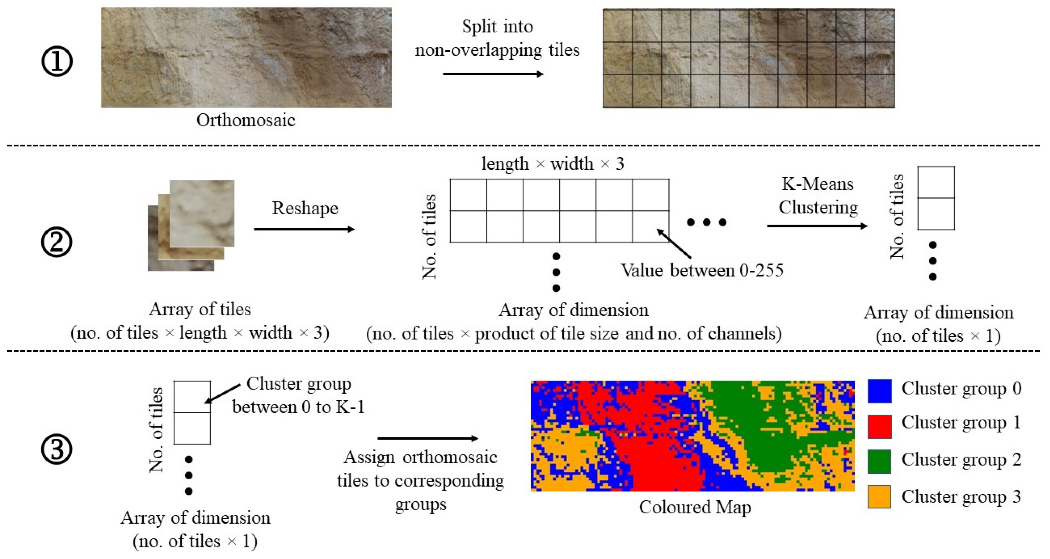
24]. For many ML algorithms, extensive and proper data labelling is extremely important. Given that it is frequently time-consuming and tedious, alternative solutions such as unsupervised learning methods may help alleviate this issue. These methods include different clustering algorithms, such as K-Means clustering [25,
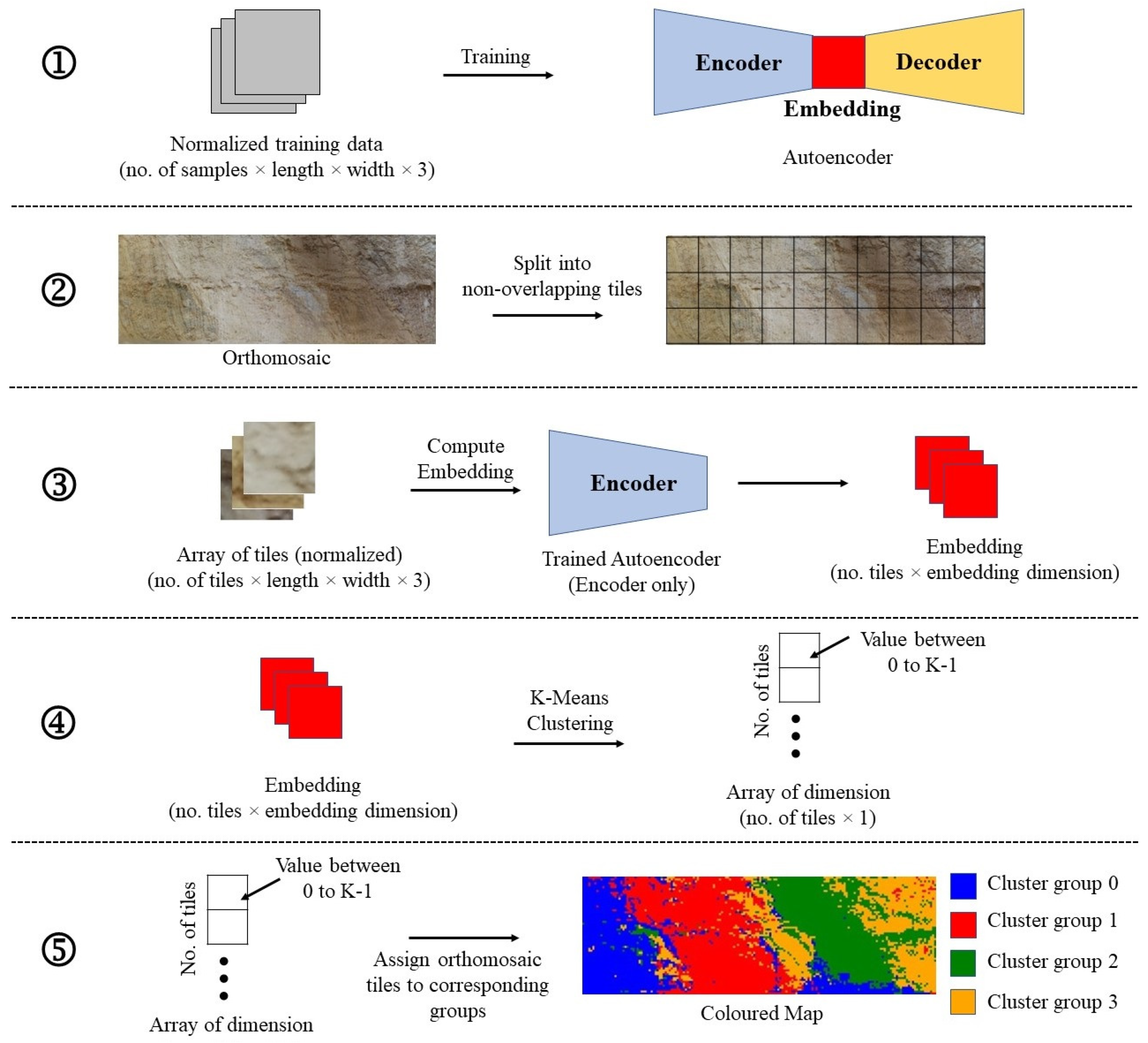
26], as well as an unsupervised DL approach called autoencoders. The concept of combining autoencoders with clustering algorithms has recently drawn increased interest, with many studies using DL architectures and traditional clustering techniques [27,28,29,30]. However, its use for geological and mining applications has not been well studied.
This study investigates using UAV-acquired RGB pit wall images and unsupervised learning algorithms to map different geological units of small pit wall sections in two mine sites. In particular, the algorithms are used to investigate their potential for geological pit wall mapping when there is an absence of ground truth information. The outcome of this work can form a basis for comparing results obtained through other remote sensing techniques, ML algorithms, and data types.

2. Materials and Methods

2.1. Study Sites

Kinross Gold’s Bald Mountain mine (39°56′N, 115°36′W, WGS 84) is a gold-producing mine operation located south of Elko, Nevada, within the Carlin Trend. A unique feature of Bald Mountain is the presence of multiple pits. These pits are generally smaller and more dispersed, which creates challenges when manually collecting geological data. The local geology is diverse and complex, with mineralization occurring in multiple large-scale faults, different rock formations such as intrusive and sedimentary rocks, and alterations. In general, deposits in the northwest are more structurally controlled and hosted in carbonate rocks and intrusive rocks, while deposits in the east and south are more stratiform and hosted by siltstones and sandstones. Gold mineralization is hosted in a thick sequence of chemical and siliciclastic sediments. The pit where data were collected is called Top Pit, which consists of Cambrian Dunderberg siltstones, Cambrian Windfall Hornfels/Marble, Ordovician Pogonip limestones, and Jurassic felsic intrusions in different alteration conditions, as well as the presence of a major fault.
McEwen Mining’s Gold Bar mine (39°47′N, 116°20′W, WGS 84) is also a gold mine located near Elko, Nevada, relatively close to Bald Mountain, but despite the proximity, the site geology and mineralization are very different. The ore deposits occur in thin-bedded carbonate rocks, with mineralizations localized by structural conduits that trend northwest and northeast. In general, the ores are mainly sulphide or oxide-dominant and located in carbonate rocks and mixed with various clay-dominated alterations. The three ore types are oxidized, jasperoidal, and carbonaceous ores, with the latter two predominantly associated with sulphides. Data were collected in Gold Bar’s Pick Pit, and they mainly consist of sedimentary rock formations including McColley Canyon Formation and Denay Formation, with different types and degree of alterations. Figure 1 shows the location of the two mine sites.

2.2. UAV Equipment

The DJI Inspire 2 UAV (DJI, Shenzhen, China) with high altitude propellers and its default camera system Zenmuse X5S (DJI, Shenzhen, China) was used for image acquisition. The Zenmuse X5S is a 20.8 MP camera with a 5280 × 3956 pixels resolution. Special propellers were used to improve performance and reduce battery consumption since the mine sites were located at least 2000 m above sea level. The default 15 mm f/1.7 ASPH lens was used in addition to the Olympus M.Zuiko 45 mm/1.8 lens (OM Digital Solutions, Tokyo, Japan) with a balancing ring. Focal length refers to the distance between the lens and a point of focus, and the use of the longer focal length lens was to increase image details through enlargement at the expense of a narrower field of view [31,32]. This is particularly important for detailed pit wall mapping since the minute details on the walls can be captured at high magnification and resolution. The default lens provides an angle of view of 72° while the Olympus lens is 27°. The Inspire 2 was selected due to its simple setup and fast battery recharge speed, and the entire UAV system setup has been successfully used in previous experiments for collecting other data including structural features of pit walls [33,34]. Additionally, the DJI Ground Station Pro application (DJI GS Pro) was used for planning and executing flight missions. All the equipment was used in an identical fashion at both mine sites.

2.3. Data Acquisition

There are very limited guidelines for UAV flight planning for mining purposes, and poor planning can negatively affect the results [35]. In this study, the UAV data collection process, including flight plan design, was based on guidelines outlined in Bamford et al. [33]. The entire process is divided into two phases. The first phase was coarse topographic mapping of the selected pit wall area, and the second phase was the detailed mapping of pit walls.

2.3.1. First Phase: Coarse Topographic Mapping

The first phase in the pit wall image data collection process is to perform a topographic mapping of the area of interest (i.e., the section of the pit to be mapped) to create a digital elevation model (DEM), which is required for the second phase’s flight mission planning. If a georeferenced DEM is available and accurate, then this first phase can be skipped entirely; however, it is still best to conduct this first phase if time permits since the DEM created will be the most up-to-date. Although Bald Mountain and Gold Bar had DEMs available, the coordinate systems differed from the WGS 84 coordinate reference system used in DJI products. While coordinate transformation is technically possible, converting from local mine grid coordinate systems can be time-consuming and tedious.
Coarse topographic mapping at the mine sites started with flying the UAV to the boundaries of the area of interest and recording its positions on the DJI GS Pro to form a polygon containing the pit wall of interest. Then, a flight plan was created where the UAV captured images from a top-down view covering the polygonal area in a “lawnmower” style. Since the required resolution can be coarse, the flight height can be set to the maximum allowable height to reduce flight time and subsequent image processing time, and the default lens can be used. After the images were captured, photogrammetry was used to generate the DEM.

2.3.2. Second Phase: Detailed Pit Wall Mapping

After obtaining a DEM covering the area of interest, the second phase begins by creating a flight plan to capture detailed images of the pit wall. The flight parameters were determined by choosing the ground sample distance (GSD) and overlap, and then calculating the other flight parameters using the following equations [33,36]:
f v = 2 arctan tan A O V 2 2 H 2 V 2 + 1
f h = 2 arctan ( tan ( f v 2 ) H V )      
z = G S D 2 i w i h 4 tan f h 2 tan f v 2
s = 2 z tan f h 2 1 o v e r l a p s i d e
f = 2 z tan f v 2 1 o v e r l a p f r o n t
v f = s t p
where fv and fh are the lens’ vertical and horizontal angle of view, respectively; AOV is the angular extent of the scene captured; H and V are the horizontal and vertical aspect ratio, respectively; z is the distance from the target; iw and ih are the camera image width and height, respectively; s and f are the side and front spacing between images, respectively; vf is the flight speed; and tp is the shutter interval (time delay between image captures).
Equations (1) and (2) calculate the camera lens’ angle of view in the horizontal and vertical direction, while Equation (3) gives the distance from the pit wall face. Using these results, the side and front spacing can be determined from Equations (4) and (5). Lastly, the flight speed was calculated from Equation (6).
The flight paths can be completely horizontal or vertical but must remain parallel to the pit wall and the camera perpendicular to the face to ensure constant GSD and good surface coverage. Determining the appropriate GSD value depends on the pit wall conditions and the data resolution, all of which should ideally be known beforehand, while the image overlap should be as high as practically possible but not below recommended ranges for photogrammetry [35,37]. Although there is not a minimum safe offset distance, sufficient contingency should be given in case of sudden wind gusts or mechanical issues to avoid collisions with the pit wall. The flight speed should ideally be as slow as possible to minimize image blur, but it needs to be adjusted based on the camera shutter interval, flight time, and battery availability. Since DJI GS Pro only supports a limited number of shutter intervals, it is selected beforehand to calculate flight speed.
After calculating the flight parameters, the DEM was imported into QGIS (QGIS.ORG, Version 3.24) to create contour lines at an interval equal to the front spacing. These lines are effectively the UAV flight paths during data collection. After only keeping the lines pertinent to the section of the pit wall, they were slightly adjusted to ensure a smooth flight while maintaining a constant offset distance and pit wall perpendicularity as best as possible. These lines were horizontally offset from the wall by a distance equal to the offset distance and annotated with their respective altitudes. Finally, the flight paths were imported into DJI GS Pro (DJI, Shenzhen, China), each corresponding to its own flight mission. Each mission’s parameters were manually set, and its starting point corresponds to the ending point of the previous mission. The mapped pit wall sections are shown in Figure 2, and the calculated flight parameters and mission details are presented in Table 1.

2.4. Photogrammetry

After acquiring pit wall images, they were used to generate a 3D point cloud model and orthomosaics using the Agisoft Metashape software (Agisoft, St. Petersburg, Russia, Version 1.6). In Agisoft’s photogrammetric workflow, all default settings were used with both photo alignment accuracy and dense point cloud quality set to high. Figure 3 shows the point clouds of Top Pit and Pick Pit. For georeferencing, only the EXIF information stored in the image files was used, and no ground control points (GCPs) were added. It is best practice to use GCPs to ensure that the point clouds are properly aligned as GPS information may not always be reliable; however, given the time constraint and inaccessibility to the upper pit wall benches, GCPs were not used. Although some prisms were placed on the walls, they were too small to be identified on the point clouds.
Figure 3b shows that the model for Pick Pit contains many missing areas and extreme lighting differentiation. There is a whitening effect caused by overexposure on the left side, while the right side is slightly underexposed despite adjusting camera parameters in real-time and having all the images captured around 10 AM local time within a span of an hour. Amongst the “holes” in the point cloud, a significant portion of the circular enclave is missing due to the lack of images and insufficient overlap in that area. Since a constant offset distance from the pit wall was required at all times during the flight, it was not possible for the UAV to do so in the circular enclave without colliding with the pit wall behind it. Attempts to capture images of the enclave at a much smaller offset distance were unsuccessful due to possible collisions with the tall drilling equipment in the area and poor weather conditions. This enclave poses a challenge using the detailed pit wall mapping method outlined earlier since a separate flight plan is required at a much smaller GSD. The significant and abrupt difference in GSD may impact the quality of the point cloud model if images captured from both flights are all used for the same model. Alternatively, separate point clouds can be created at the loss of having one model covering the entire area. It may also be possible to create flight plan(s) that gradually increase or decrease offset distance for a gradual change in GSD. Additionally, the presence of tall structures and equipment may increase the risk of collision when the UAV is mapping the lower parts of the pit wall.

2.5. Dataset Creation for Unsupervised Learning

By visually observing the 3D point cloud model for Top Pit, a small area of a bench with distinct and simple colour separation (Figure 3a) was identified and selected since colour is intuitively the main feature observed in images. A 2D orthomosaic roughly perpendicular to the face was then created and trimmed to produce a 11,273 × 3907-pixel raster image (Figure 4a), corresponding to a 70.6 × 24.5 m area at a GSD of approximately 0.626 cm/pixel. A “novice-labelled” ground truth map (Figure 4b) was labelled by the author using a rough sketch of the lithological boundaries provided by an onsite geologist; however, it was not used during the analyses and only after the results were produced for qualitative and quantitative assessments. The main lithologies present in the selected section are the Cambrian Windfall formation, Jurassic Granodiorite Intrusive, and Ordovician Pogonip (Figure 4b). The Windfall here consists of West Top Fault gouge and breccia heterolithic clasts, mostly just Windfall clasts. The intrusive has been differentially altered into two distinct sections, so despite being the same unit, they were separately classified into weakly and moderately oxidized Intrusives. Based on the information provided by the onsite geologist, the Pogonip in this area is difficult to differentiate from the Windfall, meaning that both interpretations would be considered acceptable, and so the Pogonip was used as the lithological class. Using these interpretations, the ground truth map consists of four classes, and the Top Pit dataset is considered as the “simple case”.
Similar to Top Pit, a bench was selected for analysis by visually observing the 3D point cloud model of Pick Pit (Figure 3b), and a 12,118 × 3371-pixel orthomosaic was produced (Figure 5a). At a GSD of around 0.574 cm/pixel, this area is 69.6 m × 19.3 m. The geology in this section of the Pick pit is more complicated than the simple case selected for Top Pit. One key difference between the Top Pit data and the Pick Pit data is the geology identified and predicted. For Top Pit, multiple lithologies were exposed on the selected pit wall section, while the only lithology present in the Pick Pit orthomosaic is limestone. The limestone is largely unaltered with varying degrees of alterations that are mainly distinguished by characteristic colours; therefore, this dataset targets the alterations rather than the lithologies. The “novice-labelled” ground truth map was also labelled by the author using a general sketch of the alteration boundaries from an onsite geologist as guidance (Figure 5b). This time, the labelling task was challenging due to the complex spatial distribution of the alterations. Despite only establishing three classes in total, in reality, they are not distinct and homogeneous throughout this section of the pit wall, and class definition is highly subjective. The altered regions contain at least two types of alterations of different intensities, but unaltered limestones occur intermittently throughout. The labelling was done to simplify the ground truth by assignment based on the most visually prominent alteration. The unaltered sections were grouped into classes depending on the surrounding alteration type. These decisions made during geological data labelling profoundly impact qualitative and quantitative assessments of the generated maps, and discussions on them will be made later when presenting the results. The Pick Pit dataset is considered as the “complex case”.
To create the input data for the unsupervised learning algorithms, the orthomosaics were separately divided into five non-overlapping tile sets of different sizes ranging from 64 to 256 pixels. Since the orthomosaic is 8-bit, each colour channel has a minimum and maximum possible value of 0 and 255, respectively. Due to the larger dimensions, the number of tiles in the 192 × 192 and 256 × 256 datasets was significantly smaller, so data augmentation was used to increase the tile count closer to that of 128 × 128 tiles. To increase the number of tiles, additional tiles were randomly cropped from tiles of 384 × 384 pixels. Table 2 and Table 3 summarize the number of tiles generated for each tile dimension in the Top Pit and Pick Pit, respectively.

2.6. Unsupervised Learning Algorithms and Cluster Map Generation

This study used two unsupervised learning approaches: a K-Means clustering approach and an autoencoder-first K-Means clustering approach. Image data tiles were clustered using K-Means clustering to generate a map indicating regions clustered together; however, the latter approach first utilized a trained autoencoder to produce an embedding of each tile instead of clustering the original tiles; and the embedding versions were used. The embeddings should represent a lower-dimensional space learned by the autoencoder that will improve clustering results by only including important features derived from the original data. Ideally, each cluster group should correspond to a specific geological unit. Since the different tiles are grouped into different clusters, they essentially represent the smallest area covered by a specific unit. Segmentation was also done as a simple visual comparison to the classification approach.

2.6.1. K-Means Clustering

K-Means clustering was conducted using scikit-learn in Python with all default parameters, but the random state parameter was set to an integer value of 1, which ensured that centroid initialization was consistent across all data. The map generation process is depicted in Figure 6 and started with splitting the orthomosaic into non-overlapping tiles of a specified size and then clustering using K-Means. Any tiles that were not of the required size were removed, which corresponded to the right and bottom edges of the orthomosaic. K was set to the number of classes defined in the ground truth, and the input data dimension was the number of tiles × product of the tile size and the number of colour channels. After being assigned a cluster group, a map was generated using the tiles and coloured based on the cluster group number.

2.6.2. Autoencoder-First K-Means Clustering

Autoencoders are neural networks that learn to produce a copy of the input as the output using an encoder-decoder architecture and are generally used for dimensionality reduction or feature learning but have seen uses in generative models in more recent times [38]. In general, the encoder portion of an autoencoder produces a code or embedding that is used by the decoder to reconstruct the input. The idea is that through training the autoencoder, it will learn useful features and represent them in the embedding layer that usually has a smaller dimension than the input [38]. These embeddings will then be used as input into a clustering algorithm, e.g., K-Means, as opposed to the original data. In the approach described in this section, the autoencoder was first trained from scratch using data prepared as described in Section 2.5, which were also normalized by the mean and standard deviation of each channel. Then, a map was generated based on the original orthomosaic by applying K-Means clustering on the embeddings produced by the encoder (Figure 7).
The autoencoders used consisted mainly of convolutional layers (i.e., down-sampling and up-sampling were done using convolutional layers) with a fully-connected layer in both the encoder and decoder to produce and unpack the embedding layer. Two slightly different architectures were used where the first one (Model MT) was slightly asymmetrical with a smaller decoder while the second one (Model PY) was completely symmetrical. This was to observe and to explore any differences in the results between the two slightly different architectures. Although autoencoders are generally symmetrical, it is not a requirement for architectural design, and asymmetry can show improvements over symmetrical counterparts [39,40,41]. Model MT and Model PY each has 1.6–17.5 M parameters and 2.1–17.9 M parameters, respectively, for tile sizes ranging from 64 × 64–256 × 256. The two architectures are summarized in Table 4 and Table 5. It should be noted that while both the encoder and decoder are required during training, only the encoder extracts features from the input data. Once model training has been completed, the decoder is not needed.
Implementation was conducted using PyTorch with all models trained from scratch. Mean squared error (MSE) was used as the loss function since it is typically used in autoencoders [38]. The Adam optimizer [42] with default settings was used at a learning rate of 0.001. Network parameters were initialized through Kaiming initialization [43], and the training data were randomly shuffled before training. The main hyperparameters adjusted during the training process were batch size and epoch in both architectures for different input tile dimensions, as shown in Table 6 for Top Pit and Pick Pit datasets. The batch size was set to as large as computationally possible while training was stopped when the loss did not change substantially. The number of features for each embedding was set as 128. A comparison of results at different training stopping points after a noticeable plateau in the training curve was made with no appreciable differences. Autoencoder training by far required the greatest computational time of up to 60 min for 256 × 256 tiles while the actual clustering and map generation process generally took less than 5 min.

2.6.3. Segmentation

Using the ESRI ArcMap software’s built-in ISO Cluster Unsupervised Classification tool, segmentation (Version 10.7) was done on the Top Pit and Pick Pit orthomosaics. This tool combines ArcMap’s ISO Cluster tool and Maximum Likelihood Classification tool to perform clustering and classification all in one step. Other than the maximum number of classes being set to the number of classes defined in the ground truth, the other inputs were left as the default values.

3. Results

3.1. Top Pit

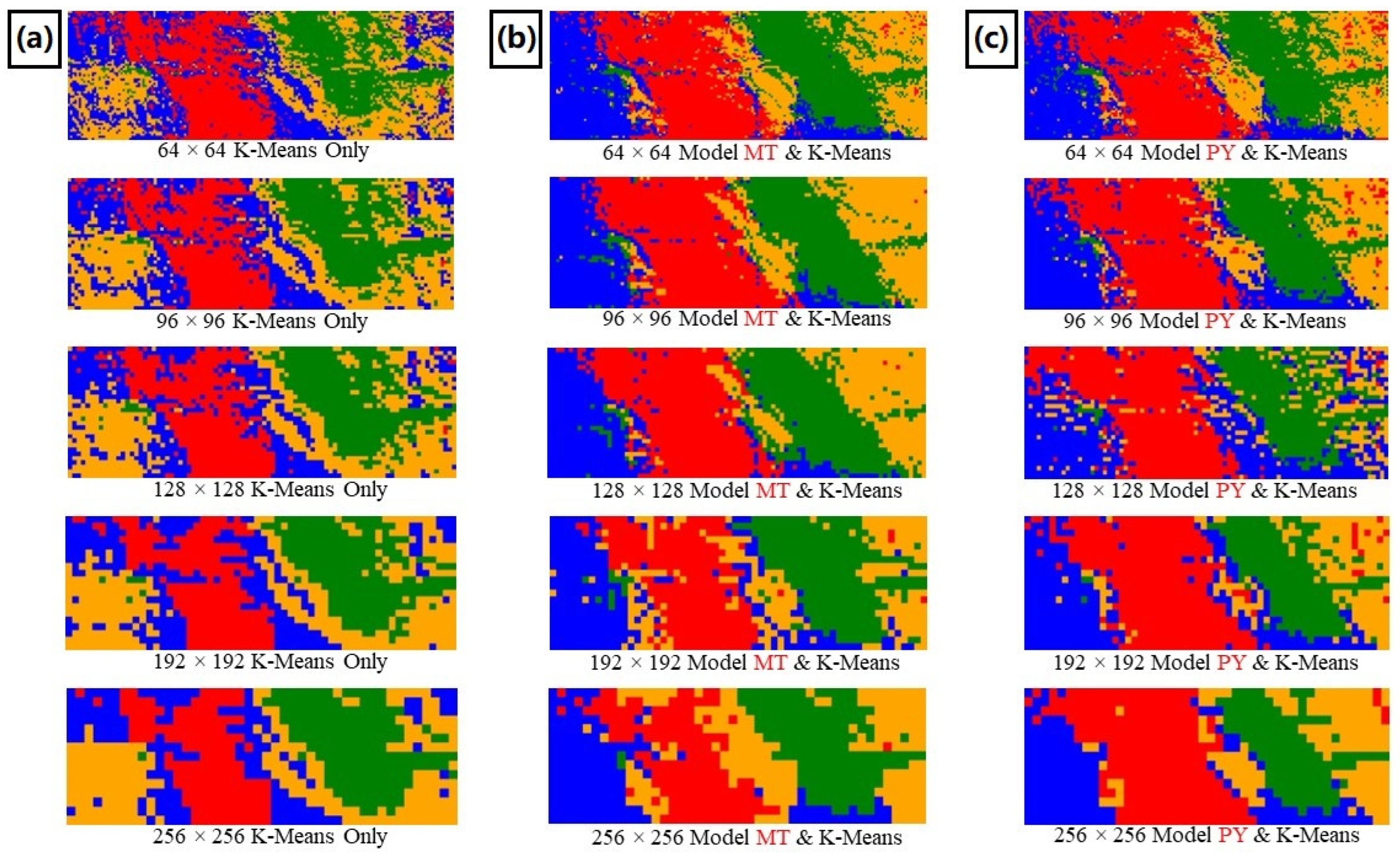
Figure 8 shows the generated maps using the K-Means clustering approach and the autoencoder-first K-Means clustering approaches. To complement the qualitative assessment, tile accuracies (Table 7) and F1 scores (Table 8) were calculated to provide some numerical metrics. Tile accuracy is defined as the percentage of correctly clustered tiles compared to the ground truth. This involves converting the ground truth map from pixel-level resolution to tile-level resolution. For the ground truth map, if a tile contained pixels from different classes, the class with the most pixels was assigned to the whole tile.
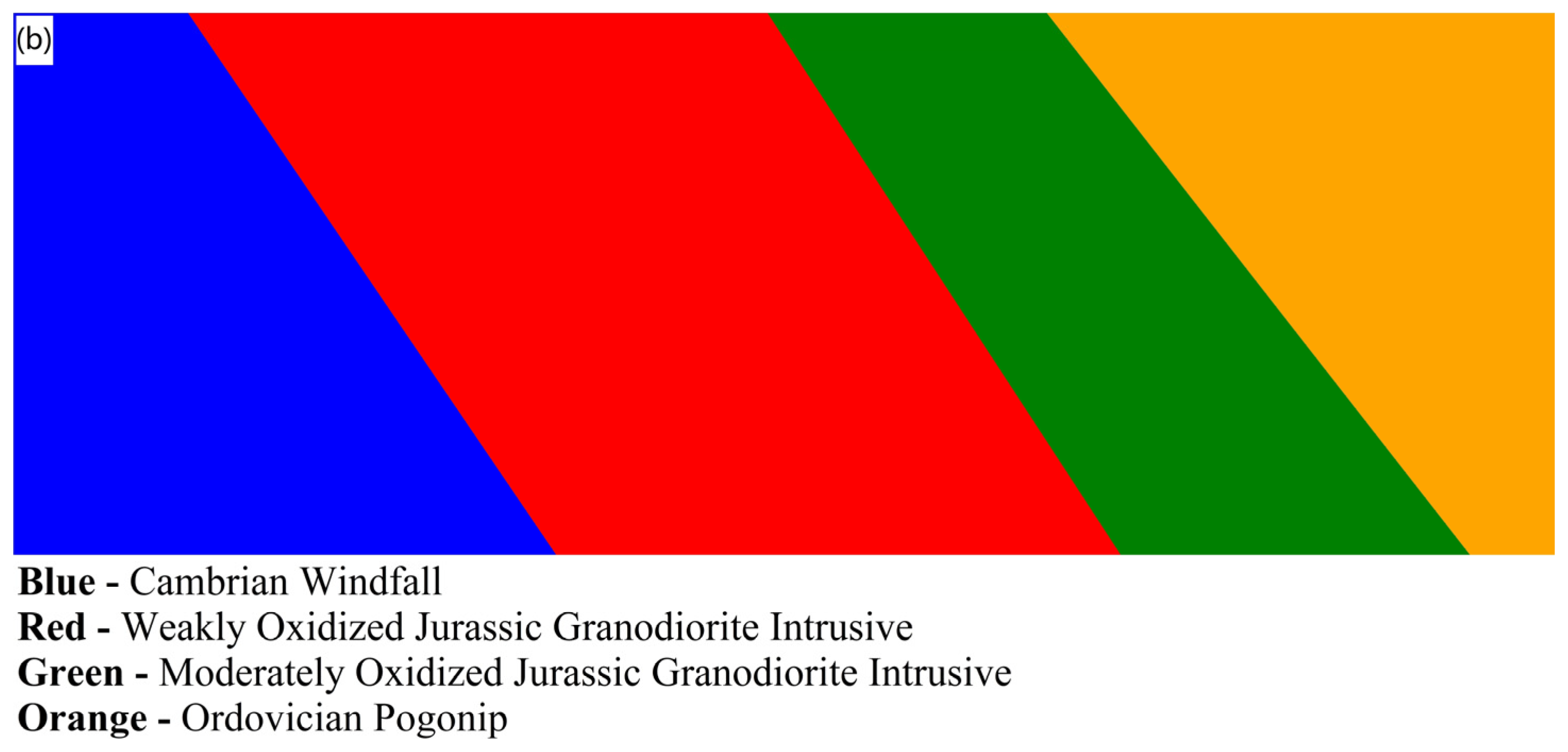
The results between the two unsupervised learning approaches are visually comparable to each other and the ground truth in Figure 4b, particularly between the outputs of the two autoencoder architectures. However, based on accuracy and F1 scores, it is clear that K-Means clustering by itself does not perform as well. Cambrian Windfall (blue) and Ordovician Pogonip (orange) predictions are much better across all tile dimensions when the encoder embeddings are clustered instead of the original tiles. The maps for different tile dimensions are nearly identical within the K-Means clustering-only results. This suggests that even the smallest tile dimension used is too large for this clustering-only approach due to the high data dimensions when clustering.
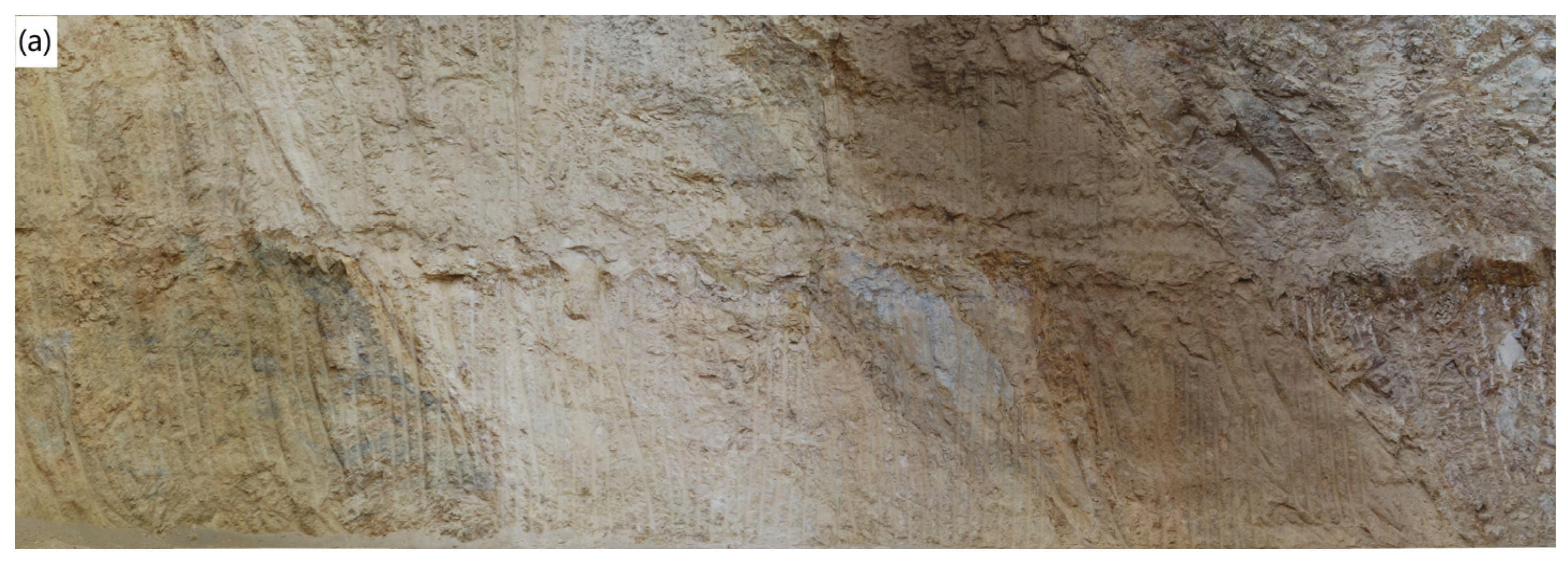
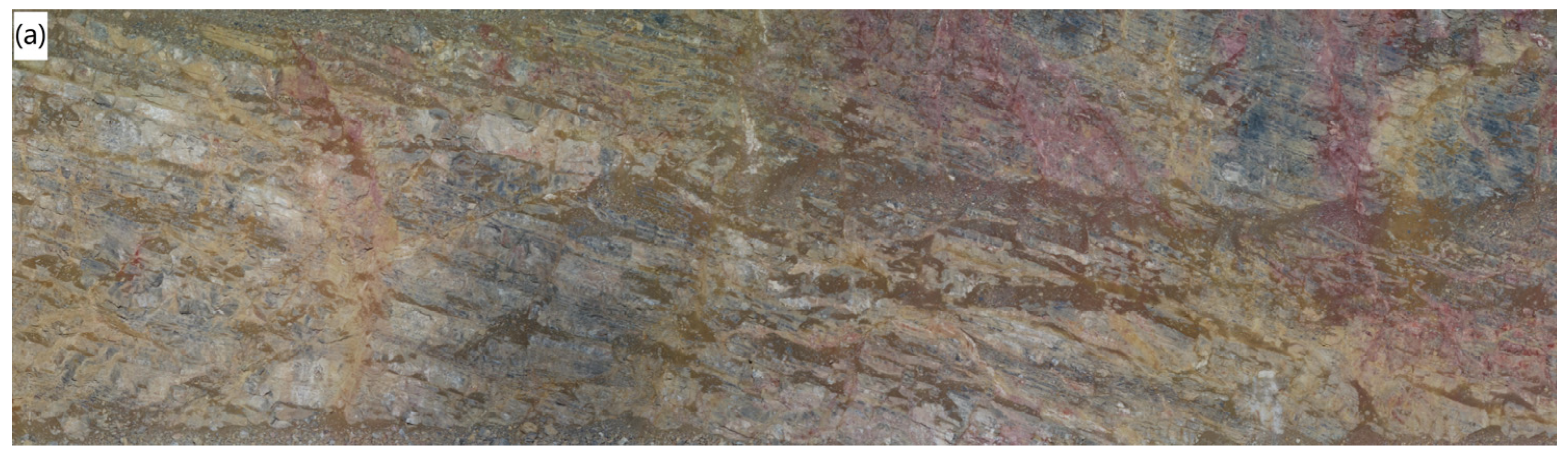
The weakly oxidized Intrusive (red) and moderately oxidized Intrusive (green) match closely across all results, while differences occur primarily in the Cambrian Windfall (blue) and Ordovician Pogonip (orange). From observing the orthomosaic (Figure 4a), weakly oxidized Intrusive and moderately oxidized Intrusive represent areas of more uniform colouring than Cambrian Windfall and Ordovician Pogonip. This is the most apparent for Ordovician Pogonip, where colour differentials are the most extreme. Additionally, a grey area between weakly oxidized Intrusive and moderately oxidized Intrusive was labelled as the former in the ground truth map but clustered with Ordovician Pogonip in all the results. This is likely due to the presence of grey-coloured regions in the Pogonip. This also occurs near the lower boundary between the Cambrian Windfall and Weakly oxidized Intrusive to a lesser extent. These observations suggest that colour is the main feature for clustering as expected.
For the maps generated using only K-Means, the Cambrian Windfall region is separated into two parts: the bottom portion is clustered with the Pogonip, and the boundary between the weakly oxidized Intrusive and moderately oxidized Intrusive are clustered with the Cambrian Windfall and Pogonip. The maps generated using autoencoder-based K-Means also exhibit the latter but to a much lesser degree. In the orthomosaic, these regions correspond to different shades of the same colour, which may indicate that the degree of shading plays a role in prediction; however, using an autoencoder makes the model more robust to slight changes in shading.
In the middle of the maps for the weakly oxidized Intrusive region, there is a tiny part that has been clustered as a different class, and this is slightly more apparent at smaller tile dimensions. Looking at the orthomosaic (Figure 4a), this corresponds to shadows caused by the rough textures, which shows that lighting condition has a significant effect. Still, it is slightly reduced when tiles increase in size. This is perhaps because the increasing number of surrounding normal pixels is “covering up the shadows”. In other words, as the number of pixels in each tile increases, the less percentage of the “shadow” pixels are present in the tile, thereby decreasing their influence on the clustering process. Note that this is not the case for the Pogonips because the middle part is actually of similar colour to the moderately oxidized Intrusive.
The results of the two autoencoder architectures are very similar except for the 128 × 128 tiled map for Model PY, which shows significantly higher predictions of Cambrian Windfall. This is mainly due to how the algorithms’ parameters were initialized because the convergence point can differ depending on the starting parameter values. Model PY produces slightly better results at 192 × 192 and 256 × 256 tile dimensions since Model MT erroneously predicted many weakly oxidized Intrusive and moderately oxidized Intrusive areas as Pogonip. Overall, given the simpler spatial distribution of the geology, the coarser resolutions do not appreciably deter visual interpretation of the maps. The lithological units’ boundaries are also somewhat consistent with the ground truth.
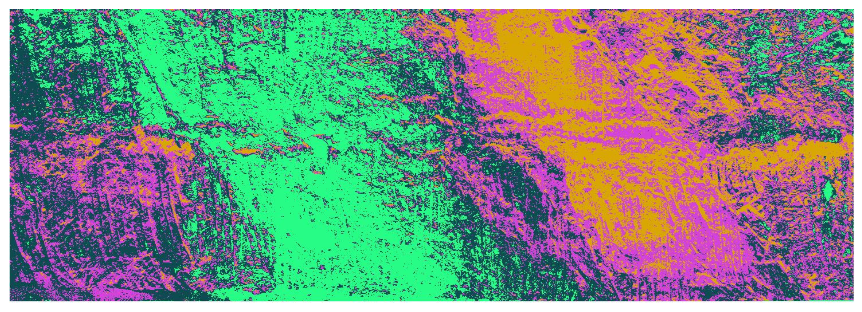
Lastly, the segmentation result in Figure 9 is reminiscent of the K-Means clustering-only results but with very fine resolution. One notable difference is the vertical streaks across the map, mainly shown in black colour, which were not present in the classification results. While these may suggest some type of structural pattern, they are more likely scratch marks left by shovel claws during excavations. This type of scenario not only deters from the visual clarity of the maps but can also be misleading, so caution should be exerted when making interpretations.

3.2. Pick Pit

Tile accuracies and F1 scores are listed in Table 9 and Table 10, respectively, for Pick pit. 
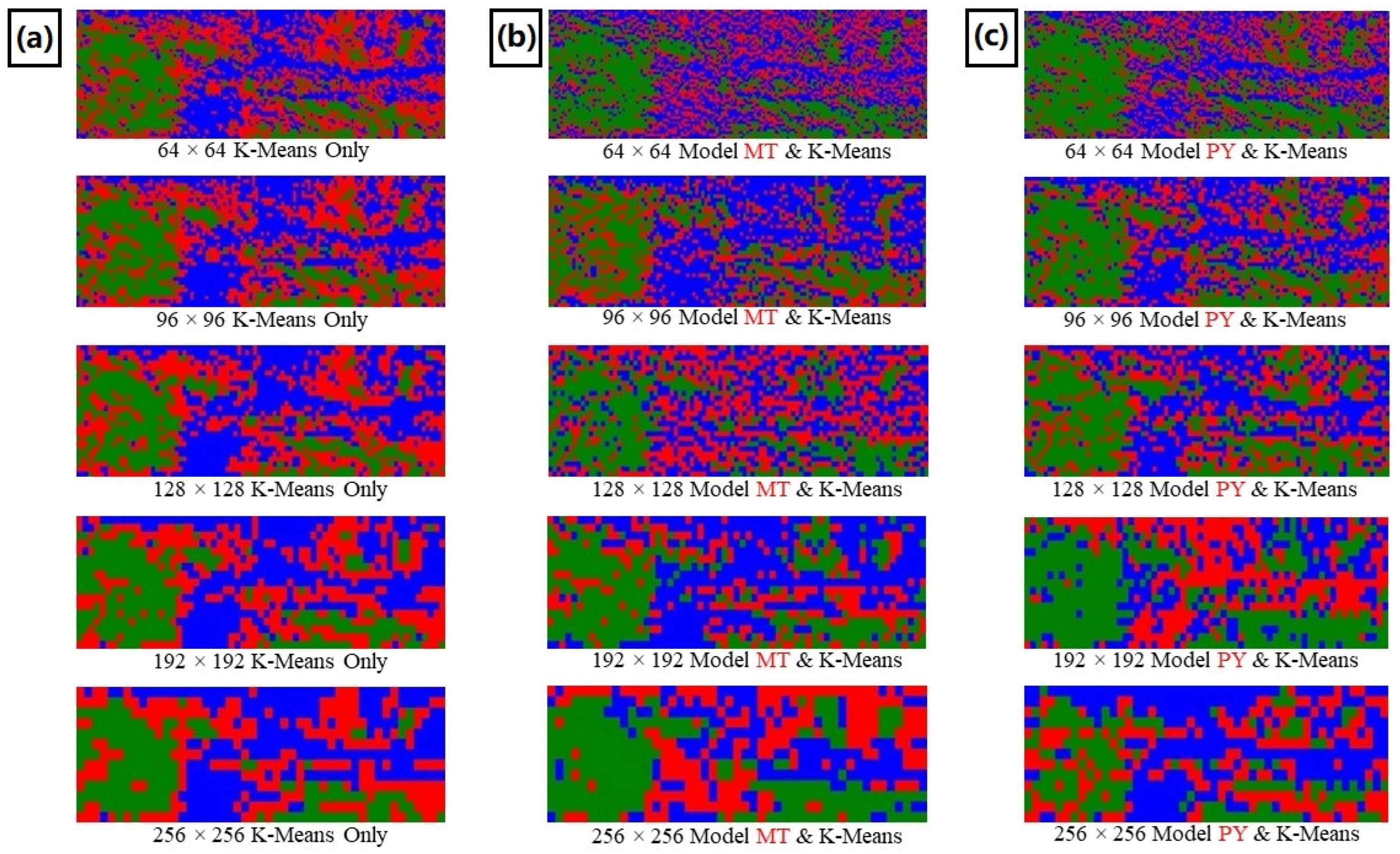
Figure 10 shows the generated maps using the K-Means clustering-only approach and the autoencoder-first K-Means clustering approaches.
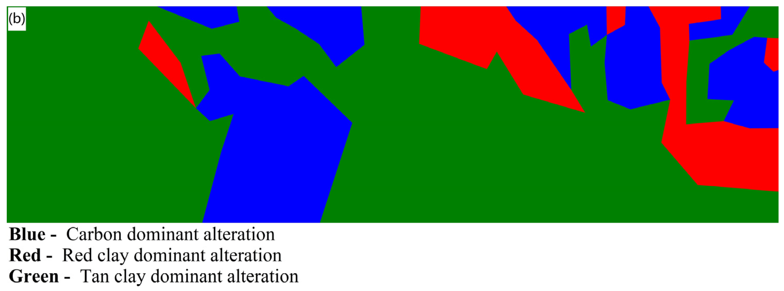
Looking at the results of K-Means clustering-only and the autoencoder-first K-Means clustering, it is apparent that interpretation is not as trivial as Top Pit, particularly due to the noise-like appearance in many areas, which could be the clustering algorithm’s forced attempt at identifying the user-specified number of clusters. Regardless of the method, all maps look different from the ground truth (Figure 5b) but have many similarities amongst each other. Assigning colours representing the different alteration classes to the cluster groups was difficult due to the stark contrast and large disagreements; hence, the maps do not look nearly as representative of the in situ conditions as the case for Top Pit.
For the tan clay-dominant alteration (green), most of it occurs on the left side and some in the bottom parts of the maps; however, based on the ground truth, it should cover most of the area on the right side as well. Instead, the carbon-dominant alteration (blue) covers large parts of it in each map with a seemingly horizontal orientation. Compared to the orthomosaic (Figure 5a), this seems to correspond to the dark brown streaks, especially the two large ones stretching from the middle to the right section of the orthomosaic. Based on the information provided by an onsite geologist, much of the tan clay is structurally controlled and thereby could suggest that the streaks are tan clay-dominant alterations or some type of joint filling, but in this case, the streaks are simply dirt or mud produced during mining operations.
The assigned cluster group for the red clay dominant alteration (red) does not correspond to the alteration itself. Many of the regions clustered together do not contain substantial traces of red clay, if at all. For this case, the assignment was only done to be consistent when interpreting the cluster groups as one cluster for each alteration class. In what was labelled as red clay in the ground truth, most, if not all, were considered as carbon- dominant alteration in the generated maps. In general, what was assigned as red clay could be areas representing a mixture of dark and light colours at most since this frequently occurs near boundaries of abrupt colour transitions. In some of the red clay pockets around the tan clay areas, this phenomenon could even represent the tan clay-dominant alteration enclosing the unaltered limestone.
The numerical results further support the poor representation of the alterations by the cluster groups. Although using autoencoders did show slight improvement, they should be disregarded and treated indifferently due to the large disagreements with the ground truth, especially between the red clay alteration and its corresponding cluster group. Visually speaking, it is difficult to say which method and tile dimensions were the best if there is one. K-Means clustering produced largely the same kind of results, something observed for Top Pit as well, while the two autoencoder architectures mainly differed at the larger tile dimensions. In particular, for Model PY’s 192 × 192 tile size map and Model MT’s 256 × 256 tile size map, the tiles were more distributed between the three cluster groups, which increased the tile accuracies. This is extremely misleading because the disagreement with the ground truth is so severe that it is difficult to say which cluster group corresponds to which alteration group. In turn, better quantitative metrics may not indicate improved model performance and could just be mainly based on a poor and forced decision of cluster-alteration assignment.
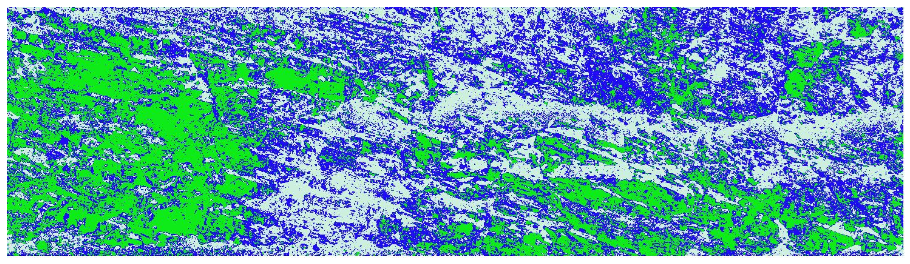
The segmentation result in Figure 11 shows some noticeable differences from the classification approach, with a few similarities to that of the Top Pit segmentation. Firstly, there is clearly some type of structure outlined by the white colour, including the dark brown streaks previously mentioned. So, unlike Top Pit, this pattern is more likely to correspond to rock structure. Secondly, the green colour appears to represent the unaltered limestone exposed on the wall surface and a bit of surficial calcite. The red clay is, however, not identified as its own group. Despite the finer resolution and noisier appearance, segmentation does yield some useful structural information that was not captured prominently by the classification approaches.

4. Discussion

This study has some limitations and potential areas of concern using unsupervised learning. One of them is that the interpretation of the final product will ultimately rely on at least knowing some geological information, especially during the assessment. Even if the spatial distribution and boundaries are well-defined, the only way to determine if they accurately represent in situ conditions is to compare them with some form of ground truth or assessment criteria. In this study, additional context was required using some type of reference to interpret the cluster maps. Although the ground truth was labelled by a novice, it was still useful to assess the clustering outcome. However, to obtain the ground truth, manual intervention is required, raising the problem of human subjectivity. Unlike conventional labelling tasks where there are usually definitive answers, such as annotating animals versus cars, the same process for mining and geological projects is more complicated and leaves a plethora of room for discussion and interpretation. The decisions made during data labelling directly affect the outcome, and they differ from person to person, even amongst experts.
While unsupervised learning methods are useful in the absence of quality labelled data, they have not been fully explored for geological applications. Without proper optimization and transformation, the high-dimensional space of the data may not be suitable for clustering, as shown in the Pick Pit alteration maps. Outside of the simple situations such as the one represented by the Top Pit data, most in situ conditions are far from ideal and resemble the condition in the Pick Pit orthomosaic, where multiple units of similar colours are mixed together. The 2D geological maps also lack 3D spatial context, limiting their usefulness when integrating with 3D geological models.
For data collection, UAVs are limited to certain operational conditions and exceeding these ranges may result in poor data quality [33]. Some of these are impossible to manipulate, including environmental conditions, which become intrinsic factors that must always be considered when collecting data. Additionally, the data collection process conducted in this study is far from optimal and requires significant time and manual adjustments, especially when creating flight plans for detailed pit wall mapping, as shown in the case of the Pick Pit point cloud model. In sections of the pit wall with irregular geometry, poor flight planning can result in missing areas in the point cloud models due to insufficient images. Lastly, the lack of GCPs decreases the point clouds’ spatial accuracy. It directly affects their uses for subsequent analyses, but GCPs are difficult to place on pit walls due to accessibility issues. It is also difficult to place GCPs in the surrounding perimeter due to the same accessibility issues and operating machineries on the working bench and pit ramp. In point clouds generated without GCPs or some form of accurate georeference, there is a risk of severe inaccurate orientation and positioning that prevents any form of 3D work to be done on the model such as structural mapping of joints and fractures. This effectively makes the point clouds unusable. One workaround is to use UAV LiDAR to create LiDAR point clouds as a validation for the photogrammetric point clouds. Given that the two-point clouds are created differently (i.e., LiDAR point clouds are generally based on calculated distance from sensor to target while RGB photogrammetric point clouds are created mainly from image features and camera parameters), it is less likely that both models will have the exact same error, if any, and thereby provide a good way to locate any abnormalities. The downside is that both RGB and LiDAR data need to be captured, which will increase cost and time, especially if separate UAV systems or sensor swap out is required. However, it is possible to have dual gimbal UAV setups allowing for both RGB and LiDAR sensors to capture data on the same flight in addition to sensors that integrate LiDAR and RGB modules into one, such as the Zenmuse L1 (DJI, Shenzhen, China). Real-time (RTK) and post-processing kinematic (PPK) techniques can also be used as alternatives [34] including RTK UAVs. Regardless, it is always best to have GCPs for the highest accuracy.

5. Conclusions

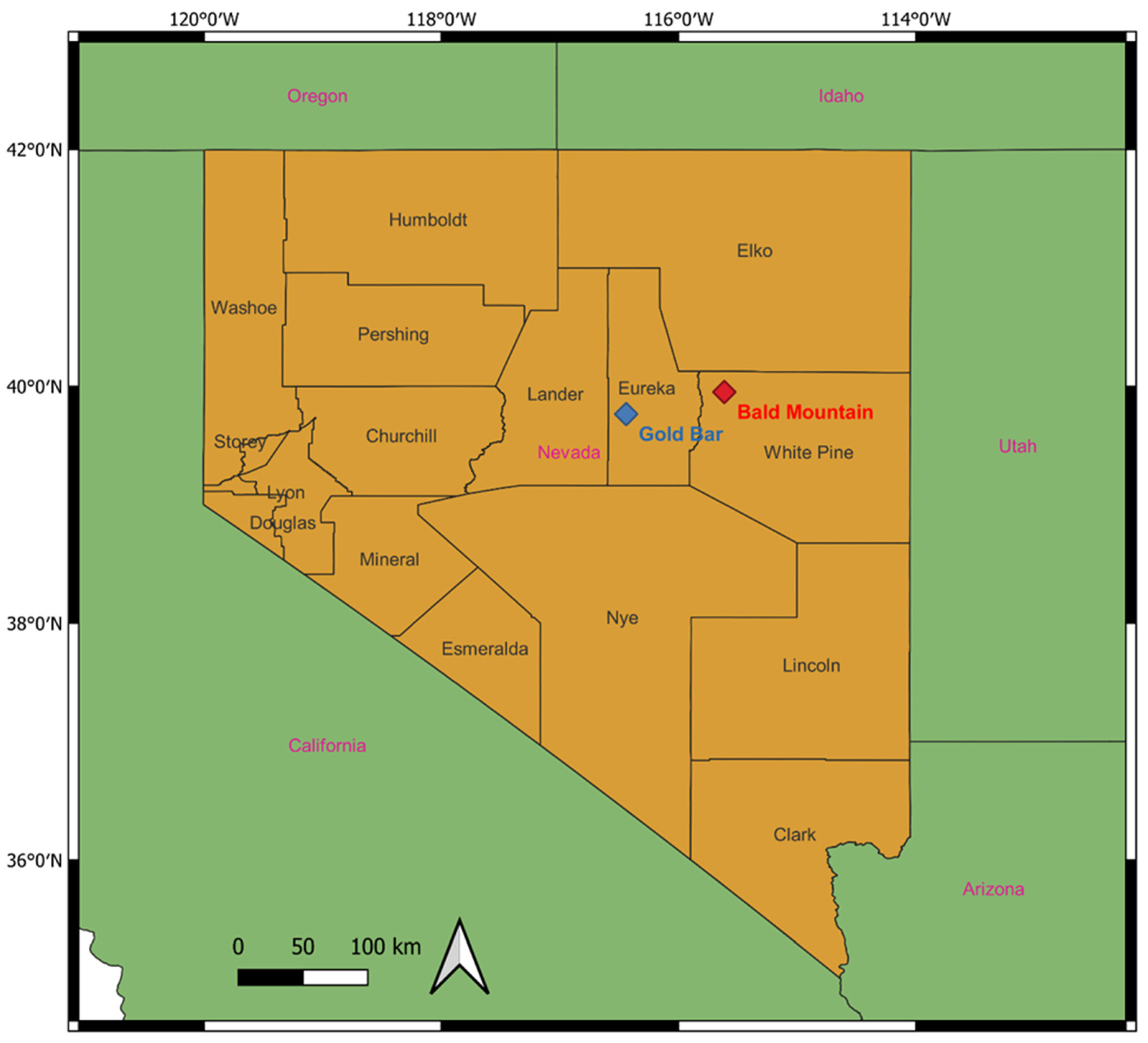
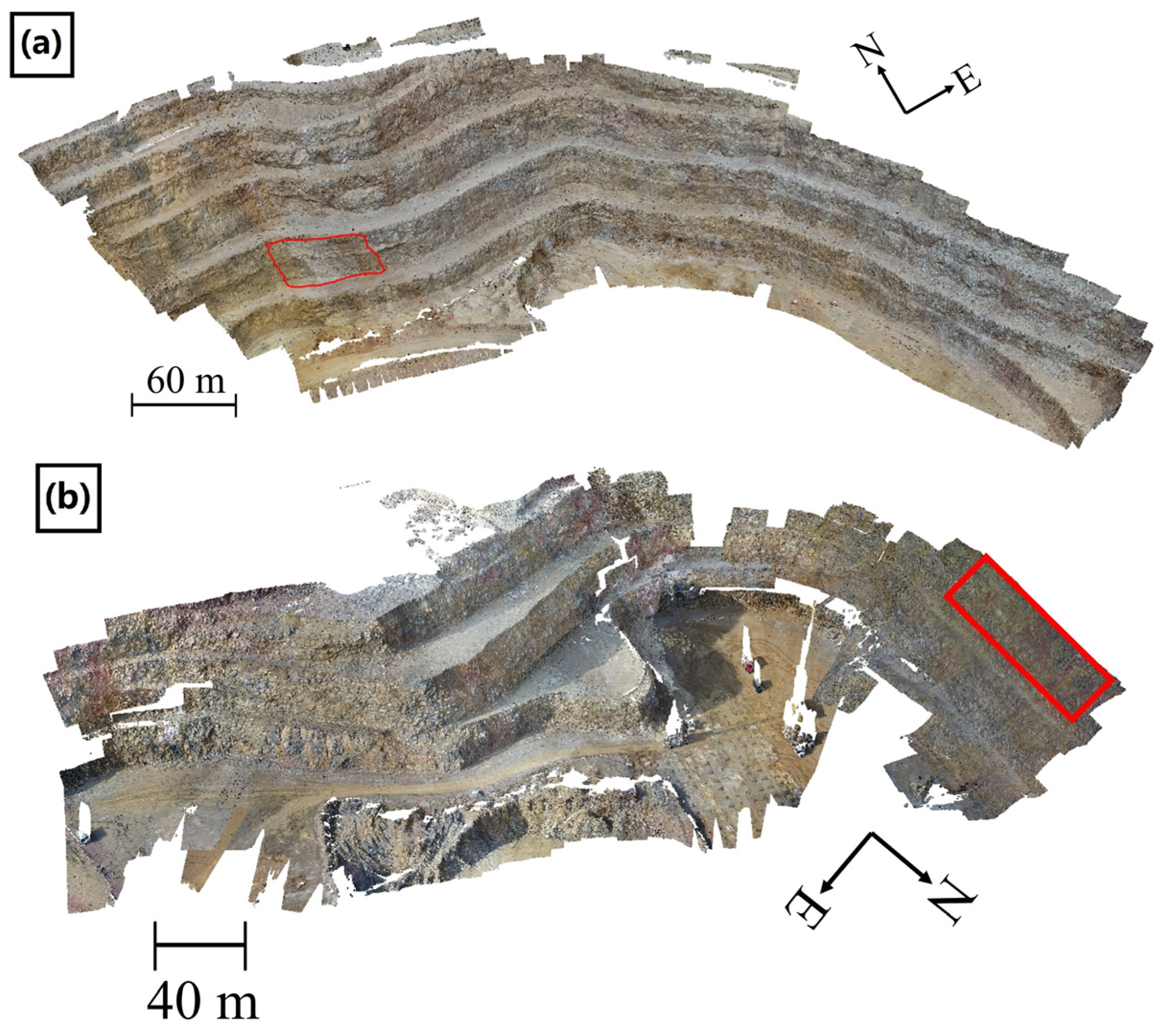
This study investigated using UAV-acquired RGB images and unsupervised learning algorithms for geological pit wall mapping. Using a commercial UAV, the high-resolution RGB images of pit walls were collected at Bald Mountain’s Top Pit and Gold Bar’s Pick Pit mine sites. Orthomosaics of the pit wall sections were then extracted from these point clouds as input data for clustering analysis and mapping of geological units in an unsupervised fashion. The Top Pit orthomosaic contained easily identifiable units and was designated as the simple case study, while the Pick Pit, with a more complicated geological spatial distribution, was used as the complex case study. In the simple case, the cluster groups corresponded well with the ground truth, but the clustering was not ideal in the more complicated case. Regardless, a better understanding of the application of UAV and RGB imaging for pit wall identification of surficial units in the absence of data labels was achieved.
Using two datasets with differing geology and complexity, a preliminary evaluation of identifying lithologies and alterations on pit wall surfaces demonstrated the challenges of using RGB images with unsupervised learning techniques. When colours are distinct, homogeneous, and directly correspondent to different geological units, the data type and techniques used are sufficient for lithological/alteration identification. In these cases, the resolution should primarily depend on the nature of work that will be done using information obtained from the maps. For mining operations, pit wall mapping is generally done at a relatively coarser scale. Usually, it corresponds to the block size of a block model, so a slightly coarser resolution should suffice. It is also dictated by the analytical techniques used to generate the maps. If too coarse, there may be an insufficient number of tiles for clustering and model training, while finer resolution may increase computational time due to the larger number of tiles or capturing unnecessary details.
Future works will investigate the use of semi-supervised learning by combining unsupervised and supervised DL models to reduce training time and the amount of data required. This approach can also be applied to data labelling to minimize labelling time and to reduce some model dependency on human inputs.

Author Contributions

Conceptualization, P.Y. and K.E.; methodology, P.Y., K.E., S.G. and J.C.O.C.; software, P.Y.; validation, P.Y., K.E., S.G. and J.C.O.C.; formal analysis, P.Y., K.E., S.G. and J.C.O.C.; investigation, P.Y., K.E., S.G. and J.C.O.C.; resources, K.E.; data curation, P.Y., K.E., S.G. and J.C.O.C.; writing—original draft preparation, P.Y.; writing—review and editing, K.E.; visualization, P.Y.; supervision, K.E.; project administration, K.E.; funding acquisition, K.E. All authors have read and agreed to the published version of the manuscript.

Funding

This research was funded by Natural Science and Engineering Research Council of Canada (NSERC), grant number ALLRP 560440-20.

Data Availability Statement

The data used are available from the corresponding author upon reasonable request with the permission of industry partners.

Acknowledgments

The authors would like to thank Kinross Gold Corporation and McEwen Mining Inc. for their financial and technical support.

Conflicts of Interest

The authors declare no conflict of interest.

References

  1. Blom, M.; Pearce, A.R.; Stuckey, P.J. Short-Term Planning for Open Pit Mines: A Review. Int. J. Min. Reclam. Environ. 2019, 33, 318–339. [Google Scholar] [CrossRef]
  2. Medinac, F.; Esmaeili, K. Integrating Unmanned Aerial Vehicle Photogrammetry in Design Compliance Audits and Structural Modelling of Pit Walls. In Proceedings of the 2020 International Symposium on Slope Stability in Open Pit Mining and Civil Engineering; Australian Centre for Geomechanics: Perth, Australia, 2020; pp. 1439–1454. [Google Scholar]
  3. McHugh, E.L.; Girard, J.M.; Denes, L.J. Simplified Hyperspectral Imaging for Improved Geologic Mapping of Mine Slopes. In Proceedings of the Third International Conference on Intelligent Processing and Manufacturing of Materials, Vancouver, BC, Canada, 20–23 August 2001; pp. 1–10. [Google Scholar]
  4. Van der Meer, F.D.; Van der Werff, H.M.; Van Ruitenbeek, F.J.; Hecker, C.A.; Bakker, W.H.; Noomen, M.F.; Woldai, T. Multi- and hyperspectral geologic remote sensing: A review. Int. J. Appl. Earth Obs. Geoinfo. 2012, 14, 112–128. [Google Scholar] [CrossRef]
  5. Murphy, R.; Schneider, S.; Monteiro, S. Mapping Layers of Clay in a Vertical Geological Surface Using Hyperspectral Imagery: Variability in Parameters of SWIR Absorption Features under Different Conditions of Illumination. Remote Sens. 2014, 6, 9104–9129. [Google Scholar] [CrossRef] [Green Version]
  6. Boubanga-Tombet, S.; Huot, A.; Vitins, I.; Heuberger, S.; Veuve, C.; Eisele, A.; Hewson, R.; Guyot, E.; Marcotte, F.; Chamberland, M. Thermal Infrared Hyperspectral Imaging for Mineralogy Mapping of a Mine Face. Remote Sens. 2018, 10, 1518. [Google Scholar] [CrossRef] [Green Version]
  7. James Fraser, S.; Whitbourn, L.B.; Yang, K.; Ramanaidou, E.; Connor, P.; Poropat, G.; Soole, P.; Mason, P.; Coward, D.; Philips, R. Mineralogical Face-Mapping Using Hyperspectral Scanning for Mine Mapping and Control. In Proceedings of the Sixth International Mining Geology Conference, Darwin, Australia, 23 August 2006; pp. 227–232. [Google Scholar]
  8. Buckley, S.; Kurz, T.; Schneider, D. The Benefits of Terrestrial Laser Scanning and Hyperspectral Data Fusion Products. In Proceedings of the International Archives of the Photogrammetry, Remote Sensing and Spatial Information Sciences, Melbourne, Australia, 25 August–1 September 2012; pp. 541–546. [Google Scholar]
  9. Murphy, R.J.; Taylor, Z.; Schneider, S.; Nieto, J. Mapping Clay Minerals in an Open-Pit Mine Using Hyperspectral and LiDAR Data. Eur. J. Remote Sens. 2015, 48, 511–526. [Google Scholar] [CrossRef]
  10. Murphy, R.J.; Monteiro, S.T. Mapping the Distribution of Ferric Iron Minerals on a Vertical Mine Face Using Derivative Analysis of Hyperspectral Imagery (430–970 nm). ISPRS J. Photogramm. Remote Sens. 2013, 75, 29–39. [Google Scholar] [CrossRef]
  11. Lorenz, S.; Salehi, S.; Kirsch, M.; Zimmermann, R.; Unger, G.; Vest Sørensen, E.; Gloaguen, R. Radiometric Correction and 3D Integration of Long-Range Ground-Based Hyperspectral Imagery for Mineral Exploration of Vertical Outcrops. Remote Sens. 2018, 10, 176. [Google Scholar] [CrossRef] [Green Version]
  12. Kirsch, M.; Lorenz, S.; Zimmermann, R.; Tusa, L.; Möckel, R.; Hödl, P.; Booysen, R.; Khodadadzadeh, M.; Gloaguen, R. Integration of Terrestrial and Drone-Borne Hyperspectral and Photogrammetric Sensing Methods for Exploration Mapping and Mining Monitoring. Remote Sens. 2018, 10, 1366. [Google Scholar] [CrossRef] [Green Version]
  13. Barton, I.F.; Gabriel, M.J.; Lyons-Baral, J.; Barton, M.D.; Duplessis, L.; Roberts, C. Extending Geometallurgy to the Mine Scale with Hyperspectral Imaging: A Pilot Study Using Drone- and Ground-Based Scanning. Min. Metall. Explor. 2021, 38, 799–818. [Google Scholar] [CrossRef]
  14. Thiele, S.T.; Lorenz, S.; Kirsch, M.; Cecilia Contreras Acosta, I.; Tusa, L.; Herrmann, E.; Möckel, R.; Gloaguen, R. Multi-Scale, Multi-Sensor Data Integration for Automated 3-D Geological Mapping. Ore Geol. Rev. 2021, 136, 104252. [Google Scholar] [CrossRef]
  15. Thiele, S.T.; Bnoulkacem, Z.; Lorenz, S.; Bordenave, A.; Menegoni, N.; Madriz, Y.; Dujoncquoy, E.; Gloaguen, R.; Kenter, J. Mineralogical Mapping with Accurately Corrected Shortwave Infrared Hyperspectral Data Acquired Obliquely from UAVs. Remote Sens. 2021, 14, 5. [Google Scholar] [CrossRef]
  16. Chesley, J.T.; Leier, A.L.; White, S.; Torres, R. Using Unmanned Aerial Vehicles and Structure-from-Motion Photogrammetry to Characterize Sedimentary Outcrops: An Example from the Morrison Formation, Utah, USA. Sediment. Geol. 2017, 354, 1–8. [Google Scholar] [CrossRef]
  17. Madjid, M.Y.A.; Vandeginste, V.; Hampson, G.; Jordan, C.J.; Booth, A.D. Drones in Carbonate Geology: Opportunities and Challenges, and Application in Diagenetic Dolomite Geobody Mapping. Mar. Pet. Geol. 2018, 91, 723–734. [Google Scholar] [CrossRef] [Green Version]
  18. Nesbit, P.R.; Durkin, P.R.; Hugenholtz, C.H.; Hubbard, S.M.; Kucharczyk, M. 3-D Stratigraphic Mapping Using a Digital Outcrop Model Derived from UAV Images and Structure-from-Motion Photogrammetry. Geosphere 2018, 14, 2469–2486. [Google Scholar] [CrossRef] [Green Version]
  19. Beretta, F.; Rodrigues, A.L.; Peroni, R.L.; Costa, J.F.C.L. Automated Lithological Classification Using UAV and Machine Learning on an Open Cast Mine. Appl. Earth Sci. 2019, 128, 79–88. [Google Scholar] [CrossRef]
  20. Fu, Y.; Aldrich, C. Deep Learning in Mining and Mineral Processing Operations: A Review. IFAC Pap. 2020, 53, 11920–11925. [Google Scholar] [CrossRef]
  21. Bamford, T.; Esmaeili, K.; Schoellig, A.P. A Deep Learning Approach for Rock Fragmentation Analysis. Int. J. Rock Mech. Min. Sci. 2021, 145, 104839. [Google Scholar] [CrossRef]
  22. Tang, M.; Esmaeili, K. Heap Leach Pad Surface Moisture Monitoring Using Drone-Based Aerial Images and Convolutional Neural Networks: A Case Study at the El Gallo Mine, Mexico. Remote Sens. 2021, 13, 1420. [Google Scholar] [CrossRef]
  23. Houshmand, N.; GoodFellow, S.; Esmaeili, K.; Ordóñez Calderón, J.C. Rock Type Classification Based on Petrophysical, Geochemical, and Core Imaging Data Using Machine and Deep Learning Techniques. Appl. Comput. Geosci. 2022, 16, 100104. [Google Scholar] [CrossRef]
  24. Abdolmaleki, M.; Consens, M.; Esmaeili, K. Ore-Waste Discrimination Using Supervised and Unsupervised Classification of Hyperspectral Images. Remote Sens. 2022, 14, 6386. [Google Scholar] [CrossRef]
  25. Lloyd, S. Least Squares Quantization in PCM. IEEE Trans. Inf. Theory 1982, 28, 129–137. [Google Scholar] [CrossRef] [Green Version]
  26. MacQueen, J. Some Methods for Classification and Analysis of Multivariate Observations. In Proceedings of the 5th Berkeley Symposium on Mathematical Statistics and Probability, Berkeley, CA, USA, 1 January 1967; pp. 281–297. [Google Scholar]
  27. Li, Y.; Luo, X.; Chen, M.; Zhu, Y.; Gao, Y. An Autoencoder-Based Dimensionality Reduction Algorithm for Intelligent Clustering of Mineral Deposit Data; Springer: Singapore, 2020; pp. 408–415. [Google Scholar]
  28. Song, C.; Liu, F.; Huang, Y.; Wang, L.; Tan, T. Auto-Encoder Based Data Clustering. In Proceedings of the Iberoamerican Congress on Pattern Recognition, Havana, Cuba, 20–23 November 2013; pp. 117–124. [Google Scholar]
  29. Xie, J.; Girshick, R.; Farhadi, A. Unsupervised Deep Embedding for Clustering Analysis. In Proceedings of the International Conference on Machine Learning, New York, NY, USA, 19–24 June 2016; pp. 478–487. [Google Scholar]
  30. Yang, B.; Xiao, F.; Sidiropoulos, N.; Hong, M. Towards K-Means-Friendly Spaces: Simultaneous Deep Learning and Clustering. In Proceedings of the International Conference on Machine Learning, Sydney, Australia, 6–11 July 2017; pp. 3861–3870. [Google Scholar]
  31. Langford, M.; Fox, A.; Sawdon Smith, R. Light. In Langford’s Basic Photography; Elsevier: Amsterdam, The Netherlands, 2010; pp. 31–46. [Google Scholar]
  32. Langford, M.; Fox, A.; Sawdon Smith, R. Using Different Focal Length Lenses, Camera Kits. In Langford’s Basic Photography; Elsevier: Amsterdam, The Netherlands, 2010; pp. 92–113. [Google Scholar]
  33. Bamford, T.; Medinac, F.; Esmaeili, K. Continuous Monitoring and Improvement of the Blasting Process in Open Pit Mines Using Unmanned Aerial Vehicle Techniques. Remote Sens. 2020, 12, 2801. [Google Scholar] [CrossRef]
  34. Medinac, F.; Bamford, T.; Hart, M.; Kowalczyk, M.; Esmaeili, K. Haul Road Monitoring in Open Pit Mines Using Unmanned Aerial Vehicles: A Case Study at Bald Mountain Mine Site. Min. Metall. Explor. 2020, 37, 1877–1883. [Google Scholar] [CrossRef]
  35. Tziavou, O.; Pytharouli, S.; Souter, J. Unmanned Aerial Vehicle (UAV) Based Mapping in Engineering Geological Surveys: Considerations for Optimum Results. Eng. Geol. 2018, 232, 12–21. [Google Scholar] [CrossRef] [Green Version]
  36. Medinac, F.; Esmaeili, K. Advances in Pit Wall Mapping and Slope Assessment Using Unmanned Aerial Vehicle Technology; University of Toronto: Toronto, ON, Canada, 2019. [Google Scholar]
  37. Pix4D Inc. Denver. Pix4Dmapper V4.1. User Manual. Available online: https://support.pix4d.com/hc/en-us/articles/204272989-Offline-Getting-Started-and-Manual-pdf (accessed on 19 January 2023).
  38. Goodfellow, I.; Bengio, Y.; Courville, A. Deep Learning; The MIT Press: Cambridge, MA, USA, 2016; ISBN 0262035618. [Google Scholar]
  39. Ji, S.; Ye, K.; Xu, C.-Z. A Network Intrusion Detection Approach Based on Asymmetric Convolutional Autoencoder; Springer: Berlin/Heidelberg, Germany, 2020; pp. 126–140. [Google Scholar]
  40. Kim, J.-H.; Choi, J.-H.; Chang, J.; Lee, J.-S. Efficient Deep Learning-Based Lossy Image Compression Via Asymmetric Autoencoder and Pruning. In Proceedings of the ICASSP 2020—2020 IEEE International Conference on Acoustics, Speech and Signal Processing (ICASSP), Barcelona, Spain, 4–8 May 2020; pp. 2063–2067. [Google Scholar]
  41. Majumdar, A.; Tripathi, A. Asymmetric Stacked Autoencoder. In Proceedings of the 2017 International Joint Conference on Neural Networks (IJCNN), Anchorage, AK, USA, 14–19 May 2017; pp. 911–918. [Google Scholar]
  42. Kingma, D.P.; Ba, J. Adam: A Method for Stochastic Optimization. arXiv 2014, arXiv:1412.6980. [Google Scholar]
  43. He, K.; Zhang, X.; Ren, S.; Sun, J. Delving Deep into Rectifiers: Surpassing Human-Level Performance on ImageNet Classification. In Proceedings of the IEEE International Conference on Computer Vsion, Santiago, Chile, 7–13 December 2015; pp. 1026–1034. [Google Scholar]
Figure 1. Location of Kinross Gold’s Bald Mountain mine (39°56′N, 115°36′W, WGS 84) and McEwen Mining’s Gold Bar mine (39°47′N, 116°20′W, WGS 84) shown by the red and blue diamond symbols, respectively.
Remotesensing 15 01641 g001
Figure 2. (a) The northern area of Kinross Gold Bald Mountain Mine’s Top Pit. (b) The southeastern area of McEwen Mining Gold Bar Mine’s Pick Pit. The highlighted regions roughly indicate the pit wall sections that were covered.
Remotesensing 15 01641 g002
Figure 3. (a) Dense point clouds created from pit wall images of Top Pit. (b) Dense point clouds created from pit wall images of Pick Pit. Point cloud generation was done via Agisoft Metashape on high-quality, mild-filtering setting. The regions in the red boxes are the study areas for dataset creation and analysis.
Remotesensing 15 01641 g003
Figure 4. (a) The orthomosaic of the selected pit wall section for Top Pit (simple case). (b) The corresponding “novice-labelled” ground truth map.
Remotesensing 15 01641 g004aRemotesensing 15 01641 g004b
Figure 5. (a) The orthomosaic of the selected pit wall section for Pick Pit (complex case). (b) The corresponding “novice-labelled” ground truth map.
Remotesensing 15 01641 g005aRemotesensing 15 01641 g005b
Figure 6. An illustration of the cluster map generation process using K-Means clustering only.
Remotesensing 15 01641 g006
Figure 7. An illustration of the cluster map generation process using Autoencoder-first K-Means clustering.
Remotesensing 15 01641 g007
Figure 8. Coloured cluster maps of the Top Pit pit wall orthomosaic. Colour assignment of the cluster groups was based on visual comparison to the ground truth in terms of spatial correspondence. (a) The K-Means clustering map; (b) the autoencoder-first (Model MT) K-Means clustering map; (c) the autoencoder-first (Model PY) K-Means clustering map.
Remotesensing 15 01641 g008
Figure 9. Coloured cluster map of the Top Pit orthomosaic using ISO Cluster Classification Tool for four classes.
Remotesensing 15 01641 g009
Figure 10. Coloured cluster maps of the Pick Pit pit wall orthomosaic. Colour assignment of the cluster groups was based on visual comparison to the ground truth in terms of spatial correspondence. (a) The K-Means clustering-only map; (b) the autoencoder-first (Model MT) K-Means clustering map; (c) the autoencoder-first (Model PY) K-Means clustering map.
Remotesensing 15 01641 g010
Figure 11. Coloured cluster map of the Pick Pit orthomosaic using ISO Cluster Classification Tool for three classes.
Remotesensing 15 01641 g011
Table 1. Flight plan details for the detailed pit wall mapping of Top Pit and Pick Pit.
Flight Plan ParametersTop PitPick Pit
Flight Speed9 km/h9 km/h
Camera Tilt−10.00°−10.00°
Shutter Interval3 s3 s
Offset distance96.2 m96.2 m
Front Overlap80%80%
Side Overlap80%80%
Front Spacing5.5 m5.5 m
Side Spacing7.4 m7.4 m
Number of Images973407
Flight Length~9300 m~2200 m
Flight Lines189
Area Covered (flat)~4.1 ha~2.0 ha
Ground Sampling Distance0.626 cm/pixel0.574 cm/pixel
Table 2. Number of tiles generated from Top Pit orthomosaic for each image tile size.
Tile Size (pixel)Actual Size (cm)Number of Tiles
64 × 64~40 × 4010,736
96 × 96~60 × 604680
128 × 128~80 × 802729
192 × 192~120 × 1201160 (2610 *)
256 × 256~160 × 160660 (2400 *)
* After data augmentation.
Table 3. Number of tiles generated from Pick Pit orthomosaic for each image tile size.
Tile Size (pixel)Actual Size (cm)Number of Tiles
64 × 64~37 × 379828
96 × 96~55 × 554410
128 × 128~74 × 742444
192 × 192~110 × 1101071 (2559 *)
256 × 256~147 × 147611 (2347 *)
* After data augmentation.
Table 4. Architecture of Model MT autoencoder.
Layer *Output DimensionConvolutional Kernel
Encoder
InputH × W × 3-
1 × 1 ConvH × W × 16Size 3 × 3, stride 1, padding 1
Same ConvH × W × 16Size 3 × 3, stride 1, padding 1
Down Conv1H/2 × W/2 × 32Size 3 × 3, stride 2, padding 1
Same Conv × 2H/2 × W/2 × 32Size 3 × 3, stride 1, padding 1
Down Conv2H/4 × W/4 × 64Size 3 × 3, stride 2, padding 1
Same Conv × 2H/4 × W/4 × 64Size 3 × 3, stride 1, padding 1
Down Conv3H/8 × W/8 × 128Size 3 × 3, stride 2, padding 1
Same Conv × 2H/8 × W/8 × 128Size 3 × 3, stride 1, padding 1
Global Average Pooling1 × 1 × 128-
Flatten1 × 128-
Fully Connected1 × 128-
Decoder
Input (embedding)1 × 128-
Fully Connected + ReLU1 × (H/8 × W/8 × 128)-
UnflattenH/8 × W/8 × 128-
Up Conv1H/4 × W/4 × 64Size 3 × 3, stride 2, padding 1, output padding 1
Up Conv2H/2 × W/2 × 32Size 3 × 3, stride 2, padding 1, output padding 1
Up Conv3H × W × 16Size 3 × 3, stride 2, padding 1, output padding 1
1 × 1 ConvH × W × 3Size 1 × 1, stride 1
* Batch normalization and ReLU activation were used after every convolution layer except for the final convolution layer.
Table 5. Architecture of Model PY autoencoder.
Layer *Output DimensionConvolutional Kernel
Encoder
InputH × W × 3-
1 × 1 ConvH × W × 16Size 3 × 3, stride 1, padding 1
Same ConvH × W × 16Size 3 × 3, stride 1, padding 1
Down Conv1H/2 × W/2 × 32Size 3 × 3, stride 2, padding 1
Same Conv × 2H/2 × W/2 × 32Size 3 × 3, stride 1, padding 1
Down Conv2H/4 × W/4 × 64Size 3 × 3, stride 2, padding 1
Same Conv × 2H/4 × W/4 × 64Size 3 × 3, stride 1, padding 1
Down Conv3H/8 × W/8 × 128Size 3 × 3, stride 2, padding 1
Same Conv × 2H/8 × W/8 × 128Size 3 × 3, stride 1, padding 1
Global Average Pooling1 × 1 × 128-
Flatten1 × 128-
Fully Connected1 × 128-
Decoder
Input (embedding)1 × 128-
Fully Connected + ReLU1 × (H/8 × W/8 × 128)-
UnflattenH/8 × W/8 × 128-
Same Conv × 2H/8 × W/8 × 128Size 3 × 3, stride 1, padding 1
Up Conv1H/4 × W/4 × 64Size 3 × 3, stride 2, padding 1, output padding 1
Same Conv × 2H/4 × W/4 × 64Size 3 × 3, stride 1, padding 1
Up Conv2H/2 × W/2 × 32Size 3 × 3, stride 2, padding 1, output padding 1
Same Conv × 2H/2 × W/2 × 32Size 3 × 3, stride 1, padding 1
Up Conv3H × W × 16Size 3 × 3, stride 2, padding 1, output padding 1
Same ConvH × W × 16Size 3 × 3, stride 1, padding 1
1 × 1 ConvH × W × 3Size 3 × 3, stride 1, padding 1
* Batch normalization and ReLU activation were used after every convolution layer except for the final convolution layer.
Table 6. Batch sizes and training epochs used during model training for Top Pit and Pick Pit.
Data SetTile SizeModel MTModel PY
Batch SizeEpochBatch SizeEpoch
Top Pit64 × 64256100256100
96 × 96128125128150
128 × 1286415064100
192 × 1923222532150
256 × 2561635016250
Pick Pit64 × 64256150256150
96 × 96128225128150
128 × 1286425064150
192 × 1923240032200
256 × 2561647516250
Table 7. Tile accuracies of the unsupervised learning methods for Top Pit.
Tile SizeK-Means AccuracyModel MT + K-Means
Accuracy
Model PY + K-Means
Accuracy
64 × 6453.9%72.7%70.3%
96 × 9654.4%79.7%73.9%
128 × 12855.1%79.9%63.3%
192 × 19254.4%67.8%75.8%
256 × 25654.1%68.0%75.3%
Table 8. F1 scores of the unsupervised learning methods for each unit in Top Pit.
Tile SizeK-Means F1Model MT + K-Means F1Model PY + K-Means F1
CW *WOMOOPCWWOMOOPCWWOMOOP
64 × 640.440.690.630.380.750.780.740.610.710.780.700.57
96 × 960.430.690.660.380.790.820.810.750.710.790.760.67
128 × 1280.420.700.680.380.790.810.800.790.530.760.690.46
192 × 1920.400.680.700.380.720.740.730.470.700.820.770.70
256 × 2560.380.690.710.360.770.700.750.510.700.810.760.71
* CW = Cambrian Windfall; WO = Weakly oxidized Intrusive; MO = Moderately oxidized Intrusive; OP = Ordovician Pogonip.
Table 9. Tile accuracies of the unsupervised learning methods for Pick Pit.
Tile SizeK-Means AccuracyModel MT + K-Means
Accuracy
Model PY + K-Means
Accuracy
64 × 6441.8%44.5%48.3%
96 × 9642.3%45.7%47.9%
128 × 12841.9%43.6%45.5%
192 × 19245.3%47.7%55.0%
256 × 25645.7%55.3%40.9%
Table 10. F1 scores of the unsupervised learning methods for each unit in Pick Pit.
Tile SizeK-Means F1Model MT + K-Means F1Model PY + K-Means F1
CA *RCTCCARCTCCARCTC
64 × 640.410.240.530.380.230.580.370.240.64
96 × 960.440.230.530.500.140.560.420.240.62
128 × 1280.450.210.520.350.210.570.390.190.60
192 × 1920.470.230.560.500.170.570.470.290.69
256 × 2560.490.220.560.210.260.680.440.190.49
* CA = Carbon-dominant alteration; RC = Red clay-dominant alteration; TC = Tan clay-dominant alteration.
Disclaimer/Publisher’s Note: The statements, opinions and data contained in all publications are solely those of the individual author(s) and contributor(s) and not of MDPI and/or the editor(s). MDPI and/or the editor(s) disclaim responsibility for any injury to people or property resulting from any ideas, methods, instructions or products referred to in the content.

