
New Insights into the Internal Structures and Geotechnical Rock Properties of the Giant San Andrés Landslide, El Hierro Island, Spain


 , , , , , ,
Abstract
:1. Introduction
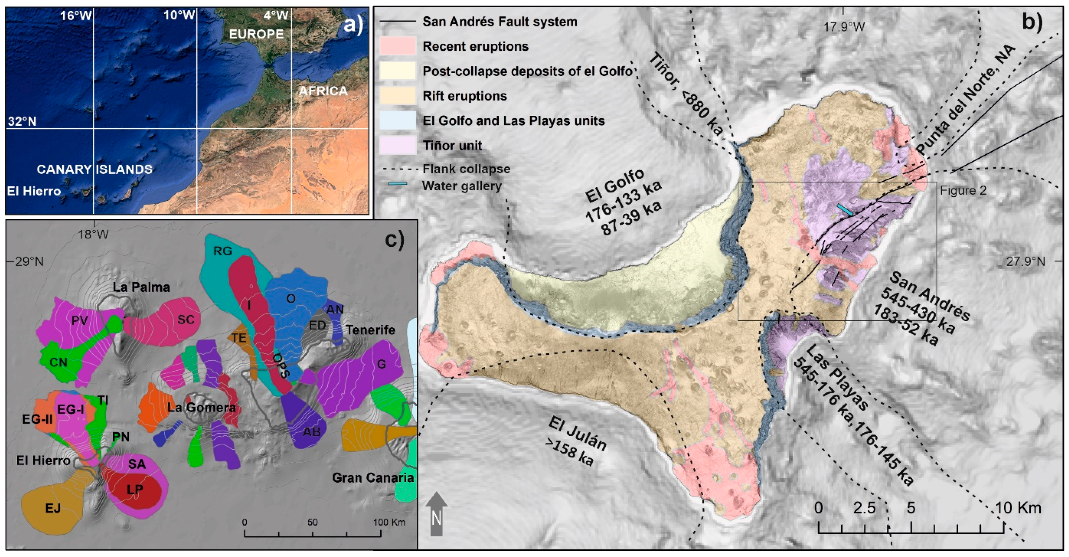
2. Study Area
2.1. Geological Settings
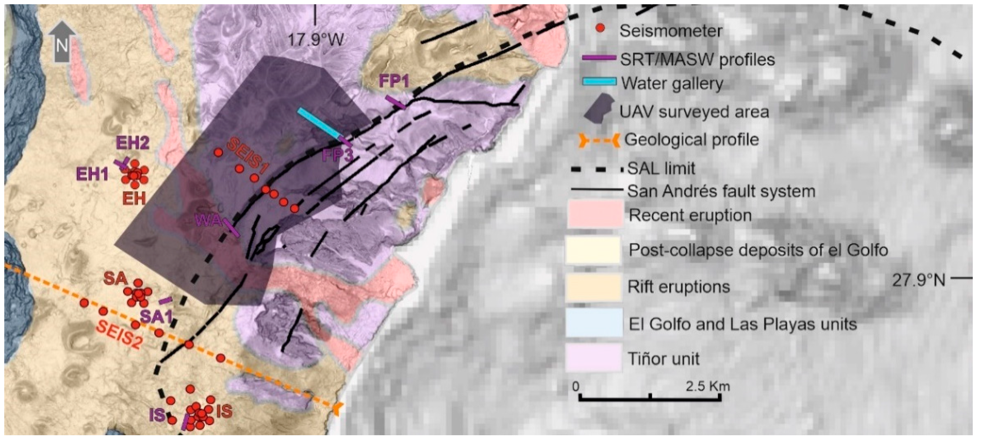
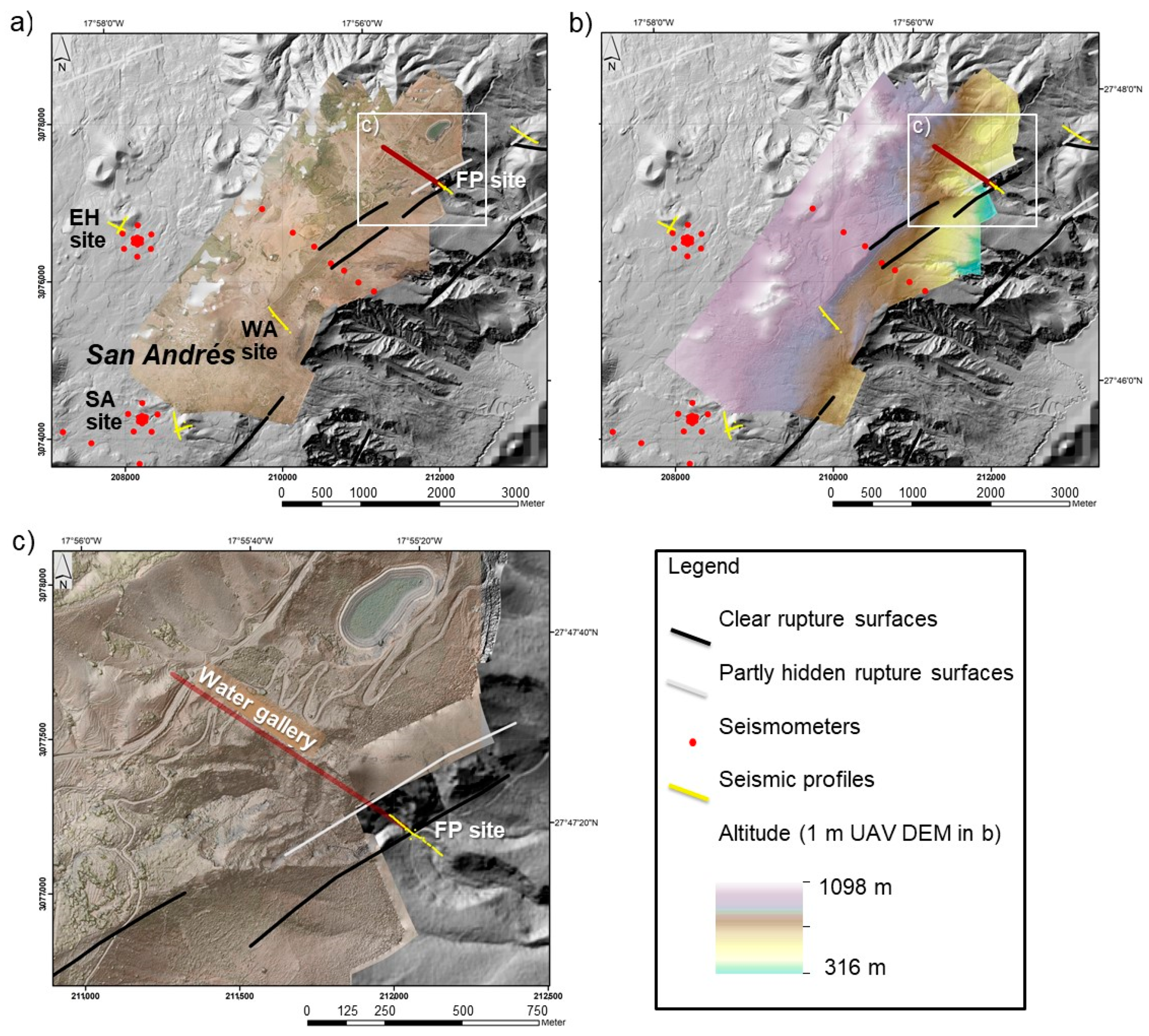
2.2. The San Andrés Landslide (SAL)
3. Methods
3.1. Passive Seismic Measurements
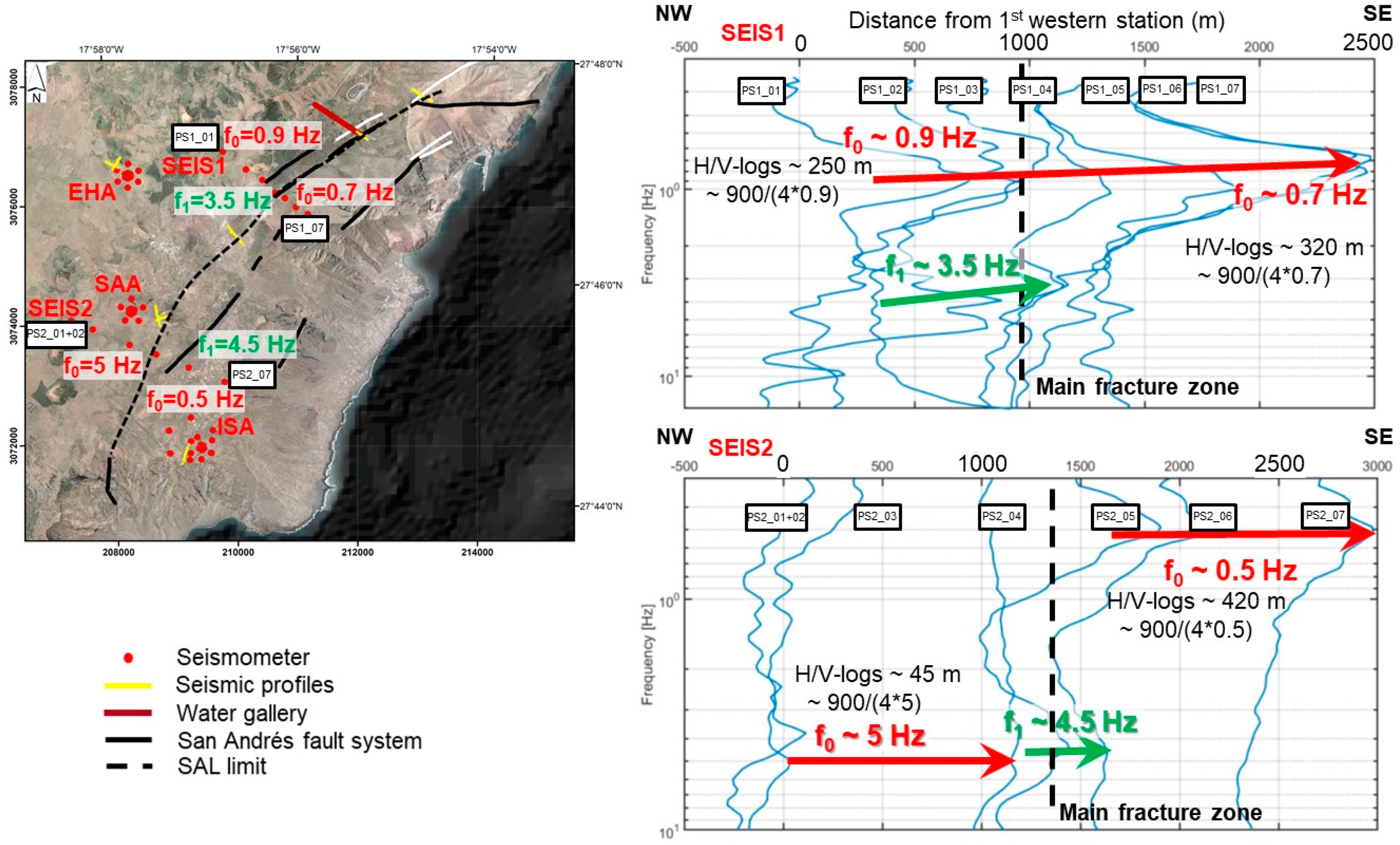
3.1.1. Horizontal-to-Vertical Spectral Ratio Technique (H/V)
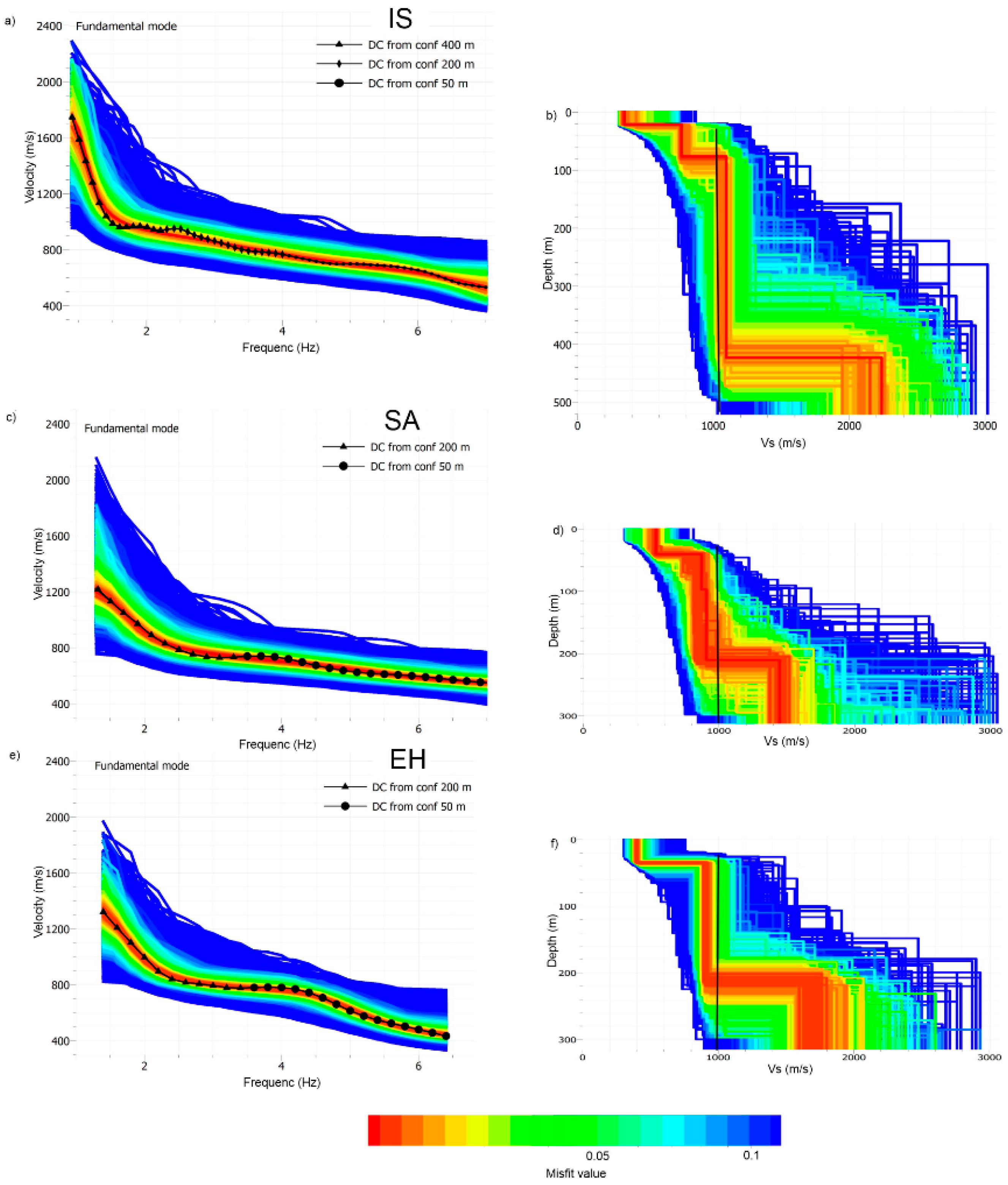
3.1.2. Ambient Noise Surface Wave Dispersion (Seismic Multichannel Array)
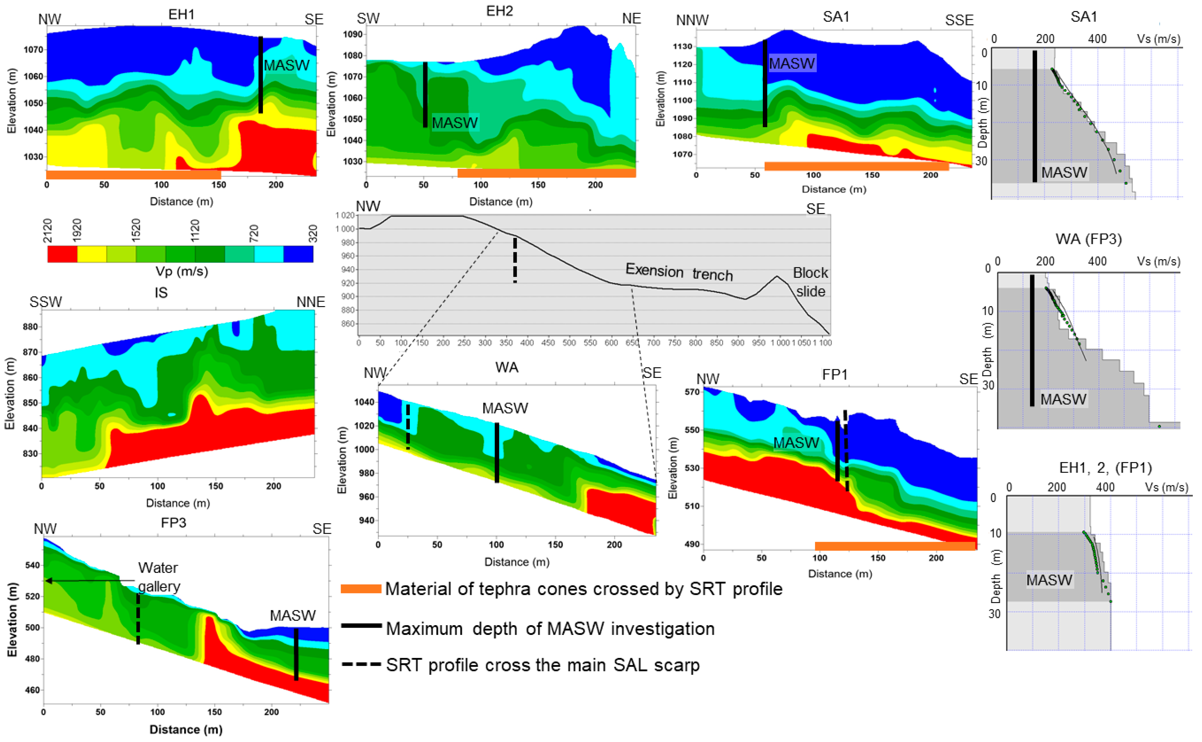
3.2. Active Seismic Measurements
3.3. UAV and DGPS Data Collection and Processing
3.4. Rocks Characterization
3.5. Results Visualization and Interpretation
4. Results
4.1. Results of the Geophysical Research
4.1.1. Active Seismic: SRT and MASW Results
4.1.2. Passive Seismic: Array and H/V Results
4.2. Laboratory and In-Situ Rock Properties Description
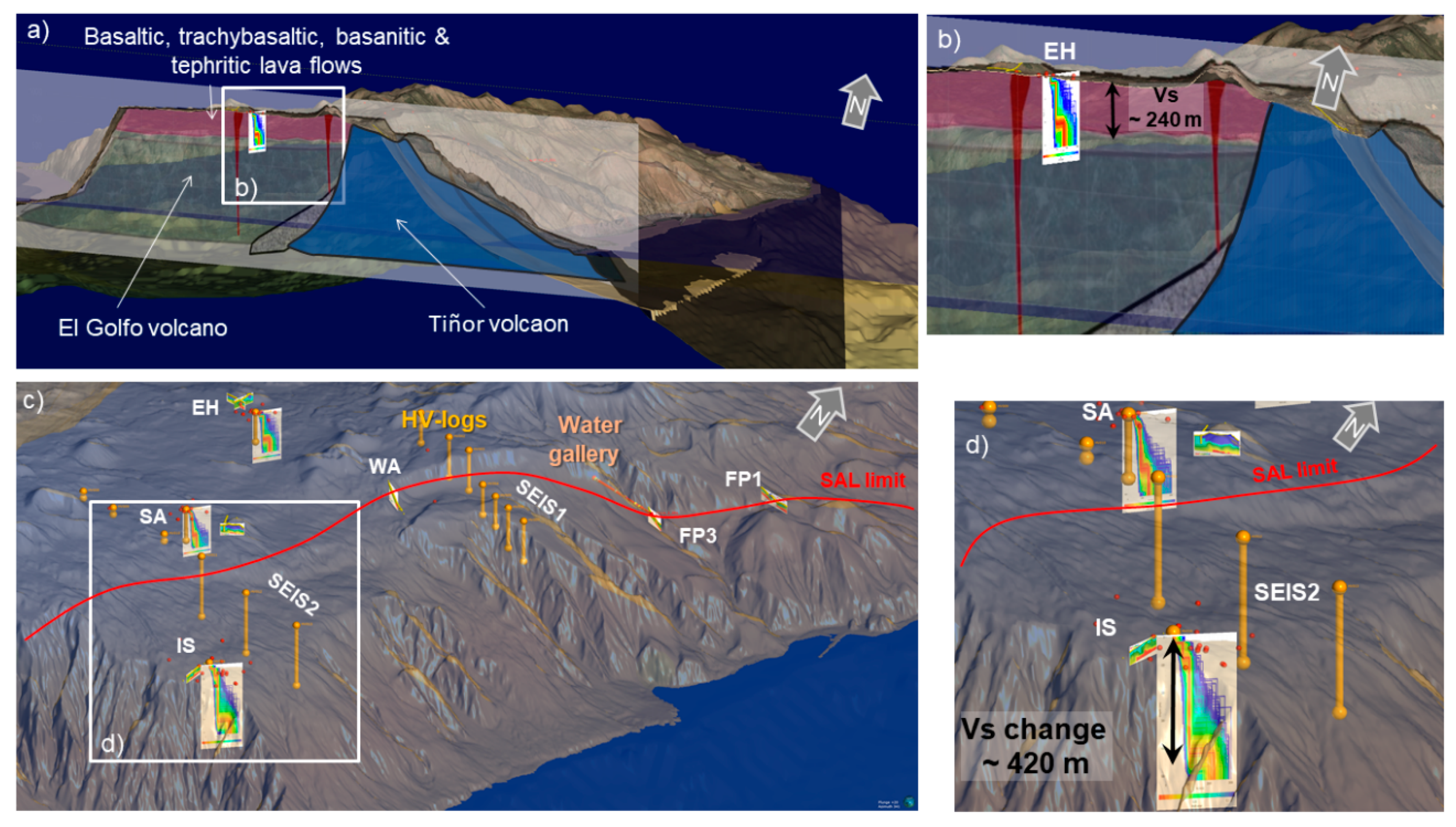
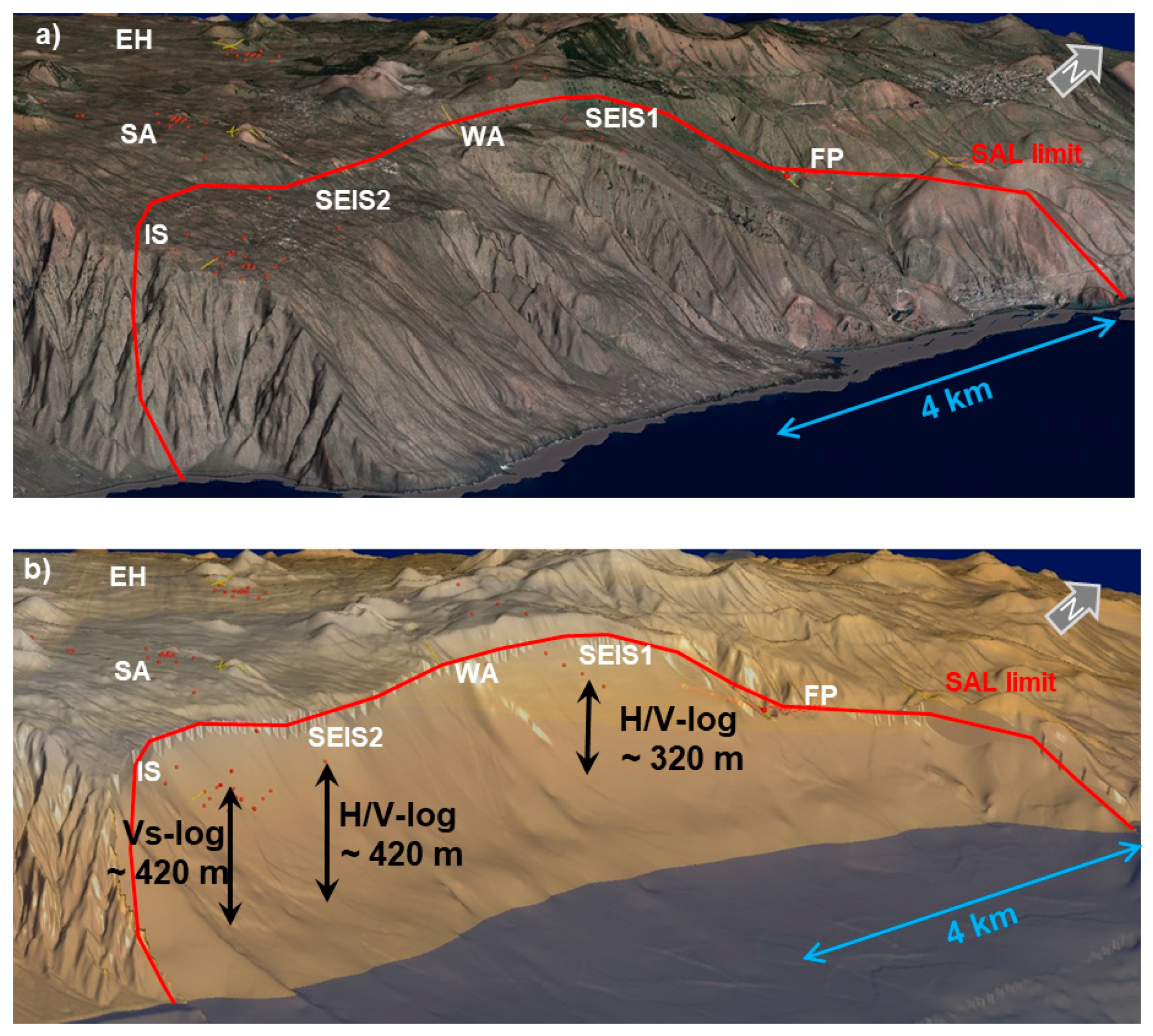
4.3. Geological Modeling
5. Discussion
6. Conclusions
Supplementary Materials
Author Contributions
Funding
Data Availability Statement
Acknowledgments
Conflicts of Interest
References
- Masson, D.G.; Le Bas, T.; Grevemeyer, I.; Weinrebe, W. Flank collapse and large-scale landsliding in the Cape Verde Islands, off West African. Geochem. Geophys. Geosyst. 2008, 9, Q07015. [Google Scholar] [CrossRef]
- Blahůt, J.; Balek, J.; Klimeš, J.; Rowberry, M.; Kusák, M.; Kalina, J. A comprehensive global database of giant landslides on volcanic islands. Landslides 2019, 16, 2045–2052. [Google Scholar] [CrossRef]
- Hunt, J.E.; Wynn, R.B.; Talling, P.J.; Masson, D.G. Multistage collapse of eight western Canary Island landslides in the last 1.5 Ma: Sedimentological and geochemical evidence from subunits in submarine flow deposits. Geochem. Geophys. Geosyst. 2013, 14, 2159–2181. [Google Scholar] [CrossRef] [Green Version]
- Hunt, J.E.; Jarvis, I. Prodigious submarine landslides during the inception and early growth of volcanic islands. Nat. Commun. 2017, 8, 2061. [Google Scholar] [CrossRef] [Green Version]
- León, R.; Somoza, L.; Urgeles, R.; Medialdea, T.; Ferrer, M.; Biain, A.; García-Crespo, J.; Mediato, J.; Galindo, I.; Yepes, J.; et al. Multi-event oceanic island landslides: New onshore-offshore insights from El Hierro Island, Canary Archipelago. Mar. Geol. 2017, 393, 156–175. [Google Scholar] [CrossRef]
- Blahůt, J.; Mitrovic-Woodell, I.; Baroň, I.; René, M.; Rowberry, M.; Blard, P.-H.; Hartvich, F.; Balek, J.; Meletlidis, S. Volcanic edifice slip events recorded on the fault plane of the San Andrés Landslide, El Hierro, Canary Islands. Tectonophysics 2020, 776, 228317. [Google Scholar] [CrossRef]
- Bernard, B.; Takarada, S.; Andrade, S.D.; Dufresne, A. Terminology and Strategy to Describe Large Volcanic Landslides and Debris Avalanches. In Volcanic Debris Avalanches: From Collapse to Hazard; Roverato, M., Dufresne, A., Procter, J., Eds.; Springer: Cham, Switzerland, 2021; pp. 51–73. [Google Scholar] [CrossRef]
- Owen, S.E.; Bürgmann, R. An increment of volcano collapse: Kinematics of the 1975 Kalapana, Hawaii, earthquake. J. Volcanol. Geother. Res. 2006, 150, 163–185. [Google Scholar] [CrossRef]
- Blahůt, J.; Klimeš, J. Causes and triggers of mass-movements: Volcanic activity. In Treatise on Geomorphology; Elsevier: Amsterdam, The Netherlands, 2021. [Google Scholar] [CrossRef]
- Day, S.; Carracedo, J.-C.; Guillou, H. Age and geometry of an aborted rift flank collapse: The San Andres fault system, El Hierro, Canary Islands. Geol. Mag. 1997, 134, 523–537. [Google Scholar] [CrossRef]
- Jongmans, D.; Garambois, S. Geophysical investigation of landslides: A review. Bullet. Société Géologique Fr. 2007, 178, 101–112. [Google Scholar] [CrossRef] [Green Version]
- Panzera, F.; Lombardo, G.; Monaco, C. New evidence of wavefield polarization on fault zone in the lower NE slope of Mt. Etna. It. J. Geosci. 2016, 135, 250–260. [Google Scholar] [CrossRef]
- Hussain, Y.; Schlögel, R.; Innocenti, A.; Hamza, O.; Iannucci, R.; Martino, S.; Havenith, H.-B. Review on the Geophysical and UAV-Based Methods Applied to Landslides. Remote Sens. 2022, 14, 4564. [Google Scholar] [CrossRef]
- Carracedo, J.-C.; Rodríguez Badiola, E.; Guillou, H.; De la Nuez, H.; Pérez Torrado, F. Geology and volcanology of the western Canaries: La Palma and El Hierro. Estud. Geológ. 2001, 57, 171–295. [Google Scholar]
- Delgado, J.; Galiana-Merino, J.J.; García-Tortosa, F.J.; Garrido, J.; Lenti, L.; Martino, S.; Soler-Earle, P.S.; Shearer, P.M. Characterization of global seismograms using an automatic-picking algorithm. Bull. Seism. Soc. Am. 1994, 84, 366–376. [Google Scholar]
- Ryberg, T.; Kirsch, M.; Haberland, C.; Tolosana-Delgado, R.; Viezzoli, A.; Gloaguen, R. Ambient seismic noise analysis of LARGE-N data for mineral exploration in the Central Erzgebirge, Germany. Solid Earth 2022, 13, 519–533. [Google Scholar] [CrossRef]
- Jornet-Monteverde, J.A.; Galiana-Merino, J.J.; Soler-Llorens, J.L. Design and implementation of a wireless recorder system for seismic noise array measurements. Sensors 2022, 22, 8103. [Google Scholar] [CrossRef] [PubMed]
- Hussain, Y.; Cardenas-Soto, M.; Martino, S.; Moreira, C.; Borges, W.; Hamza, O.; Martinez-Carvajal, H. Multiple geophysical techniques for investigation and monitoring of Sobradinho landslide, Brazil. Sustainability 2019, 11, 6672. [Google Scholar] [CrossRef] [Green Version]
- Mreyen, A.-S.; Cauchie, L.; Micu, M.; Onaca, A.; Havenith, H.-B. Multiple geophysical investigation to characterize massive slope failure deposits: Application to the Balta rockslide, Carpathians. Geoph. J. Int. 2021, 225, 1032–1047. [Google Scholar] [CrossRef]
- Calamita, G.; Serlenga, V.; Stabile, T.A.; Gallipoli, M.R.; Bellanova, J.; Bonano, M.; Perrone, A. An integrated geophysical approach for urban underground characterization: The Avigliano town (southern Italy) case study. Geomat. Nat. Haz. Risk 2019, 10, 412–432. [Google Scholar] [CrossRef] [Green Version]
- Chatzis, N.; Papazachos, C.; Theodoulidis, N.; Hatzidimitriou, P.; Vougioukalakis, G.; Paulatto, M.; Heath, B.; Hooft, E.; Toomey, D.; Anthymidis, M.; et al. Metamorphic bedrock geometry of Santorini using HVSR information and geophysical modeling of ambient noise and active-source surface-wave data. J. Volcan. Geotherm. Res. 2022, 432, 107692. [Google Scholar] [CrossRef]
- Natali, M.; Lidal, E.M.; Parulek, J.; Viola, I.; Patel, D. Modeling terrains and subsurface geology. In Eurographics 2013—State of the Art Reports; The Eurographics Association: Eindhoven, The Netherlands, 2013; pp. 155–173. [Google Scholar] [CrossRef]
- Caumon, G.; Collon-Drouaillet, P.; De Veslud, C.L.C.; Viseur, S.; Sausse, J. Surface based 3D modeling of geological structures. Math. Geosci. 2009, 41, 927–945. [Google Scholar] [CrossRef] [Green Version]
- Lerch, C.; Hoppe, A. Development of a geological 3D-model for improved calculations of groundwater vulnerability. Grundwasser 2007, 12, 144–153. [Google Scholar] [CrossRef]
- Havenith, H.-B.; Torgoev, I.; Ischuk, A. Integrated Geophysical-Geological 3D Model of the Right-Bank Slope Downstream from the Rogun Dam Construction Site, Tajikistan. Int. J. Geophys. 2018, 2018, 1641789. [Google Scholar] [CrossRef] [Green Version]
- Mreyen, A.S.; Donati, D.; Elmo, D.; Donze, F.V.; Havenith, H.-B. Dynamic numerical modelling of co-seismic landslides using the 3D distinct element method: Insights from the Balta rockslide (Romania). Eng. Geol. 2022, 307, 106774. [Google Scholar] [CrossRef]
- Lipman, P.W.; Lockwood, J.P.; Okamura, R.T.; Swanson, D.A.; Yamashita, K.M. Ground deformation associated with the 1975 Magnitude-7.2 earthquake and resulting changes in activity of Kilauea volcano, Hawaii. In The USGS Professional Paper 1276; Gyan Books Pvt. Ltd.: Delhi, India, 1985; p. 45. [Google Scholar] [CrossRef] [Green Version]
- Hildenbrand, A.; Marques, F.; Catalao, J.; Catita, C.; Costa, A. Large scale active slump of the southeastern flank of Pico Island, Azores. Geology 2012, 40, 939–942. [Google Scholar] [CrossRef]
- Blahůt, J.; Baroň, I.; Sokol, L.; Meletlidis, S.; Klimeš, J.; Rowberry, M.; Melichar, R.; García-Cañada, L.; Martí, X. Large landslide stress states calculated during extreme climatic and tectonic events on El Hierro, Canary Islands. Landslides 2018, 15, 1801–1814. [Google Scholar] [CrossRef]
- Blahůt, J.; Olejár, F.; Rott, J.; Petružálek, M. Current stability modelling of an incipient San Andrés giant landslide on El Hierro, Canaries, Spain—First attempt using limited input data. Acta Geodyn. Geomat. 2020, 17, 89–99. [Google Scholar] [CrossRef]
- Blahůt, J.; Balek, J.; Eliaš, M.; Meletlidis, S. 3D Dilatometer time-series analysis for a better understanding of the dynamics of a giant slow-moving landslide. App. Sci. 2020, 10, 5469. [Google Scholar] [CrossRef]
- Schmincke, H.-U.; Sumita, M. Geological Evolution of the Canary Islands; Görres Druckerei und Verlag: Koblenz, Germany, 2010. [Google Scholar]
- Becerril, L.; Galindo, I.; Martí, J.; Gudmundsson, A. Three-armed rifts or masked radial pattern of eruptive fissures? The intriguing case of El Hierro volcano (Canary Islands). Tectonophysics 2015, 647, 33–47. [Google Scholar] [CrossRef]
- Guillou, H.; Carracedo, J.C.; Pérez Torrado, F.; Rodríguez Badiola, E. K-Ar ages and magnetic stratigraphy of a hotspot-induced, fast grown oceanic island: El Hierro, Canary Islands. J. Volc. Geotherm. Res. 1996, 73, 141–155. [Google Scholar] [CrossRef]
- Becerril, L.; Ubide, T.; Sudo, M.; Martí, J.; Galindo, I.; Galé, C.; Morales, J.; Yepes, J.; Lago, M. Geochronological constraints on the evolution of El Hierro (Canary Islands). J. Afr. Earth Sci. 2016, 113, 88–94. [Google Scholar] [CrossRef]
- Risica, G.; Di Roberto, A.; Speranza, F.; Del Carlo, P.; Pompilio, M.; Meletlidis, S.; Todrani, A. Reconstruction of the subaerial Holocene volcanic activity through paleomagnetic and 14C dating methods: El Hierro (Canary Islands). J. Volcan. Geotherm. Res. 2022, 425, 107526. [Google Scholar] [CrossRef]
- Stroncik, N.; Klügel, A.; Hansteen, T. The magmatic plumbing system beneath El Hierro (Canary Islands): Constraints from phenocrysts and naturally quenched basaltic glasses in submarine rocks. Contrib. Miner. Petrol. 2009, 157, 593. [Google Scholar] [CrossRef]
- López, C.; Blanco, M.J.; Abella, R.; Brenes, B.; Cabrera Rodríguez, V.; Casas, B.; Domínguez Cerdeña, I.; Felpeto, A.; Fernández De Villalta, M.; Del Fresno, C.; et al. Monitoring the volcanic unrest of El Hierro (Canary Islands) before the onset of the 2011–2012 submarine eruption. Geophys. Res. Lett. 2012, 39, L13303. [Google Scholar] [CrossRef]
- Benito-Saz, M.; Parks, M.; Sigmundsson, F.; Hooper, A.; García-Cañada, L. Repeated magmatic intrusions at El Hierro Island following the 2011–2012 submarine eruption. J. Volcanol. Geotherm. Res. 2017, 344, 79–91. [Google Scholar] [CrossRef] [Green Version]
- Meletlidis, S.; Di Roberto, A.; Domínguez Cerdeña, I.; Pompilio, M.; García-Cañada, L.; Bertagnini, A.; Benito-Saz, M.; Del Carlo, P.; Sainz-Maza Aparicio, S. New insight into the 2011–2012 unrest and eruption of El Hierro Island (Canary Islands) based on integrated geophysical, geodetical, and petrological data. Ann. Geophys. 2015, 58, S0546. [Google Scholar] [CrossRef]
- Masson, D. Catastrophic collapse of the volcanic island of Hierro 15 ka ago and the history of landslides in the Canary Islands. Geology 1996, 24, 231–234. [Google Scholar] [CrossRef]
- Urgeles, R.; Canals, M.; Baraza, J.; Alonso, B. The submarine El Golfo debris avalanche and the Canary debris flow, west Hierro Island: The last major slides in the Canary Archipelago. Geogaceta 1996, 20, 390–393. [Google Scholar]
- Urgeles, R.; Canals, M.; Baraza, J.; Alonso, B.; Masson, D. The most recent megalandslides on the Canary Islands: The El Golfo debris avalanche and the Canary debris flow, west El Hierro Island. J. Geophys. Res. Solid Earth 1997, 102, 20305–20323. [Google Scholar] [CrossRef]
- Carracedo, J.-C.; Day, S.; Guillou, H.; Pérez Torrado, F. Giant quaternary landslides in the evolution of La Palma and El Hierro, Canary Islands. J. Volcanol. Geotherm. Res. 1999, 94, 169–190. [Google Scholar] [CrossRef]
- Masson, D.; Watts, A.; Gee, M.; Urgeles, R.; Mitchell, N.; Le Bas, T.; Canals, M. Slope failures on the flanks of the western Canary Islands. Earth Sci. Rev. 2002, 57, 1–35. [Google Scholar] [CrossRef]
- Longpré, M.; Chadwick, J.; Wijbrans, J.; Iping, R. Age of the El Golfo debris avalanche, El Hierro (Canary Islands): New constraints from laser and furnace 40Ar/39Ar dating. J. Volcanol. Geotherm. Res. 2011, 203, 76–80. [Google Scholar] [CrossRef]
- Becerril, L.; Galve, J.; Morales, J.; Romero, C.; Sánchez, N.; Martí, J.; Galindo, I. Volcanostructure of El Hierro (Canary Islands). J. Maps 2016, 12 (Suppl. 1), 43–52. [Google Scholar] [CrossRef] [Green Version]
- Carracedo, J.-C.; Troll, V. The Geology of Canary Islands; Elsevier: Amsterdam, The Netherlands, 2016. [Google Scholar]
- Blahůt, J.; Klimeš, J.; Rowberry, M.; Kusák, M. Database of giant landslides on volcanic islands—First results from the Atlantic Ocean. Landslides 2018, 15, 823–827. [Google Scholar] [CrossRef]
- Moscardelli, L.; Wood, L. New classification system for mass transport complexes in offshore Trinidad. Basin Res. 2008, 20, 73–98. [Google Scholar] [CrossRef]
- Klimeš, J.; Yepes, J.; Becerril, L.; Kusák, M.; Galindo, I.; Blahůt, J. Development and recent activity of the San Andrés landslide on El Hierro, Canary Islands, Spain. Geomorphology 2016, 261, 119–131. [Google Scholar] [CrossRef] [Green Version]
- Duffield, W. Structure and Origin of the Koae Fault System, Kilauea Volcano, Hawaii; Professional Paper 856; U.S. Government Publishing Office: Washington, DC, USA, 1975; p. 12.
- Krastel, S.; Schmincke, H.-U.; Jacobs, C.L.; Rihm, R.; Le Bas, T.P.; Alibés, B. Submarine landslides around the Canary Islands. J. Geophys. Res. Solid Earth 2001, 106, 3977–3997. [Google Scholar] [CrossRef]
- Gómez Sainz de Aja, J.; Klein, E.; Ruiz García, M.; Balcells Herrera, R.; Del Pozo, M.; Galindo, E.; La Moneda, E. Mapa Geológico de España, Escala 1:25 000, Valverde (Isla de El Hierro), Hoja N° 1105-II, Memoria; Instituto Geológico y Minero de España: Madrid, Spain, 2010; p. 96. [Google Scholar]
- Troll, V.; Carracedo, J.C. (Eds.) The Geology of El Hierro. In The Geology of Canary Islands; Elsevier: Amsterdam, The Netherlands, 2016; pp. 43–99. [Google Scholar]
- Blahůt, J.; Klimeš, J.; Meletlidis, S.; Balek, J.; Rowberry, M.; Baroň, I. A decade of monitoring and research on the San Andrés megalandslide on El Hierro, Canary Islands, Spain. In Advances in Natural Hazards and Volcanic Risks: Shaping a Sustainable Future—Proceedings of the 3rd International Workshop on Natural Hazards (NATHAZ22), Terceira Island—Azores 2022; Springer ASTI Series; Springer: Berlin/Heidelberg, Germany, 2022. [Google Scholar]
- MDT05 Modelo Digital del Terreno de España. Sheet PNOA-MDT05-REGCAN95-HU28-1105-1108-LID.ASC. 2015. Available online: https://centrodedescargas.cnig.es/CentroDescargas (accessed on 13 March 2018).
- Insituto Hidrográfico de la Marina, Cuartel General de la Armada, Spain. IHM Bathymetric Data of the Canary Islands. 2016. Available online: http://portal.emodnet-bathymetry.eu (accessed on 1 January 2018).
- Nakamura, Y. A method for dynamic characteristics estimation of subsurface using microtremor on the ground surface. Railw. Tech. Res. Inst. Quart. Rep. 1989, 30, 25–33. [Google Scholar]
- Ibs-von Seht, M.; Wohlenberg, J. Microtremor measurements used to map thickness of soft sediments. Bull. Seism. Soc. Am. 1999, 89, 250–259. [Google Scholar] [CrossRef]
- Capon, J. High-resolution frequency-wavenumber spectrum analysis. Proc. IEEE 1969, 57, 1408–1418. [Google Scholar] [CrossRef] [Green Version]
- Rost, S.; Thomas, C. Array seismology: Methods and applications. Rev. Geophys. 2002, 40, 1–2. [Google Scholar] [CrossRef] [Green Version]
- Wathelet, M.; Chatelain, J.L.; Cornou, C.; Giulio, G.D.; Guillier, B.; Ohrnberger, M.; Savvaidis, A. Geopsy: A user-friendly open-source tool set for ambient vibration processing. Seismol. Res. Lett. 2020, 91, 1878–1889. [Google Scholar] [CrossRef]
- Shen, C.; Xu, Y.; Pan, Y.; Wang, A.; Gao, L. Sensitivities of phase-velocity dispersion curves of surface waves due to high-velocity-layer and low-velocity-layer models. J. Appl. Geophys. 2016, 135, 367–374. [Google Scholar] [CrossRef]
- Guedes, V.J.C.B.; Borges, W.R.; Da Cunha, L.S.; Maciel, S.T.R. Characterization of an earth dam in Brazil from seismic refraction tomography and multichannel analysis of surface waves. J. Appl. Geophys. 2023, 208, 104893. [Google Scholar] [CrossRef]
- Hayashi, K. Data Acquisition and Analysis of Active and Passive Surface Waves. In Symposium on the Application of Geophysics to Environmental and Engineering Problems Short Course Notes; Environmental and Engineering Geophysical Society: Denver, CO, USA, 2003; p. 106. [Google Scholar]
- Marinos, P.; Hoek, E. GSI: A geologically friendly tool for rock mass strength estimation. In Proceedings of the GeoEng2000 at the International Conference on Geotechnical and Geological Engineering, Lancaster, PA, USA, 19–24 November 2000; Technomic Publishers: Lancaster, PA, USA, 2000. [Google Scholar]
- Becerril, L. Volcano-Structural Study and Long-Term Volcanic Hazard Assessment on El Hierro Island (Canary Islands). Ph.D. Thesis, University of Zaragoza, Zaragoza, Spain, 2014. ISBN 978-84-617-3444-3. [Google Scholar]
- ISRM. The Complete ISRM Suggested Methods for Rock Characterization, Testing and Monitoring: 1974–2006; Ulusay, R., Hudson, J.A., Eds.; ISRM: Ankara, Turkey, 2007. [Google Scholar]
- Cai, M.; Kaiser, P.K.; Tasaka, Y.; Minami, M. Determination of residual strength parameters of jointed rock masses using the GSI system. Int. J. Rock Mech. Min. Sci. 2007, 44, 247–265. [Google Scholar] [CrossRef]
- Hoek, E.; Carranza-Torres, C.; Corkum, B. Hoek-Brown Failure Criterion—2002 Edition. In Proceedings of the NARMS-Tac, Toronto, ON, Canada, 4–6 November 2002; Volume 1, pp. 267–273. [Google Scholar]
- Sapia, V.; Oldenborger, G.A.; Jørgensen, F.; Pugin, A.J.-M.; Marchetti, M.; Viezzoli, A. 3D modeling of buried valley geology using airborne electromagnetic data. Interpretation 2015, 3, SAC9–SAC22. [Google Scholar] [CrossRef]
- Davarpanah, S.M.; Ván, P.; Vásárhelyi, B. Investigation of the relationship between dynamic and static deformation moduli of rocks. Geomech. Geophys. Geo-Energy Geo-Resour. 2020, 6, 29. [Google Scholar] [CrossRef] [Green Version]
- Al-Harthi, A.A.; Al-Amri, R.M.; Shehata, W.M. The porosity and engineering properties of vesicular basalt in Saudi Arabia. Eng. Geol. 1999, 54, 313–320. [Google Scholar] [CrossRef]
- Read, S.A.L.; Richards, L.R. Guidelines for use of tensile data in the calculation of the Hoek-Brown constant mi. In Proceedings of the ISRM Congress, Montreal, QC, Canada, 10–14 May 2015; pp. 10–13. [Google Scholar]
- Hoek, E. Practical Rock Engineering; Rocscience: Toronto, ON, Canada, 2007; p. 342. [Google Scholar]
- Marions, P.G.; Marinos, V.; Hoek, E. The Geological Strength Index (GSI): A characterization tool for assessing engineering properties of rock masses. In Proceedings of the International Workshop on Rock Mass Classification in Underground Mining, Vancover, BC, Canada, 13–18 July 2007. [Google Scholar] [CrossRef]
- Chalupa, V.; Pánek, T.; Tábořík, P.; Klimeš, J.; Hartvich, F.; Grygar, R. Deep-seated gravitational slope deformations controlled by the structure of flysch nappe outlier: Insights from large scale electrical resistivity tomography survey and LiDAR mapping. Geomorphology 2018, 321, 174–187. [Google Scholar] [CrossRef]
- Tang, C.L.; Hu, J.C.; Lin, M.L.; Angelier, J.; Lu, C.Y.; Chan, Y.C.; Chu, H.T. The Tsaoling landslide triggered by the Chi-Chi earthquake, Taiwan: Insights from a discrete element simulation. Eng. Geol. 2009, 106, 1–19. [Google Scholar] [CrossRef]
- Lemaire, E.; Mreyen, A.-S.; Dufresne, A.; Havenith, H.-B. Analysis of the influence of structural geology on the massive seismic slope failure potential supported by numerical modelling. Geosciences 2020, 10, 323. [Google Scholar] [CrossRef]


| Rock Constituent | Compact Basalt | Porous Basalt | ||||
|---|---|---|---|---|---|---|
| Content [%] | Grain size [mm] | Description | Content [%] | Grain Size [mm] | Description | |
| Groundmass (plagiocalse, pyroxene) | 80–90% | <0.1 | No preferential orientation, alteration, microcracks | 30–50% | <0.3 | No preferential orientation, alteration, microcracks |
| Olivine fenocrysts | 5–10% | 0.5–1 | No preferential orientation, and alteration, low microcrack density | 20–30% | 1–1.5 | No preferential orientation, medium alteration, high microcrack density |
| Volcanic glass | 0% | - | - | 10–20% | 0.3–1.5 | No preferential orientation, alteration, microcracks |
| Macropores | <1% | 0.1–0.3 | Ellipsoidal shape without preferential orientation | 2–5% | 0.2–1 | Ellipsoidal shape without preferential orientation |
| Rocks | ρd_AV | ρs | n | VP | VS | |
|---|---|---|---|---|---|---|
| [g/cm3] | [g/cm3] | [%] | [m/s] | [m/s] | ||
| Compact basalt | mean | 2.931 | 2.942 | 0.367 | 5768 | 3347 |
| N | 5 | 3 | 5 | 5 | 5 | |
| std | 0.004 | 0.003 | 0.144 | 0.083 | 0.065 | |
| Porous basalt | mean | 2.836 | 2.929 | 3.176 | 4647 | 2836 |
| N | 3 | 3 | 3 | 3 | 3 | |
| std | 0.034 | 0.005 | 1.175 | 0.070 | 0.034 |
| Rocks | Elastic Moduli | E | v | u | K |
|---|---|---|---|---|---|
| [GPa] | [GPa] | [GPa] | |||
| Porous basalt | DYNAMIC | 46.0 | 0.20 | 19.1 | 25.8 |
| STATIC | 36.4 | 0.21 | 15.0 | 21.0 | |
| Compact basalt | DYNAMIC | 81.9 | 0.25 | 32.9 | 53.8 |
| STATIC | 59.8 | 0.25 | 24.0 | 39.7 |
| Rocks | Principle Stress | BTS | DTS | UCS | TCS | ||
|---|---|---|---|---|---|---|---|
| [MPa] | [MPa] | [MPa] | [MPa] | ||||
| Porous basalt | σ1 | −10.2 | −9.2 | 0.0 | 7.0 | 15.0 | 25.0 |
| σ1 | - | 0.0 | 86.5 | 150.7 | 179.5 | 207.9 | |
| Compact basalt | σ3 | −11.4 | −10.3 | 0.0 | 7.0 | 15.0 | 30.0 |
| σ1 | - | 0.0 | 343.9 | 411.5 | 441.1 | 554.6 | |
| Rock Type | Rock State | GSI | s | m | a | UCS | DTS |
|---|---|---|---|---|---|---|---|
| [-] | [-] | [-] | [-] | [MPa] | [MPa] | ||
| Basalt Porous | Intact | 100.0 | 1.000 | 10.636 | 0.500 | 98.700 | 9.20 |
| Rock mass | 80.0 | 0.108 | 5.207 | 0.501 | 32.436 | 2.90 | |
| Residual | 40.0 | 0.001 | 1.300 | 0.511 | 3.121 | 0.45 | |
| Basalt Compact | Intact | 100.0 | 1.000 | 27.574 | 0.500 | 284.600 | 10.00 |
| Rock mass | 80.0 | 0.108 | 13.499 | 0.501 | 93.529 | 2.30 | |
| Residual | 40.0 | 0.001 | 3.235 | 0.511 | 9.000 | 0.24 |
Disclaimer/Publisher’s Note: The statements, opinions and data contained in all publications are solely those of the individual author(s) and contributor(s) and not of MDPI and/or the editor(s). MDPI and/or the editor(s) disclaim responsibility for any injury to people or property resulting from any ideas, methods, instructions or products referred to in the content. |
© 2023 by the authors. Licensee MDPI, Basel, Switzerland. This article is an open access article distributed under the terms and conditions of the Creative Commons Attribution (CC BY) license (https://creativecommons.org/licenses/by/4.0/).
Share and Cite
Klimeš, J.; Hussain, Y.; Mreyen, A.-S.; Cauchie, L.; Schlögel, R.; Piroton, V.; Petružálek, M.; Blahůt, J.; René, M.; Meletlidis, S.; et al. New Insights into the Internal Structures and Geotechnical Rock Properties of the Giant San Andrés Landslide, El Hierro Island, Spain. Remote Sens. 2023, 15, 1627. https://doi.org/10.3390/rs15061627
Klimeš J, Hussain Y, Mreyen A-S, Cauchie L, Schlögel R, Piroton V, Petružálek M, Blahůt J, René M, Meletlidis S, et al. New Insights into the Internal Structures and Geotechnical Rock Properties of the Giant San Andrés Landslide, El Hierro Island, Spain. Remote Sensing. 2023; 15(6):1627. https://doi.org/10.3390/rs15061627
Chicago/Turabian StyleKlimeš, Jan, Yawar Hussain, Anne-Sophie Mreyen, Léna Cauchie, Romy Schlögel, Valentine Piroton, Matěj Petružálek, Jan Blahůt, Miloš René, Stavros Meletlidis, and et al. 2023. "New Insights into the Internal Structures and Geotechnical Rock Properties of the Giant San Andrés Landslide, El Hierro Island, Spain" Remote Sensing 15, no. 6: 1627. https://doi.org/10.3390/rs15061627