Absolute Localization of Targets Using a Phase-Measuring Sidescan Sonar in Very Shallow Waters

Abstract

The detection, classification, and localization of targets or features on the seafloor in acoustic data are critical to many disciplines. This is most important in cases where human safety is in jeopardy, such as hazards to navigation, mitigation of mine countermeasures, or unexploded ordnance. This study quantifies the absolute localization of targets, in the form of inert unexploded ordnance, in very shallow waters (2–3 m) on two intertidal bottom types in a meso-tidal environment (tide range = ~3.0 m). The two sites, a sandy intertidal flat and a mixed sand and gravel beach with abundant cobble-sized material, were seeded at low tide with targets (wax-filled 60-, 81-, 105- and 155-mm, projectile and mortar shells). An RTK-GPS was used to collect positional data for the targets and an unoccupied aerial system (UAS) survey was conducted on both sites. At the next high-tide, a vessel-based acoustic survey was performed, and at the subsequent low tide, the targets were re-surveyed with RTK-GPS. We focus here on the sidescan backscatter from a phase-measuring sidescan sonar (PMSS) and the sources of uncertainty for absolute localization. A total of 1426 calls of acoustic targets were made within the sidescan backscatter data, yielding an accuracy of 0.41 ± 0.26 m, with 98.9% of all calls <1 m from their absolute location. Distance from nadir was the most significant source of uncertainty, and targets between 3–7 m had the lowest uncertainty (0.32 ± 0.23 m) with increasing values toward and away from nadir. Bathymetry and bathymetry-mode backscatter were less useful for the detection and classification of targets compared to sidescan backscatter, but once detected, the accuracy of absolute localization were similar. This is likely due to target calls from these two datasets that were orders of magnitude less and that focused on the larger sized targets, thus more work is needed to better understand these differences. Lastly, the absolute localization of targets detected on sandy and cobble bottoms for all datasets were statistically similar. These acoustic instruments, their datasets, and methods presented herein can better document the absolute localization within acoustic data for many uses in very shallow waters.

1. Introduction

The localization of natural and anthropogenic features on the seafloor via acoustic instruments is important for many applications from change detection, spatial analysis, and habitat mapping to marine debris mitigation, underwater construction, and marine spatial planning [1,2,3,4,5,6]. The precise geographic localization of a target or feature is critical for applications in underwater environments where human safety is involved, such as mine countermeasures and work with unexploded ordnance (UXO). In fact, for remedial action, an absolute positioning accuracy of <1 m is needed and has not, as of yet, been established using standard acoustic sensors [7]. This is a major drawback for acoustic sensors and platforms as otherwise they are well-suited for detecting and classifying munitions due to their high frequency, high resolution datasets, large standoff distances from hazardous areas, and their ability to map large areas rapidly [7,8].

There are over 4.0 × 10⁶ ha (1.0 × 10⁷ ac) of UXO in the waters of the United States [9,10]. An ongoing project (MR19-B4-5079) funded by the Environmental Security Technology Certification Program (ESTCP) within the U.S. Department of Defense (DoD) Munitions Response Program responded to the call for improving the detection, classification, and localization of UXO in water depths from 0–5 m, making phase-measuring sidescan sonars (PMSS) suitable for these types of investigations. This paper, using a subsample of data collected for the DoD project, focuses on the localization of targets, proud of the seafloor, in 1.5–2.5 m of water on sand, as well as mixed sand and gravel intertidal zones.

Historically, the use of sidescan sonar has been the primary instrument for the detection, classification, and localization (DCL) of UXO and mine countermeasures [11]. For buried and/or partially buried UXO, the addition of sub-bottom profilers, magnetometers, and more recently, synthetic aperture sonars, have also been used [12,13,14,15]. While these instruments have proven useful for detection and classification, the absolute localization of the targets, while critical, has proven to be sub-optimal, particularly with regard to UXO remediation efforts. The detection and classification of UXO with these instruments are typically conducted with towed systems, and thus, estimates of the localization of the targets must begin with the positional uncertainty of the sensor [8]. The same challenges exist for autonomous underwater vessels (AUV) with regard to absolute localization [16,17].

PMSSs and studies using them have recently become more prevalent due to the utility of mapping in very shallow waters and the existing studies on storm-related processes [18,19], benthic habitat mapping [20,21,22,23,24,25], impacts of hydraulic clamming [26,27], and a myriad of other types of studies in the nearshore [28].

The use of multibeam echosounders (MBES), which must be mounted to the survey vessel in order to accurately create three-dimensional surfaces of the seafloor [29], have been used with regard to the DCL of UXO [30,31]. Consequently, there is an assumed increase in the absolute positional accuracy of targets in the data even though this is not discussed in these papers, further, there seems to be a lack of study in the peer-reviewed literature on the absolute positional accuracy of targets within acoustic data. There are very recent studies that discuss PMSSs with regard to survey platforms, data acquisition and processing [28,32,33], associated uncertainties [34], and in relation to MBES data [35].

This study seeks to quantify the absolute localization of targets in very shallow waters (~2 m) using a phase-measuring sidescan sonar (PMSS). These instruments provide similar data streams to multibeam echosounders, but the former has unique characteristics that substantially improve the effectiveness of survey work in very shallow waters. As part of a larger study to detect, classify, and localize unexploded ordnance, we utilize the high tidal range to seed intertidal areas with targets and collect positional data at low tide. Then, we collect vessel-based acoustic data at the next high tide and return to resurvey and retrieve targets at the subsequent low tide. The study sites also have variable bottom types that allow for the localization analysis to take bottom grain size (e.g., mud, sand, and gravel) into account.

While there are many studies that document the relative localization of targets or features in sidescan data, the authors have found a dearth of peer-reviewed literature related to absolute localization. Therefore, this paper is focused solely on quantifying the localization of targets with a priori knowledge of their presence/absence and geographic position. The primary dataset, the dual frequency sidescan sonar imagery, or sidescan backscatter, provides two-dimensional geographic position data. A subset of the acoustic data from the same instrument, the swath bathymetry and bathymetry-mode backscatter, (BMB) were also examined in order to document the relative and geographic positional accuracy of multiple data streams from a particular acoustic instrument. A full examination of these datasets warrants separate papers, one of which relating to BMB from a PMSS as can be seen in this volume [36], and another on swath bathymetry data from a PMSS which is in preparation [37]. It is believed that if the methods developed here are followed closely but adapted as needed to relevant conditions and instrument suites, the quantification of the geographic positional uncertainties of targets and/or features in acoustic data can be further developed and improved upon. Lastly, due to the intertidal location of the mapping efforts, UAS data are also discussed as they relate to the relative and absolute localization of the objects.

2. Materials and Methods

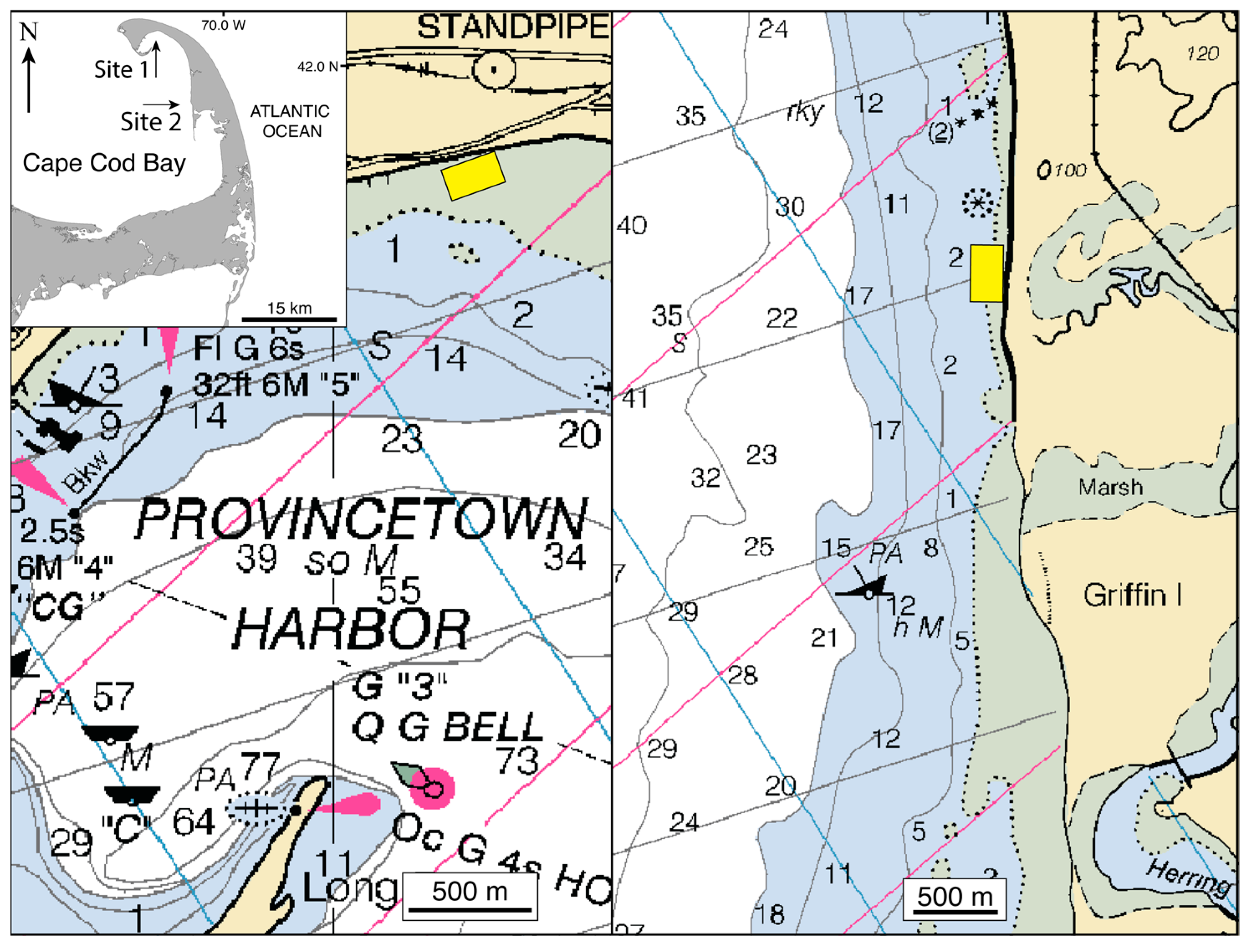
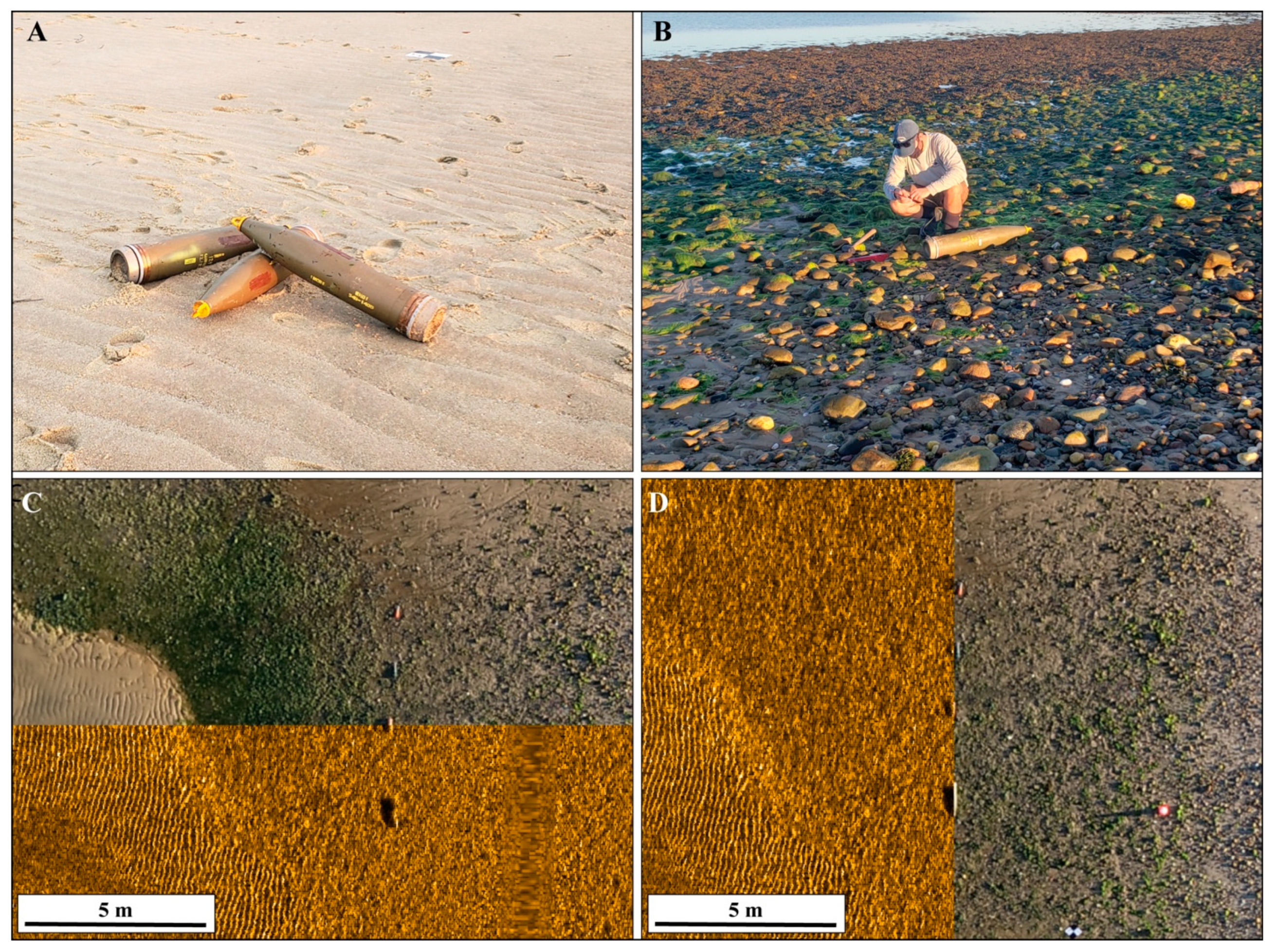
2.1. Field Setting

The material comprising Cape Cod, Massachusetts, USA was deposited during the last deglaciation, approximately 22 kya [38]. The glacial history of the region and subsequent reworking during the Holocene are responsible for the variability in seafloor habitats.

The data from the vessel-based acoustic surveys referred to in this study took place in Cape Cod Bay, a large mesotidal embayment in the southern Gulf of Maine. The nearest long-term water level station is in Boston, Massachusetts (Station #: 8443970). Cape Cod Bay shares a very similar tidal cycle with respect to timing and range with that of Boston. The mean tidal range is 2.98 m and the spring range is 3.13 m. The tidal range in the Bay is a key factor in conducting the localization analysis in this study.

2.1.1. Site 1: Provincetown Harbor, Sandy Intertidal Flat

Provincetown Harbor (Figure 1) was formed during the Holocene as sea levels rose, approximately 4000–6000 years BP, and ocean waters began to interact with the glacial deposits that presently make up Cape Cod [38]. As the ocean-facing coastal bluffs began to erode, sediment was transported to the north into deep waters (60–80 m) and the Provincetown Hook began to form [39]. Provincetown Harbor has large intertidal sandy flats, yet it is the second deepest natural harbor in the world [40]. Due to the Harbor and enclosing hook being largely composed of material entrained in the longshore sediment transport system, the seafloor in the shallow water areas are of medium to very coarse sand and small pebbles [38]. Site 1 represented ideal conditions for detection and classification, and thus proved useful for initial localization tests.

2.1.2. Site 2: Duck Harbor Beach, Wellfleet, MA—Mixed Sand and Gravel Beach

This area (Figure 1) was the site of a former shallow draft harbor from the late 19th century. The surficial sediment in this area are glacial deposits, in particular, Wellfleet outwash plain deposits [41]. These were deposited by riverine processes during deglaciation approximately 18 kya [38]. Site 2 is a mixed sand and gravel beach, with medium to very coarse sand, pebbles with many cobbles, and some small boulders. In addition to the mixed sediments present, large areas of predominantly cobble-sized material, similar in size and shape to the targets, made this the most challenging setting with regard to the detection and classification of targets.

At sites 1 and 2, four sizes of inert, wax-filled UXO (60, 81, 105, and 155 mm caliber and 31, 42, 48, and 90 cm length, respectively), hereafter will be referred as targets, were placed at known orientations in the intertidal zone at low tide (Figure 2). These were supplied by the DoD and are comparable with similar ordnance found at sites with live UXO.

After the intertidal areas are seeded with the targets, the locations of each target are recorded using a real-time-kinematic-GPS (RTK-GPS) system, a Trimble R10. The technician was instructed to collect positional data at either end of the long axis for each target. After these data were collected, a GPS centroid was generated within a GIS by calculating a midpoint along the long axis of each target. This was determined to be the most rapid and repetitive way to generate centroids and which is the least susceptible to operator error, as selecting a centroid by sight would be arbitrary, or if measured in the field for each target would be time-consuming, as opposed to setting the center of the bottom of the survey pole at each end of the target. This would also yield GPS-based information on length and orientation of target.

To collect RTK-GPS data for the terrestrial fieldwork as well as the vessel-based surveys, a proprietary virtual reference station (VRS) network (KeyNetGPS) was used to provide virtual base stations via a cellphone connection. This negates the need to set up a terrestrial base station or post-process the GPS data, thus reducing costs, streamlining the field effort, and maximizing survey time in intertidal areas at both high tide (vessel-based) and low tide (target seeding). Ref. [28] tested the VRS network used, and it was found to have an overall uncertainty of 0.008 m in the horizontal (H) and 0.006 m in the vertical (V). This system yields a root mean square error (RMSE) of 0.028 m (H) and 0.025 m (V) and a national standard for spatial data accuracy (95%) of 0.048 m (H) and 0.048 m (V).

2.2. Unoccupied Aerial System Data

An unoccupied aerial system (UAS) was used to survey both sites at low tide after the targets were seeded and prior to the high tide sonar survey. The platform used was a DJI Phantom 4 Pro V2 quadcopter carrying an integrated 20MP camera stabilized by a 3-axis gimbal and an inertial measurement unit to detect changes in roll, pitch, and yaw. Ground control points (GCPs) were distributed evenly throughout the sites and their positions were recorded with the Trimble R10 GPS. Flights were completed in a cross-grid pattern at 80% overlap and processing of the imagery was performed using Pix4DMapper software (Pix4D SA, Lausanne Switzerland) via a photogrammetric operation known as structure-from-motion (SfM), in which a series of 2-dimensional images were used to generate 3-dimensional models using features identified in 3 or more overlapping images, along with position and attitude of the UAS. These coordinates were recorded as points in a point cloud. After the initial sparse point cloud was created, the GCPs collected before the flight were marked in the images to georeference the point cloud to a geodetic coordinate system (NAD83 (2011) UTM 19N). Once the georeferencing was complete, additional points were computed by the software to create a dense point cloud, which was the basis for products such as orthomosaics and digital surface models (DSM). The DSM was processed first to a resolution consistent with the ground sampling distance (GSD) of the flight and was then used to orthorectify the image mosaic, removing any distortions present in the image due to perspective and/or terrain [42].

Any GPS points not used as GCPs are instead used in the accuracy assessment. Setting aside surveyed points not included in the georeferencing of the model is an important step to maintain the statistical independence of the accuracy assessment. These accuracy points are marked in images much the same as the GCPs, but labeled as checkpoints to omit them from the processing until after the point cloud is complete.

2.3. Vessel-Based Acoustic Data

The R/V Marindin, a modified Eastern, was used for all acoustic surveys. The vessel has an overall length of 8.2 m, with a beam of 2.5 m, and typical draft of 0.6 m. Vessel speeds for all surveys were between 3.5–4.5 knots. The acoustic instrument used in this study was the Edgetech 6205, a phase-measuring sidescan sonar (PMSS). These instruments collect co-located sidescan sonar imagery, or sidescan backscatter, swath bathymetry, and non-calibrated BMB. Its operating frequencies are 550 and 1600 kHz for sidescan backscatter and 550 kHz for bathymetry and BMB. See Borrelli et al. (2021).

Ref. [28] for more details about the sidescan and bathymetric data from these instruments and ancillary instruments and platforms [36].

Edgetech’s Discover Bathymetric software was used to monitor and combine all incoming data streams (e.g., acoustic data, sound speed, heading, heave, pitch, roll, positional) and control settings for onboard instruments to optimize data quality for at-sea conditions. Survey planning was performed using Hypack Survey for line planning, coverage mapping, and helmsman navigation. Both Discover Bathymetric and Hypack’s Hysweep were used to collect data with the final raw output in JSF and HSX file formats, respectively. Sound velocity corrections were applied using measurements collected in-situ by an internal sound velocimeter located in the sonar housing and water column profiles obtained from casts performed for each survey using a Sontek Castaway CTD.

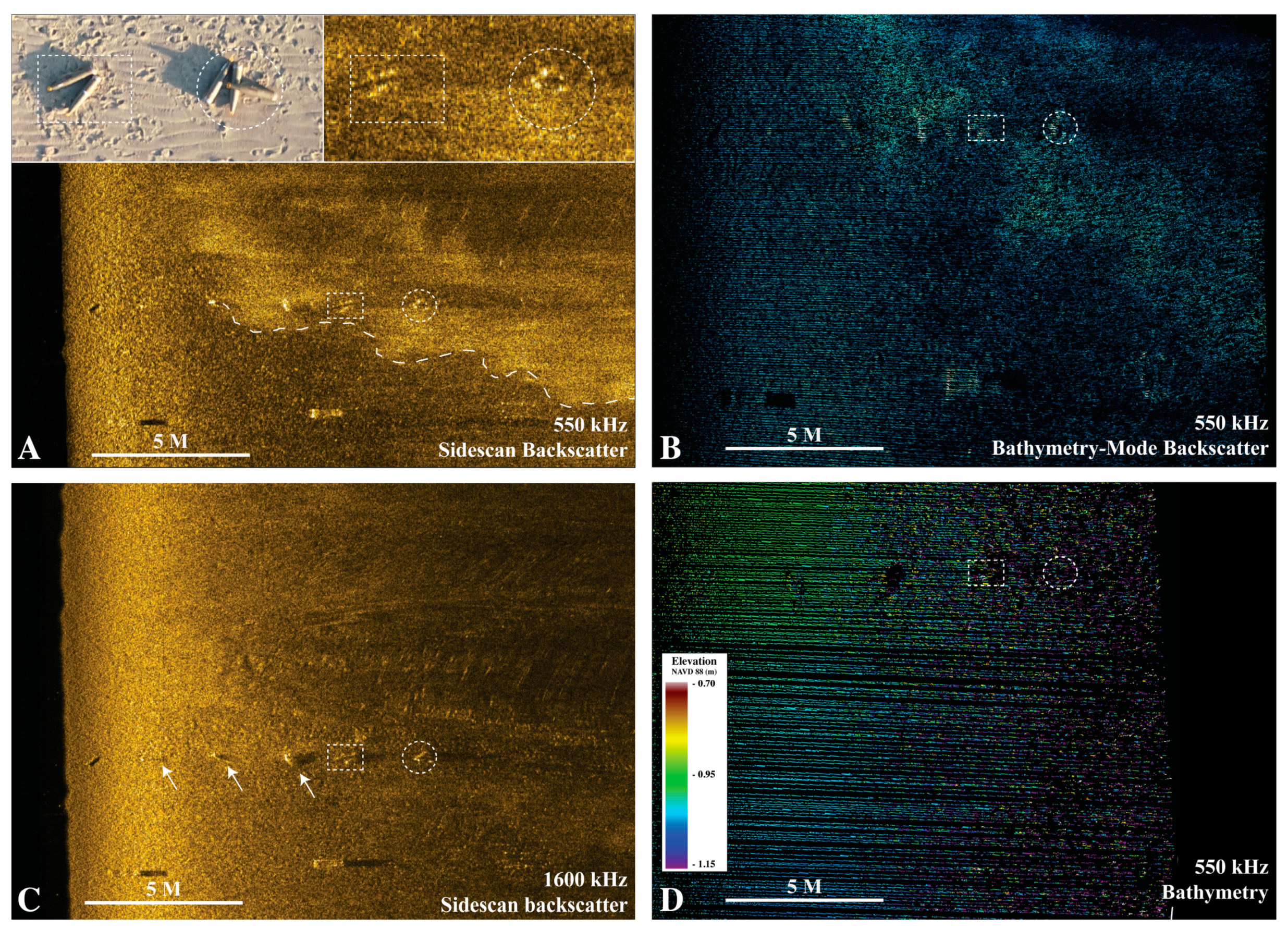
2.3.1. Sidescan Backscatter

The JSF files were imported into SonarWiz where a combination of automated and manual data processing was undertaken, including bottom tracking, slant range correction, offset entry, and gain setting adjustments. After appropriate processing of each data file, mosaics were generated, which were then exported in a raster format (Geotiffs). In order to create acoustic centroids from the sidescan backscatter data to compare with the GPS centroids, either end of each target in individual sonar files was assigned a 2-dimensional point in the digitizer window in SonarWiz. Objects are often blurred in sonar imagery, and the ends of a target adjacent to a homogenous seafloor can be easier to locate. In addition, similar to the GPS data, two points on either end of a linear target will provide the orientation of the target, which can then be used for DCL and the quantification of uncertainties based on attributes discussed below. Thus, centroids derived from the acoustic data are calculated by selecting a midpoint between chosen end points for a given target. The creation of the centroid generates a 2D data point (easting and northing) along with other optional information based on the sidescan backscatter, such as ping number, survey time, vessel heading and speed, range from nadir to target, water depth, and attitude of sonar (heave, pitch, and roll). Only targets that were clearly seen (detected) and identifiable (classified) in the acoustic data (e.g., sidescan backscatter, bathymetry or bathymetry-mode backscatter) were used to generate acoustic centroids. Detection or classification was not based on the GPS centroids or GPS-end points.

To calculate the accuracy of the location of the target based on the sidescan data, the acoustic centroid was compared to the GPS centroid. Summary statistics were produced (mean ± standard deviation (min–max)) based on acoustic channel (port or starboard), distance from nadir (0–20 m), and sidescan backscatter frequency (550 or 1600 kHz). In addition, linear models were produced to document how changes in motion parameters (heave, pitch, and roll) affect the localization of targets. These analyses were performed using R version 3.6 utilizing package “ggplot2” [43,44].

2.3.2. Bathymetry

Patch tests were performed in the field to determine motion and timing offsets (roll, pitch, yaw, and latency). Those offsets were recorded in the vessel file and applied when the survey lines were merged. Total propagated uncertainty (TPU) was computed using device manufacturer specifications recorded in the vessel configuration file.

The Edgetech 6205 collects bathymetry in two ways, as binned or raw, stave, data. The former collects data as directed by the operator, based on a user-specified bin size, bin size based on nadir depth, or specified angle binning [45], while the latter saves 9 simultaneous phase difference measurements on each channel (port/starboard) of the returning acoustic pulse. Each data point requires measurement across two of the 10 receiving staves (or piezoelectric elements) per channel [46]. Although this typically increases data storage that needs to be 5 times that of the default setting for binned data, it allows for troubleshooting and the ability to reprocess the data using different parameters and filters. It should be noted that saving data as binned or stave data has no impact on the sidescan backscatter, as a single stave acts as a ‘true sidescan’ with a single transducer emitting the acoustic ping and receiving the returning echo. The raw Edgetech files, stave JSF, were converted to standard JSF files using Discover Bathymetric (v 41). The conversion was performed using the no binning option, which is available in the bin size option mentioned above. It retains the maximum resolution of data possible in the cross-track direction. Additionally, the default engineering parameters and advanced bathymetric control was used, which rejects measurements that fail the quality control algorithm [45].

The JSF files were imported into CARIS (v 11.4.9) and the soundings were corrected using vessel and sensor offsets. The sound speed velocity profiles were applied using the nearest in time selection method. The tidal correction used the RTK tide exported from Hypack 2019 (v 1.19), smoothed by a 300 s fast Fourier transform low pass filter to eliminate high frequency oscillations. No vertical or horizontal datum transformation was applied.

Given the differences between sidescan or BMB and that of bathymetric data, a different method to determine the centroid was needed. Using the CARIS subset editor tool, a single operator analyzed each line individually, aiming to define the spatial limits of targets of interest. To delineate targets on the seafloor, a rainbow colormap was manually adjusted to highlight soundings using the 2D profile viewer tool. Once the objects were distinguished from the seabed on the 3D viewer, using the cursor circular selection tool, the operator marked a central point of interest and expanded a radius, which selected a small point cloud that contained all possible candidates, to the points of the targets. Those soundings were flagged and exported as vector files. Within a GIS, each cluster of points was associated with the closest GPS measurement, and the image from the UAS survey was used to confirm the most likely representation of the target. Special attention was given to locations where multiple targets existed. The orientation and aspect ratio of the candidate points were fixed, and the point clouds were moved horizontally to match the closest location of the GPS measurements. After associating the names of each sounding to the most likely GPS measurement, its original horizontal location was restored.

The results explored the soundings distances from the GPS measurements on the horizontal plane. The median value was extracted for each point cloud that shared the same label and compared with the GPS measurements. For each target, a centroid was computed using the half of the Euclidian distance between the two endpoints. If only one endpoint was found for a target, a second endpoint was estimated based on the GPS coordinates.

2.3.3. Bathymetry-Mode Backscatter (BMB)

The analysis of the reflectively backscatter shares techniques with the above-mentioned sidescan backscatter and bathymetric data. For the localization analysis, stave JSF files were processed through Discover Bathymetric in the same manner as the bathymetric data discussed above. Then, unlike the bathymetry data, the JSF files were imported into SonarWiz 7 (SW7) as bathymetric files using the import bathymetry files function. Once imported, the data were georeferenced using the merge function to account for vessel parameter offsets as well as sound velocity profiles taken during the survey. This allows for the most accurate geolocation of the individual soundings. There were no applications of filters, empirical gain normalization (EGN), or other manipulation of the data.

Once properly georeferenced, the acoustic data were displayed by bathymetry-mode backscatter amplitude (dB) in SonarWiz using a color ramp that allows for the efficient differentiation of objects from the seafloor. The scale of this color ramp was adjusted by the operator to allow for the best visual representation of these objects, typically focusing the color ramp around the 75–100 dB range. The RTK-GPS points taken at each survey site prior to the acoustic survey were then imported into SW7 to help the operator in the detection of objects.

Similar to the sidescan backscatter, the two ends of each target from sites 1 and 2 were selected using singular points visible in the dataset. These points were selected based on the amplitude of the BMB as well as adjacent acoustic shadows that would be indicative of objects proud of the seabed. Once all points for objects visible in the BMB were selected, they were exported as a .csv, containing point name and XY location. For each object on a per-line basis, the X and Y values for the two ends of targets were averaged to generate a centroid point. This calculated centroid was then compared to the centroid point of the RTK-GPS locations. All centroids were compared to the nearest GPS centroid using the near tool in ArcMap.

3. Results

At both sites, the targets were seeded at the first low tide of the day. Positional data were collected for the targets and the UAS survey as noted above. Approximately 2 h before the following high tide, the vessel-based surveys began. All surveys collected co-located sidescan sonar imagery, or sidescan backscatter, swath bathymetry, and non-calibrated BMB (Figure 3). Surveys were continued until sufficient data were collected to fully map the targets from survey lines of multiple orientations, achieve full coverage of the survey area, and provide satisfactory overlap of acoustic lines. Site 1 was a small intertidal flat that allowed for surveying from multiple directions. In order to collect data along the mixed sand and gravel bottom of Site 2, the intertidal zone along the beach could only be mapped with alongshore survey lines that could be safely navigated.

Site 1 was surveyed on 2 October 2020, Site 2 on 20 August 2020. On both days, winds were below 10 knots, with negligible wave heights and tidal currents of little impact as surveys were conducted at or near high tide. The low energy conditions were corroborated as little to no movement of the targets was observed in the intertidal (Figure 2A). At Site 1, 40 targets, 10 of each caliber, were placed in individual lines. For each line, five individual targets were placed in multiple orientations and five were set in two additional groups of two and three targets, resulting in seven locations where targets were positioned for each caliber for a total of twenty-eight locations. Individuals and groups were spaced approximately 1 m apart. Site 2 had a narrow, intertidal zone that had sufficient pebbles and cobbles to provide a suitable test of the method. Twelve targets, three of each caliber, were deployed in the intertidal zone roughly north to south from the largest to the smallest caliber.

3.1. UAS Data

Site 1 was flown at an altitude of 31 m above ground level (AGL) with a flight speed of 3.1 m/s and collected 197 images over the 23 min flight. Site 2 was flown at 45 m AGL with a flight speed of 3.1 m/s and collected 255 images over a 12 min flight (

Table 1. Alt AGL = Altitude above ground level, GCP = Ground control points, AA = Accuracy assessment.

	Images	Alt AGL (m)	GCPs	AA Points
Site 1	197	31	8	3
Site 2	255	45	5	5

).

The datasets used to perform the UAS localization were the orthomosaic and the DSM. Both datasets were loaded into ArcMap 10.7. A new shapefile was created, and the endpoints from the RTK-GPS survey were imported into the project GIS. Site 1 and 2 contained a total of 80 and 24 target end points, respectively. The easting and northing (x, y) coordinates were extracted from the mosaic, and the elevation (z coordinate) was extracted from the DSM. A comparison of each coordinate direction was made between the GPS points marked in the field and the points marked in the UAS-derived orthomosaic, so the difference and root mean square error (RMSE) could be computed.

RMSE measures the difference between where a map says a point is, and where the point is actually located. It is written as follows:

$$\mathrm{RMSE}=\sqrt{\frac{{\sum }_{i=1}^n{\left(P_i-O_i\right)}^2}{n}}$$

(1)

where P_i is the predicted value (model output) for the ith observation, O_i is the observed accuracy assessment point (GPS points), and n is the number of accuracy assessment points. Therefore, lower RMSE values indicate less distance between the UAS-derived location and the RTK-GPS-derived location, and thus are more accurate than those with higher RMSE values. After processing, both UAS flights yielded dense point clouds and accurate, high-resolution DSMs and orthomosaics (

Table 2. Results of the SfM processing from the Pix4D software. In this table, RMSE_x,y,z are the accuracy assessments calculated from points not used in the georeferencing of the point cloud. GSD and RMSE numbers are in cm.

	Date	Area (ha)	Points	Point Density (m3)	GSD	RMSEx	RMSEy	RMSEz
Site 1	2 October 2020	1.39	10,087,712	7199	0.81	3.6	1.7	2.2
Site 2	23 August 2020	9.78	17,651,328	677	1.83	2.9	1.7	1.2

) to be used in the localization analysis.

The localization results based on a comparison of the field collected target GPS points for site 1 were slightly different than those generated by the software in Table 2 with RMSEs of 2.0 cm, 1.6 cm, and 4.3 cm for the x, y, z coordinates, respectively. Site 2 results were 3.9 cm, 3.0 cm, and 3.9 cm, respectively, for the x, y, and z coordinates.

3.2. Vessel-Based Acoustic Data

The Site 1 survey included 89 survey lines, 12.23 km in length, collected over 2 h at or near high tide. The majority of survey lines mapped the area seeded with targets. Surveys at Site 2 include a total of 15 lines for 5.9 km for approximately 1 h at or near high tide. A total of seven of the fifteen lines were close enough to the intertidal zone to have mapped the targets. The range was set at 20 m, yielding a 40 m swath at both sites.

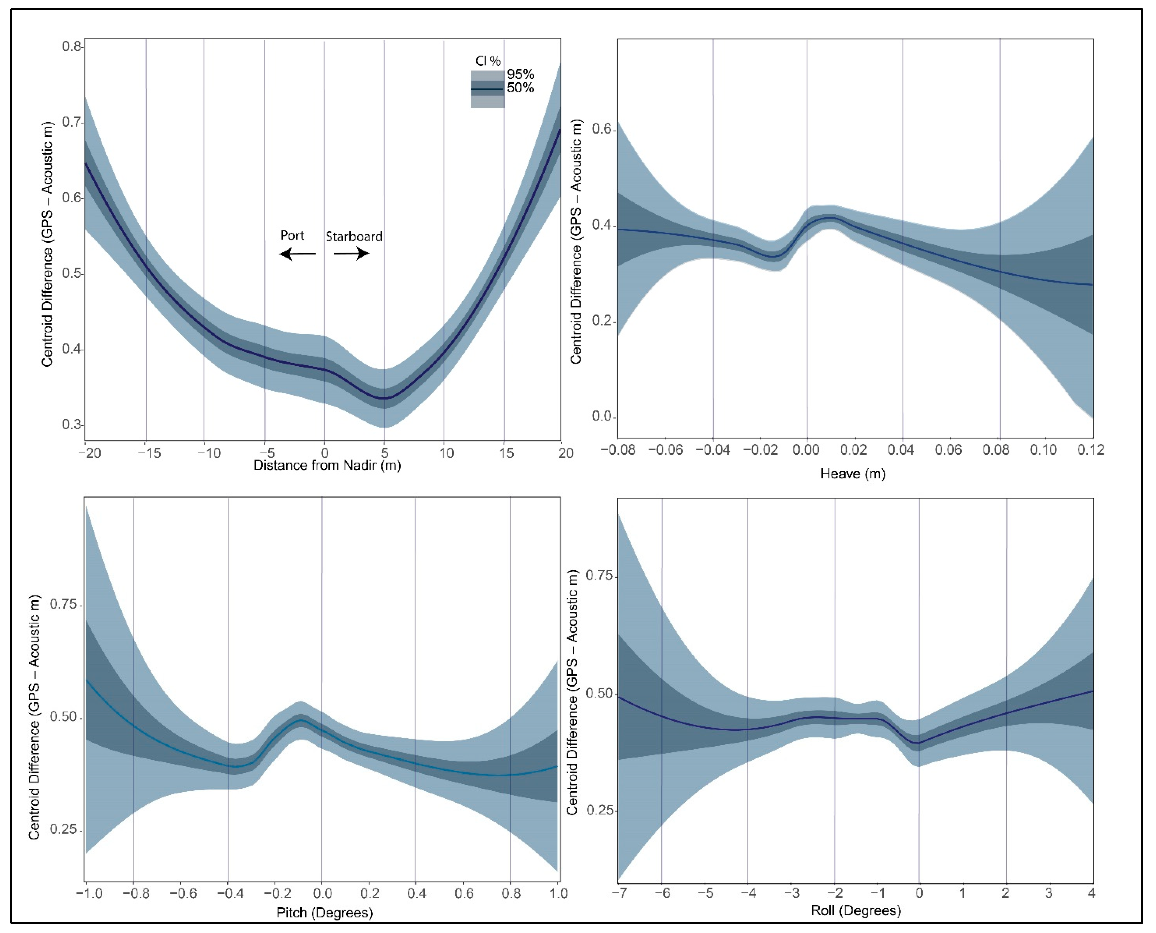
3.2.1. Sidescan Backscatter: Accuracy of Absolute Localization and Sources of Uncertainty

Centroids were created for all objects seen in the sidescan backscatter data. A total of 578 calls were identified in the 550 kHz imagery and 848 in the 1600 kHz imagery for a total of 1426 calls used for analysis. At Site 1, individual and groups of targets (n = 28) were each identified between 4 to 34 times in the 550 kHz data and 6 to 47 times in the 1600 kHz data. The group of three 155 mm targets were found more often than the group of two 155 mm targets, and individual targets whose long axes were parallel to survey lines were identified more than other orientations, and the larger objects (155 mm, n = 218) were found more than the smaller objects (60 mm, n = 88) (

Table 3. Positional uncertainty. Summary statistics for Site 1 (Provincetown Harbor) and Site 2 (Duck Harbor beach) surveys. Data for each object (mean ± standard deviation (min–max)) for both port and starboard and each frequency are indicated. Unless otherwise specified, units are in meters.

		Object	Port	Starboard	Both Sides
Site 1 (Provincetown Harbor)	550 kHz	60 mm	0.43 ± 0.26 (0.03–1.09) n = 47	0.44 ± 0.23 (0.04–0.87) n = 41	0.43 ± 0.24 (0.04–1.09) n = 88
		81 mm	0.45 ± 0.44 (0.09–2.38) n = 58	0.39 ± 0.28 (0.04–1.62) n = 45	0.43 ± 0.38 (0.04–2.38) n = 103
		105 mm	0.43 ± 0.27 (0.07–1.59) n = 82	0.48 ± 0.23 (0.07–1.21) n = 87	0.45 ± 0.25 (0.07–1.59) n = 169
		155 mm	0.52 ± 0.35 (0.05–1.7) n = 94	0.41 ± 0.24 (0.01–1.55) n = 124	0.46 ± 0.29 (0.01–1.7) n = 218
		550 kHz	0.46 ± 0.34 (0.03–2.38) n = 281	0.43 ± 0.24 (0.01–1.62) n = 297	0.45 ± 0.29 (0.01–2.38) n = 578
	1600 kHz	60 mm	0.3 ± 0.28 (0.01–1.09) n = 75	0.39 ± 0.23 (0.04–1.01) n = 56	0.34 ± 0.26 (0.01–1.09) n = 131
		81 mm	0.28 ± 0.19 (0.01–0.87) n = 82	0.36 ± 0.23 (0.02–0.9) n = 64	0.32 ± 0.21 (0.01–0.9) n = 146
		105 mm	0.33 ± 0.26 (0.02–1.37) n = 117	0.44 ± 0.24 (0.03–1) n = 140	0.39 ± 0.25 (0.02–1.37) n = 257
		155 mm	0.46 ± 0.33 (0.03–1.7) n = 152	0.41 ± 0.25 (0.02–1.29) n = 162	0.44 ± 0.29 (0.02–1.7) n = 314
		1600 kHz	0.36 ± 0.29 (0.01–1.7) n = 426	0.41 ± 0.24 (0.02–1.29) n = 422	0.39 ± 0.27 (0.01–1.7) n = 848
		TOTAL	0.4 ± 0.31 (0.01–2.38) n = 707	0.42 ± 0.24 (0.01–1.62) n = 719	0.41 ± 0.28 (0.01–2.385) n = 1426
Site 2 (Duck Harbor Beach)	550 kHz	60 mm	0.65 ± 0.51 (0.24–1.29) n = 5	0.61 ± 0.2 (0.47–0.75) n = 2	0.64 ± 0.42 (0.24–1.291) n = 7
		81 mm	0.38 ± 0.18 (0.2–0.69) n = 5	0.61 ± - (0.61–0.61) n = 1	0.42 ± 0.19 (0.2–0.692) n = 6
		105 mm	0.4 ± 0.23 (0.1–0.7) n = 5	0.29 ± 0.25 (0.1–0.58) n = 3	0.36 ± 0.23 (0.1–0.696) n = 8
		155 mm	0.37 ± 0.25 (0.13–0.65) n = 5	0.27 ± 0.11 (0.14–0.39) n = 4	0.33 ± 0.2 (0.13–0.654) n = 9
		550 kHz	0.45 ± 0.32 (0.1–1.29) n = 20	0.38 ± 0.22 (0.1–0.75) n = 10	0.43 ± 0.29 (0.1–1.291) n = 30
	1600 kHz	60 mm	0.45 ± 0.29 (0.16–1.02) n = 8	0.31 ± 0.17 (0.09–0.45) n = 4	0.41 ± 0.26 (0.09–1.021) n = 12
		81 mm	0.43 ± 0.25 (0.17–0.99) n = 9	0.42 ± 0.17 (0.21–0.62) n = 5	0.42 ± 0.22 (0.17–0.989) n = 14
		105 mm	0.38 ± 0.19 (0.09–0.68) n = 9	0.41 ± 0.18 (0.18–0.73) n = 7	0.39 ± 0.18 (0.09–0.726) n = 16
		155 mm	0.47 ± 0.36 (0.14–1.26) n = 9	0.24 ± 0.18 (0.03–0.48) n = 7	0.37 ± 0.31 (0.03–1.263) n = 16
		1600 kHz	0.43 ± 0.27 (0.09–1.26) n = 35	0.34 ± 0.18 (0.03–0.73) n = 23	0.4 ± 0.24 (0.03–1.263) n = 58
		TOTAL	0.44 ± 0.28 (0.09–1.29) n = 55	0.35 ± 0.19 (0.03–0.75) n = 33	0.41 ± 0.25 (0.03–1.291) n = 88

).

Overall, the accuracy for Site 1 was 0.41 ± 0.28 m (0.01–2.385 m), (mean ± standard deviation (min–max); though the accuracy for Site 2 was the same as Site 1, the standard deviation and range were different, 0.41 ± 0.25 m (0.03–1.291 m) (Table 3). The sonar channel (port v starboard) affected localization in the 1600 kHz data with the port channel being slightly more accurate (0.36 ± 0.29 m (0.01–1.7 m) than the starboard channel (0.41 ± 0.24 m (0.02–1.29 m) (p = 0.004 *, t test). However, the two frequencies were not significantly different from each other (p = 0.2649, t test) (Table 3). Differences in accuracy between the 550 and 1600 are likely due to the higher pixel resolution of the 1600 frequency, allowing for a more precise localization of the object.

The distance of the target from nadir was a significant source of variability with regard to positional uncertainty (Figure 4). The highest uncertainties occurred at both extremes, near nadir and at the edges of the sonagram. (

Table 4. Summary statistics for both frequencies (550 and 1600 kHz) from the Provincetown Harbor survey across the swath range (0–20 m). Data for distance bin (mean ± standard deviation (min–max)) for both port and starboard and each frequency are displayed. All units are in meters.

550 kHz				1600 kHz
Range (m)	Port	Starboard	Total	Port	Starboard	Total
0	-	0.59 ± 0.19 (0.36–1.1) n = 12	0.59 ± 0.19 (0.36–1.1) n = 12	0.91 ± (0.91–0.91) n = 1	0.62 ± 0.2 (0.3–1) n = 13	0.64 ± 0.2 (0.3–1) n = 14
1	0.53 ± 0.23 (0.24–0.85) n = 8	0.3 ± 0.08 (0.24–0.36) n = 2	0.49 ± 0.23 (0.24–0.85) n = 10	0.54 ± 0.28 (0.28–1.01) n = 10	0.39 ± 0.1 (0.28–0.47) n = 3	0.51 ± 0.26 (0.28–1.01) n = 13
2	0.37 ± 0.19 (0.09–0.71) n = 9	0.36 ± 0.16 (0.05–0.6) n = 8	0.37 ± 0.17 (0.05–0.71) n = 17	0.49 ± 0.3 (0.16–1.23) n = 13	0.47 ± 0.26 (0.18–0.99) n = 10	0.48 ± 0.28 (0.16–1.23) n = 23
3	0.4 ± 0.2 (0.17–0.76) n = 15	0.15 ± 0.13 (0.04–0.43) n = 7	0.32 ± 0.22 (0.04–0.76) n = 22	0.48 ± 0.26 (0.12–1.04) n = 17	0.32 ± 0.29 (0.02–0.92) n = 15	0.41 ± 0.29 (0.02–1.04) n = 32
4	0.46 ± 0.38 (0.06–1.32) n = 20	0.27 ± 0.2 (0.04–0.87) n = 21	0.36 ± 0.31 (0.04–1.32) n = 41	0.41 ± 0.33 (0.03–1.37) n = 21	0.25 ± 0.21 (0.08–0.81) n = 19	0.34 ± 0.29 (0.03–1.37) n = 40
5	0.47 ± 0.27 (0.08–1.09) n = 21	0.25 ± 0.14 (0.03–0.62) n = 19	0.37 ± 0.24 (0.03–1.09) n = 40	0.44 ± 0.26 (0.01–1.08) n = 29	0.23 ± 0.18 (0.03–0.77) n = 29	0.33 ± 0.25 (0.01–1.08) n = 58
6	0.36 ± 0.23 (0.09–0.86) n = 12	0.3 ± 0.12 (0.12–0.64) n = 27	0.32 ± 0.16 (0.09–0.86) n = 39	0.37 ± 0.25 (0.06–1.03) n = 15	0.28 ± 0.2 (0.07–0.71) n = 34	0.31 ± 0.21 (0.06–1.03) n = 49
7	0.29 ± 0.2 (0.05–0.98) n = 29	0.32 ± 0.16 (0.01–0.66) n = 27	0.31 ± 0.18 (0.01–0.98) n = 56	0.34 ± 0.24 (0.01–1.04) n = 35	0.26 ± 0.18 (0.02–0.89) n = 41	0.29 ± 0.21 (0.01–1.04) n = 76
8	0.34 ± 0.26 (0.12–1.09) n = 18	0.39 ± 0.27 (0.11–1.21) n = 19	0.37 ± 0.26 (0.11–1.21) n = 37	0.37 ± 0.25 (0.06–1.08) n = 24	0.31 ± 0.14 (0.09–0.59) n = 22	0.34 ± 0.2 (0.06–1.08) n = 46
9	0.39 ± 0.28 (0.03–1.04) n = 17	0.42 ± 0.2 (0.13–0.76) n = 20	0.41 ± 0.24 (0.03–1.04) n = 37	0.34 ± 0.24 (0.03–0.91) n = 24	0.33 ± 0.18 (0.06–0.85) n = 32	0.33 ± 0.2 (0.03–0.91) n = 56
10	0.38 ± 0.39 (0.05–1.1) n = 9	0.37 ± 0.11 (0.21–0.54) n = 7	0.38 ± 0.29 (0.05–1.1) n = 16	0.38 ± 0.34 (0.03–1.35) n = 23	0.35 ± 0.16 (0.08–0.64) n = 15	0.37 ± 0.28 (0.03–1.35) n = 38
11	0.61 ± 0.39 (0.22–1.31) n = 7	0.44 ± 0.16 (0.17–0.71) n = 13	0.5 ± 0.27 (0.17–1.31) n = 20	0.39 ± 0.38 (0.07–1.23) n = 16	0.36 ± 0.18 (0.04–0.83) n = 28	0.37 ± 0.27 (0.04–1.23) n = 44
12	0.37 ± 0.34 (0.09–1.34) n = 11	0.39 ± 0.1 (0.18–0.49) n = 8	0.38 ± 0.26 (0.09–1.34) n = 19	0.4 ± 0.32 (0.04–1.37) n = 21	0.38 ± 0.1 (0.21–0.7) n = 21	0.39 ± 0.23 (0.04–1.37) n = 42
13	0.6 ± 0.48 (0.22–1.85) n = 10	0.59 ± 0.35 (0.1–1.62) n = 13	0.59 ± 0.4 (0.1–1.85) n = 23	0.35 ± 0.23 (0.06–0.87) n = 18	0.48 ± 0.18 (0.12–0.72) n = 14	0.41 ± 0.22 (0.06–0.87) n = 32
14	0.52 ± 0.33 (0.19–1.4) n = 15	0.57 ± 0.13 (0.34–0.71) n = 6	0.54 ± 0.28 (0.19–1.4) n = 21	0.3 ± 0.28 (0.06–1.32) n = 33	0.54 ± 0.14 (0.29–0.77) n = 15	0.38 ± 0.27 (0.06–1.32) n = 48
15	0.65 ± 0.49 (0.26–2.22) n = 16	0.54 ± 0.23 (0.04–0.95) n = 14	0.6 ± 0.39 (0.04–2.22) n = 30	0.27 ± 0.32 (0.02–1.41) n = 20	0.54 ± 0.23 (0.18–0.96) n = 23	0.42 ± 0.31 (0.02–1.41) n = 43
16	0.53 ± 0.3 (0.22–1.63) n = 19	0.55 ± 0.21 (0.16–1.01) n = 25	0.54 ± 0.25 (0.16–1.63) n = 44	0.29 ± 0.3 (0.06–1.58) n = 29	0.57 ± 0.15 (0.22–0.85) n = 30	0.43 ± 0.27 (0.06–1.58) n = 59
17	0.62 ± 0.46 (0.24–2.38) n = 24	0.55 ± 0.19 (0.13–0.89) n = 22	0.59 ± 0.36 (0.13–2.38) n = 46	0.29 ± 0.25 (0.02–1.19) n = 39	0.61 ± 0.19 (0.25–1.01) n = 30	0.43 ± 0.28 (0.02–1.19) n = 69
18	0.54 ± 0.34 (0.26–1.7) n = 14	0.53 ± 0.23 (0.18–0.94) n = 14	0.54 ± 0.29 (0.18–1.7) n = 28	0.36 ± 0.38 (0.04–1.7) n = 24	0.69 ± 0.21 (0.23–1.05) n = 18	0.5 ± 0.36 (0.04–1.7) n = 42
19	0.5 ± 0.15 (0.3–0.69) n = 6	0.57 ± 0.24 (0.23–0.87) n = 9	0.54 ± 0.2 (0.23–0.87) n = 15	0.29 ± 0.19 (0.11–0.8) n = 14	0.64 ± 0.33 (0.1–1.1) n = 6	0.39 ± 0.29 (0.1–1.1) n = 20
20	0.67 ± (0.67–0.67) n = 1	1.1 ± 0.31 (0.8–1.55) n = 4	1.02 ± 0.33 (0.67–1.55) n = 5		0.9 ± 0.39 (0.4–1.29) n = 4	0.9 ± 0.39 (0.4–1.29) n = 4
550	0.46 ± 0.34 (0.03–2.38) n = 281	0.43 ± 0.24 (0.01–1.62) n = 297	0.45 ± 0.29 (0.01–2.38) n = 578	0.36 ± 0.29 (0.01–1.7) n = 426	0.41 ± 0.24 (0.02–1.29) n = 422	0.39 ± 0.27 (0.01–1.7) n = 848

). Data between 3–7 m from nadir had the lowest uncertainty for each sonar channel and for both frequencies (Table 4).

Motion of the vessel also contributes to the positional uncertainty. A linear model for heave, pitch, and roll was created, as expected, that greater positional uncertainties are directly related to increases in vessel motion (Figure 4). It should be noted that these surveys were conducted in very shallow waters, during optimal sea state conditions; therefore, this information should not be used to infer positional uncertainties during poor conditions. However, it is informative to observe the contributions to positional uncertainty from minor changes in vessel attitude.

3.2.2. Bathymetry and Bathymetry-Mode Backscatter: Accuracy of Absolute Localization

For the analysis of the bathymetric data at Site 1, ten lines of acoustic were used, five each approximately perpendicular and parallel to shoreline orientation. Water depths during the survey varied from 1.87 m to 2.53 m. At Site 2, five survey lines were used, all parallel to the shoreline in both directions. The water depths during the survey varied from 1.95 m to 2.78 m. Of the three data types used here, the bathymetric data proved to have been the least effective method of detecting and classifying the targets, even though localization was similar to other data types.

At Site 1 for the ten lines of acoustic data, 104 calls were made. Overall, the accuracy for Site 1 was 0.18 ± 0.14 m (0.02–1.00 m), (mean ± standard deviation (min–max). At Site 2, from the five lines used, eighteen calls of targets were made, yielding an accuracy of 0.14 ± 0.09 m (0.02–0.38 m).

For the BMB data at Site 1, all 28 target locations were visible as stated above, the groups of two and three were treated as one target. Within the 10 lines of data, 149 calls were made. For Site 2, using five lines, only nine of the twelve objects were detectable, and only eighteen calls were made on the nine targets. For Site 1, the average linear distance between the BMB centroids and the centroids calculated from RTK-GPS points was 0.15 ± 0.10 m (0.01–0.51 m), (mean ± standard deviation (min–max). For Site 2, the average linear distance between the GPS centroids and the acoustic centroids was 0.13 ± 0.09 m (0.01–0.35 m).

4. Discussion

The improvements to the localization of targets along the seafloor is critical to many applications and the techniques discussed herein can aid similar types of investigations where precise geographic positioning is needed. The relationship between distance from nadir and the quality of acoustic data, or ‘sweet spot’, will not be surprising to those in the field; however, the quantification of the absolute location of targets within these datasets will be of aid to all users of the data, rather than anecdotal or often-quoted conventional wisdom for such values.

The uncertainty of the absolute localization of targets was independent of bottom type. The standard deviation of sandy intertidal areas, Site 1, vs. mixed sand and gravel (largely cobble bottom) Site 2 was 0.255 m and 0.279 m, respectively. The detection and classification of targets were significantly more challenging at Site 2, but once detected, the acoustic data were well-suited to quantify the absolute localization of the targets.

The sidescan backscatter range was set to 20 m for all surveys in this study and results show that 98.9% of all targets ensonified were mapped <1 m away from their absolute location (Figure 5) or within the uncertainty needed for remedial action for UXO [7]. In fact, more that two-thirds of the targets were within 0.5 m of their absolute location and 25% were under 0.25 m.

When needed, after identifying a target or targets of interest, hydrographers can re-position future survey lines to ensure a near nadir pass, enabling the most accurate localization values. For example, our findings show that targets between 3–7 m from nadir have the least amount of uncertainty with regard to absolute location. In the case of UXO remediation, it should be done prior to divers or equipment being sent to the seafloor. Safety protocols for shallow water surveys, such as ensonifying the seafloor prior to placing the vessel above that stretch of seafloor, will allow the hydrographer to visualize and avoid any potential navigation hazards [28]. This technique is most critical when working with UXO or other munitions.

While some studies use the MBES as a comparison point to gauge the quality of other systems, including PMSSs [35], we believe it is inherent upon investigators to improve our quantification of the absolute localization of targets or features on the seafloor. The quality of MBESs has long been known [29], but a unique standard to compare all targets from positional acoustic data is needed. Techniques used in this study are useful for very shallow waters, but more work is needed for deeper waters.

While PMSSs have limitations [34,35], there are also opportunities with these instruments for advancements in the field due to their utility in shallow water environments and the nature of the co-located bathymetry and backscatter data products. There is a type of redundancy that can be useful when time-sensitive work in hazardous areas is being conducted. Figure 3A,C show the effects of air bubbles in the water column as a result of prop wash; this interference is not seen in the bathymetry or the higher sidescan backscatter frequency. These types of verification that do not add to survey times and yet reduce uncertainties with regard to the absence/presence of targets or features on the seafloor can be invaluable.

Practically, for work with proud UXO, this study has shown that in very shallow waters (0–3 m) the localization threshold for remediation can be achieved with acoustic data only, using the sensors and platforms discussed here and following the methods and techniques outlined above. However, much work needs to be carried out. Other acoustic sensors with similar resolution and platforms able to deliver those instruments should be able to produce similar results seen here. Future work could involve a series of analyses to improve detection to reduce the false positives to zero. Some hypotheses to be tested could include: after the detection of munitions, X number of calls within 3–7 m of nadir on different survey lines will functionally decrease the false positives to zero; after X ensonifications of the target with its long axis parallel to the sonar, the false positives will functionally decrease to zero; and the first two hypotheses designed for detections can also improve the quality of the classification and localization of the ensonified targets.

It should be noted that, while the accuracy for the localization of the targets using bathymetric data was slightly better than in the sidescan or BMB, it is very likely that this was due to only the larger targets being observable in the bathymetric data. Despite the fact that GPS centroids are available to the operator if the target was not clearly discernible in the data, no acoustic endpoints were selected.

5. Conclusions

The absolute localization of targets or features on the seafloor using acoustic instruments can be critical to multiple types of investigations. The use of a PMSS can provide the resolution and bottom coverage of a high frequency sidescan sonar with the positional accuracy of a vessel-mounted MBES. The co-located datasets can also be advantageous in hazardous areas where human safety is at risk, providing multiple types of data in one survey. This study focused on surveys in two bottom types, sandy and predominantly cobble, and found that the accuracy of absolute localization was relatively independent of bottom type, although detection was more difficult along cobble bottoms. With high numbers of target calls (n = 1426), an accuracy of 0.41 ± 0.26 m was seen in the sidescan backscatter, with distance from nadir being the most significant source of uncertainty. Targets imaged between 3–7 m from nadir had the lowest uncertainty with an increase toward and away from nadir. Although vessel motion (heave, pitch, and roll) is typically a contributing factor, it was much less so here, largely due to surveys being conducted during very favorable conditions, which minimized overall motion.

The phase-measuring sidescan sonar used in the study yielded three data types and sidescan backscatter was the preferred dataset for the DCL of targets. Bathymetry and BMB were less useful for detection and classification, but once the accuracy of absolute localization was detected, they were similar to that of sidescan backscatter. Due to the fewer lines used for the subset analysis, the calls of targets for bathymetry and BMB were 122 and 139, respectively, an order of magnitude less than those from sidescan backscatter. These findings were included in this study to demonstrate the utility of these co-located datasets.

References

1. Alevizos, E.; Snellen, M.; Simons, D.; Siemes, K.; Greinert, J. Multi-angle backscatter classification and sub-bottom profiling for improved seafloor characterization. Mar. Geophys. Res. 2017, 39, 289–306. [Google Scholar] [CrossRef]
2. Gumusay, M.U.; Bakirman, T.; Kizilkaya, I.T.; Aykut, N.O. A review of seagrass detection, mapping and monitoring applications using acoustic systems. Eur. J. Remote Sens. 2018, 52, 1–29. [Google Scholar] [CrossRef] [Green Version]
3. Herkül, K.; Peterson, A.; Paekivi, S. Applying multibeam sonar and mathematical modeling for mapping seabed substrate and biota of offshore shallows. Estuarine Coast. Shelf Sci. 2017, 192, 57–71. [Google Scholar] [CrossRef]
4. LaFrance, M.; King, J.W.; Oakley, B.A.; Pratt, S. A comparison of top-down and bottom-up approaches to benthic habitat mapping to inform offshore wind energy development. Cont. Shelf Res. 2014, 83, 24–44. [Google Scholar] [CrossRef]
5. Madricardo, F.; Ghezzo, M.; Nesto, N.; Mc Kiver, W.J.; Faussone, G.C.; Fiorin, R.; Riccato, F.; Mackelworth, P.C.; Basta, J.; De Pascalis, F.; et al. How to Deal with Seafloor Marine Litter: An Overview of the State-of-the-Art and Future Perspectives. Front. Mar. Sci. 2020, 7, 830. [Google Scholar] [CrossRef]
6. Misiuk, B.; Brown, C.J. Multiple imputation of multibeam angular response data for high resolution full coverage seabed mapping. Mar. Geophys. Res. 2022, 43, 1–20. [Google Scholar] [CrossRef]
7. Richardson, M.; Nelson, H.; Williams, K.; Calantoni, J. SERDP/ESTCP munitions response program: Underwater remediation of unexploded ordnance (UXO). In Proceeding of the Underwater Acoustics Conference and Exhibition (UACE), Hersonissos, Greece, 8–12 July 2019. [Google Scholar]
8. Wehner, D.; Frey, T. Offshore Unexploded Ordnance Detection and Data Quality Control—A Guideline. IEEE J. Sel. Top. Appl. Earth Obs. Remote Sens. 2022, 15, 7483–7498. [Google Scholar] [CrossRef]
9. Etter, D.; Delaney, B. Report of the Defense Science Board Task Force on Unexploded Ordnance; Defense Science Board: Washington, DC, USA, 2003. [Google Scholar] [CrossRef]
10. SERDP-ESTCP. Munitions in the Underwater Environment: State of the Science and Knowledge, Strategic Environmental Research and Development Program (SERDP); Environmental Security Technology Certification Program (ESTCP): Washington, DC, USA, 2010. [Google Scholar]
11. Hożyń, S. A Review of Underwater Mine Detection and Classification in Sonar Imagery. Electronics 2021, 10, 2943. [Google Scholar] [CrossRef]
12. Brown, D.C.; Johnson, S.F.; Gerg, I.D.; Brownstead, C.F. Simulation and testing results for a sub-bottom imaging sonar. In Proceedings of Meetings on Acoustics 178ASA; Acoustical Society of America: San Diego, CA, USA, 2019; p. 070001. [Google Scholar]
13. Hansen, R.E. Mapping the ocean floor in extreme resolution using interferometric synthetic aperture sonar. Proc. Meet. Acoust. Acoust. Soc. Am. 2019, 38, 055003. [Google Scholar] [CrossRef] [Green Version]
14. Keenan, S.T.; Clark, D.; Blay, K.R.; Leslie, K.; Foley, C.P.; Billings, S. Calibration and testing of a HTS tensor gradiometer for underwater UXO detection. In Proceedings of the 2011 International Conference on Applied Superconductivity and Electromagnetic Devices, Sydney, NSW, Australia, 14–16 December 2011; IEEE: Sydney, NSW, Australia, 2011; pp. 135–137. [Google Scholar]
15. Marston, T.M.; Williams, A.T.; Plotnick, D.S. Sub-aperture recombination for sliding window SAS processing in 3D down-looking synthetic aperture sonar, EUSAR 2021. In Proceedings of the 13th European Conference on Synthetic Aperture Radar, Online, 29 March–1 April 2021; pp. 1–6. [Google Scholar]
16. Yu, Y.; Zhao, J.; Gong, Q.; Huang, C.; Zheng, G.; Ma, J. Real-Time Underwater Maritime Object Detection in Side-Scan Sonar Images Based on Transformer-YOLOv5. Remote Sens. 2021, 13, 3555. [Google Scholar] [CrossRef]
17. Yulin, T.; Jin, S.; Bian, G.; Zhang, Y. Shipwreck Target Recognition in Side-Scan Sonar Images by Improved YOLOv3 Model Based on Transfer Learning. IEEE Access 2020, 8, 173450–173460. [Google Scholar] [CrossRef]
18. Jerram, K.; Schmidt, V. Storm Response Surveying with Phase-Measuring Bathymetric Sidescan Sonar; Center for Coastal and Ocean Mapping, UNH: Durham, NH, USA, 2015; p. 20. [Google Scholar]
19. Trembanis, A.; DuVal, C.; Beaudoin, J.; Schmidt, V.; Miller, D.; Mayer, L. A detailed seabed signature from Hurricane Sandy revealed in bedforms and scour. Geochem. Geophys. Geosystems 2013, 14, 4334–4340. [Google Scholar] [CrossRef] [Green Version]
20. Borrelli, M.; Fox, S.E.; Shumchenia, E.J.; Kennedy, C.G.; Oakley, B.A.; Hubeny, J.B.; Love, H.; Smith, T.L.; Legare, B.; Mittermayr, A.; et al. Submerged Marine Habitat Mapping, Cape Cod National Seashore: A Post-Hurricane Sandy Study; Natural Resource Report NPS/NCBN/NRR—2019/1877; National Park Service: Fort Collins, CO, USA, 2019. [Google Scholar] [CrossRef]
21. Grouthues, T.M.; Levin, D.; Psuty, N.P.; Habeck, A.; Petrecca, R.; Dobarro, J. Submerged Marine Habitat Mapping at Sandy Hook Unit, Gateway National Recreation Area: A Post-Hurricane Sandy Study; Natural Resource Report NPS/NCBN/NRR—2019/1865; National Park Service: Fort Collins, CO, USA, 2019. [Google Scholar]
22. Bartley, M.L.; King, J.W.; Oakley, B.A.; Caccioppoli, B.J. Post-Hurricane Sandy Benthic Habitat Mapping at Fire Island National Seashore, New York, USA, Utilizing the Coastal and Marine Ecological Classification Standard (CMECS). Estuaries Coasts 2022, 45, 1070–1094. [Google Scholar] [CrossRef]
23. Mittermayr, A.; Legare, B.; Borrelli, M. Applications of the Coastal and Marine Ecological Classification Standard (CMECS) in a Partially Restored New England Salt Marsh Lagoon. Estuaries Coasts 2020, 45, 1095–1106. [Google Scholar] [CrossRef]
24. Mittermayr, A.; Legare, B.J.; Kennedy, C.G.; Fox, S.E.; Borrelli, M. Using CMECS to Create Benthic Habitat Maps for Pleasant Bay, Cape Cod, Massachusetts. Northeast. Nat. 2020, 27, 22. [Google Scholar] [CrossRef]
25. Trembanis, A.C.; Miller, D.C.; Ebula, E.; Rusch, H.M.; Rothermel, E.R. Submerged Marine Habitat Mapping at Assateague Island National Seashore: A Post-Hurricane Sandy Study; Natural Resource Report NPS/NCBN/NRR—2019/1871; National Park Service: Fort Collins, CO, USA, 2019. [Google Scholar]
26. Legare, B.; Mittermayr, A.; Borrelli, M. The impacts of hydraulic clamming in shallow water and the importance of incorporating anthropogenic disturbances into habitat assessments. Aquat. Living Resour. 2020, 33, 13. [Google Scholar] [CrossRef]
27. Legare, B.J.; Nichols, O.C.; Borrelli, M. Persistence of Hydraulic Dredge Tracks Following Surfclam Harvesting in Shallow Water. J. Shellfish. Res. 2020, 39, 331–336. [Google Scholar] [CrossRef]
28. Borrelli, M.; Smith, T.L.; Mague, S.T. Vessel-Based, Shallow Water Mapping with a Phase-Measuring Sidescan Sonar. Estuaries Coasts 2021, 45, 961–979. [Google Scholar] [CrossRef]
29. Hughes Clarke, J.E. Multibeam Echosounders, Submarine Geomorphology; Springer Geology: Cham, Switzerland, 2018; pp. 25–41. [Google Scholar]
30. Mayer, L.A.; Raymond, R.; Glang, G.; Richardson, M.D.; Traykovski, P.; Trembanis, A.C. High-Resolution Mapping of Mines and Ripples at the Martha’s Vineyard Coastal Observatory. IEEE J. Ocean. Eng. 2007, 32, 133–149. [Google Scholar] [CrossRef] [Green Version]
31. Wolfson, M.L.; Naar, D.F.; Howd, P.A.; Locker, S.D.; Donahue, B.T.; Friedrichs, C.T.; Trembanis, A.C.; Richardson, M.D.; Wever, T.F. Multibeam Observations of Mine Burial Near Clearwater, FL, Including Comparisons to Predictions of Wave-Induced Burial. IEEE J. Ocean. Eng. 2007, 32, 103–118. [Google Scholar] [CrossRef]
32. Grall, P.; Kochanska, I.; Marszal, J. Direction-of-Arrival Estimation Methods in Interferometric Echo Sounding. Sensors 2020, 20, 3556. [Google Scholar] [CrossRef]
33. Grall, P.; Marszal, J. Method for the correlation coefficient estimation of the bottom echo signal in the shallow water application using interferometric echo sounder. Vib. Phys. Syst. 2021, 32. [Google Scholar]
34. Mohammadloo, T.H.; Geen, M.; SSewada, J.; Snellen, M.; GSimons, D. Assessing the Performance of the Phase Difference Bathymetric Sonar Depth Uncertainty Prediction Model. Remote Sens. 2022, 14, 2011. [Google Scholar] [CrossRef]
35. Pimentel, L.V.; Florentino, L.C.; Neto, A. Evaluation of the Precision of Phase-Measuring Bathymetric Side Scan Sonar Relative to Multibeam Echosounders. Int. Hydrogr. Rev. 2020, 24, 61–83. [Google Scholar]
36. McCormack, B.; Borrelli, M. Shallow Water Object Detection, Characterization, and Localization Through Uncalibrated Reflectivity Backscatter from a Phase-Measuring Sidescan. in preprint.
37. dos Santos, P.P.G.M.; Borrelli, M. Estimating Absolute Positional Uncertainties Associated with Bathymetric Data from a Phase-Measuring Sidescan Sonar in Very Shallow Waters. in preprint.
38. Uchupi, E.; Giese, G.; Aubrey, D.; Kim, D. The late quaternary construction of Cape Cod, Massachusetts: A reconsideration of the WM Davis model. Geol. Soc. Am. Spec. Pap. 1996, 309, 1–69. [Google Scholar]
39. Zeigler, J.M.; Tuttle, S.D.; Tasha, H.J.; Giese, G.S. The Age and Development of The Provincelands Hook, Outer Cape Cod, Massachusetts. Limnol. Oceanogr. 1965, 10, R298–R311. [Google Scholar] [CrossRef]
40. Portman, M.E.; Jin, D.; Thunberg, E. The connection between fisheries resources and spatial land use change: The case of two New England fish ports. Land Use Policy 2011, 28, 523–533. [Google Scholar] [CrossRef]
41. Oldale, R.N.; O’Hara, C.J. Glaciotectonic origin of the Massachusetts coastal end moraines and a fluctuating late Wisconsinan ice margin. Geol. Soc. Am. Bull. 1984, 95, 61–74. [Google Scholar] [CrossRef]
42. James, M.R.; Robson, S. Straightforward reconstruction of 3D surfaces and topography with a camera: Accuracy and geoscience application. J. Geophys. Res. Earth Surf. 2012, 117, 03017. [Google Scholar] [CrossRef] [Green Version]
43. R Core Team. R: A Language and Environment for Statistical Computing; R Foundation for Statistical Computing: Vienna, Austria, 2019; Available online: https://www.R-project.org/ (accessed on 15 October 2022).
44. Wickham, H.; Chang, W.; Henry, L.; Pedersen, T.L.; Takahashi, K.; Wilke, C.; Woo, K.; Yutani, H.; Dunnington, D. Ggplot2: Create Elegant Data Visualisations Using the Grammar of Graphics; R Package Version; 2016; Volume 2. Available online: https://ggplot2.tidyverse.org/reference/ggplot2-package.html (accessed on 15 November 2022).
45. Edgetech. Discover Bathymetric: User Software Manual-0014878_REV_G. Date: 3/17/2022. 2022, p. 108. Available online: https://www.edgetech.com/wp-content/uploads/2019/07/0014878_Rev_H.pdf (accessed on 15 November 2022).
46. Brisson, L.N.; Wolfe, D.A.; Matthew Staley, P.S.M. Interferometric Swath Bathymetry for Large Scale Shallow Water Hydrographic Surveys. In Canadian Hydrographic Conference; Canadian Hydrographic Association: St. John’s, NL, Canada, 2014; p. 18. Available online: https://www.edgetech.com/wp-content/uploads/2019/07/EdgeTech-Paper-on-6205-presented-at-CHC2014.pdf (accessed on 15 November 2022).
Figure 1. (Left) Site 1: sandy intertidal area in Provincetown Harbor. Inset locus map. (Right) Site 2: mixed sand and gravel beaches with predominantly cobble bottom. Yellow boxes are approximate locations of surveys.
Remotesensing 15 01626 g001
Figure 2. Intertidal survey areas. (A) Site 1, a sandy intertidal flat with a group of three 155 mm, wax-filled mortar shells. This group underwent no observable movement between one LT-HT-LT cycle based on RTK-GPS measurements. (B) Site 2, a mixed sand and gravel beach with many cobble-sized material. A single 155 mm, wax-filled mortar shell. (C) Site 2, horizontal sidescan data over the UAS imagery. Note the alignment of the second from the bottom target in both datasets. The bedforms in the lower left exhibit 12–15 cm spacing. (D) Site 2, vertical sidescan overlay over UAS imagery. Note the shadows in the lower two targets seen in the sidescan data.
Remotesensing 15 01626 g002
Figure 3. Starboard channel of the four data types from a phase-measuring sidescan sonar from Site 1, a sandy intertidal flat. (A) Raw, low frequency sidescan backscatter, black vertical bar to left of image is ‘water column’ from sidescan waterfall. Note the dashed line, highlighting a different bottom reflector also seen in (B), but not (C) or (D). Upper left inset is from UAS image. Upper right inset is zoom of rectangle and circle from waterfall below. (B) Bathymetry-mode backscatter. (C) Raw, high frequency sidescan backscatter. (D) Swath bathymetry, note the bottom coverage is not as extensive away from nadir.
Remotesensing 15 01626 g003
Figure 4. Absolute localization and sources for uncertainty for all sidescan backscatter data. (Upper left) distance from nadir. (Upper right) Heave in meters. (Lower left) Pitch in degree. (Lower right) Roll in degrees. CI = Confidence interval.
Remotesensing 15 01626 g004
Figure 5. Difference between the GPS centroid and acoustic centroid in 10 cm bins for all acoustic data types (n = 1867). sB = sidescan backscatter (550 kHz, n = 578; 1600 kHz, n = 848), BMB (change figure inset) = bathymetry-mode backscatter (n = 139), Bathymetry (n = 122).
Remotesensing 15 01626 g005