

Reasoning-Based Scheduling Method for Agile Earth Observation Satellite with Multi-Subsystem Coupling

Abstract
:1. Introduction
- A satellite coupling state prediction method was proposed. We analyzed the coupling relationship between satellite observation, data transmission, and electricity subsystems. Subsequently, we determined the different coupling states of AEOS with each subsystem as the main limiting factor and sorted the variables that reflected the satellite coupling states, and then proposed a state prediction method for these variables;
- RS was established. Based on the observation-priority scheduling strategy in previous research [34,35], we proposed two planning strategies including the data transmission-priority scheduling strategy and electricity-priority scheduling strategy. We also constructed reasoning rules that corresponded to different scheduling strategies for different satellite coupling states.
2. Problem Description
- represents the decision of whether to observe target i;
- represents whether the observation of target j is after the observation of target i or not;
- represents whether to download the observation data of target i or not;
- represents whether the download mission of target j is after the observation of target i or not.
3. Proposed Methods
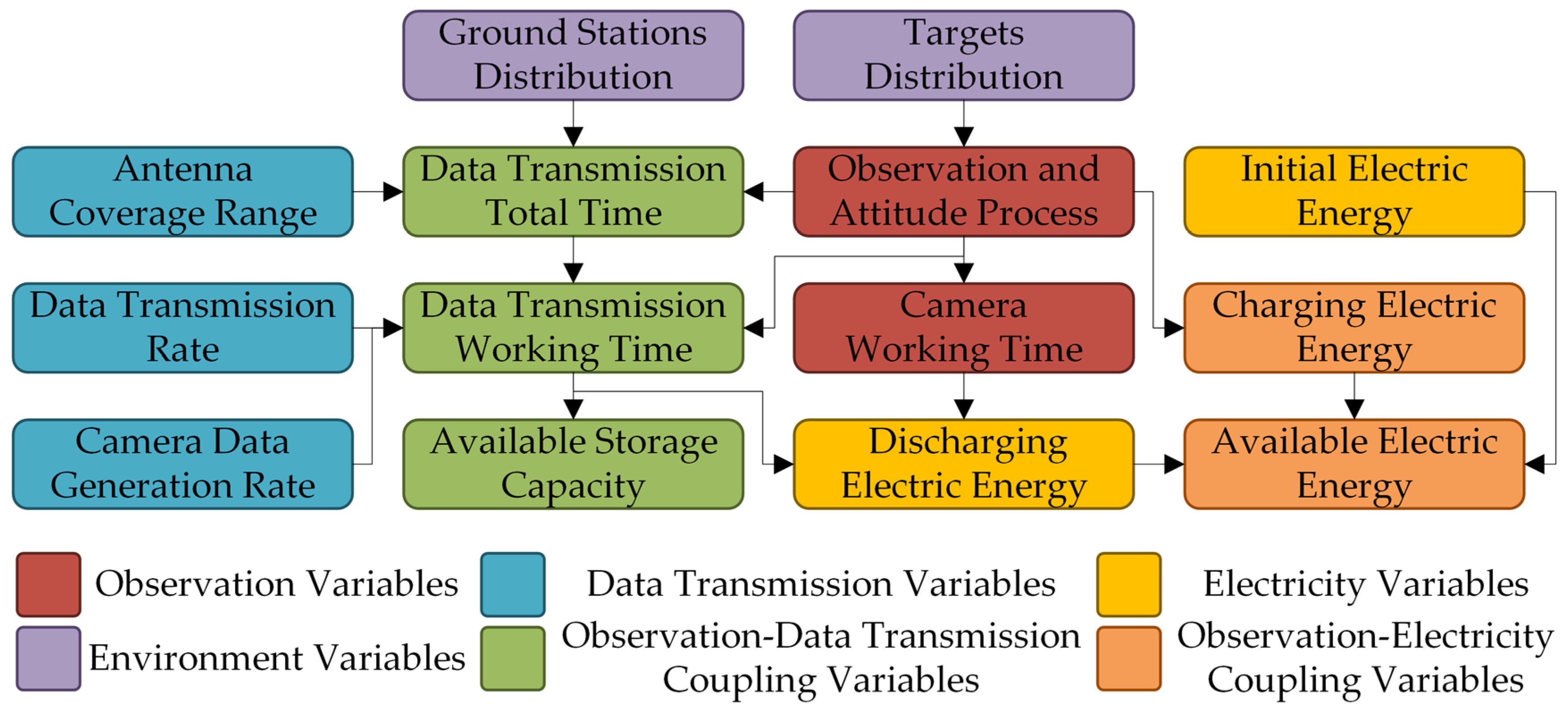
- The coupling relationship between the satellite observation, data transmission, and electricity subsystems is analyzed. Next, the different coupling states where each subsystem is the main limiting factor are identified, followed by the extraction of the coupling characteristic variables reflecting different coupling states;
- The description of the RS algorithm including the satellite state prediction, reasoning of the target selection strategies, target weight calculation, target selection, and scheduling;
- Three heuristic scheduling methods are given on the basis of three scheduling strategies for a comparison with RS.
3.1. Multi-Subsystems Coupling Relationship Analysis of Earth Observation Satellite
3.2. Reasoning-Based Scheduling Method
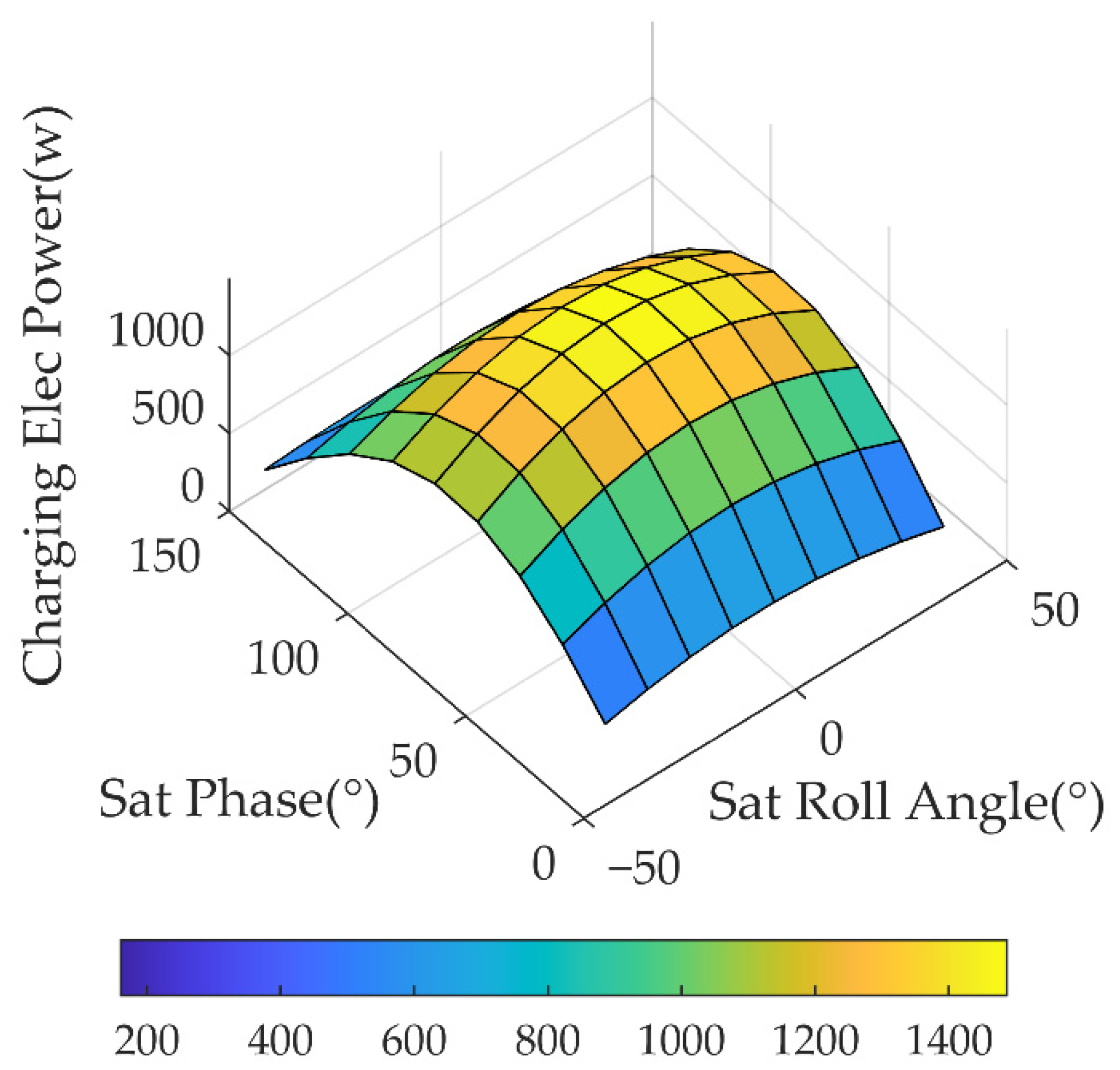
3.2.1. Satellite State Prediction
3.2.2. Rule-Based Reasoning and Target Weight Calculation
- IF OR
- THEN
- IF AND
- THEN
- IF
- THEN
- IF
- THEN
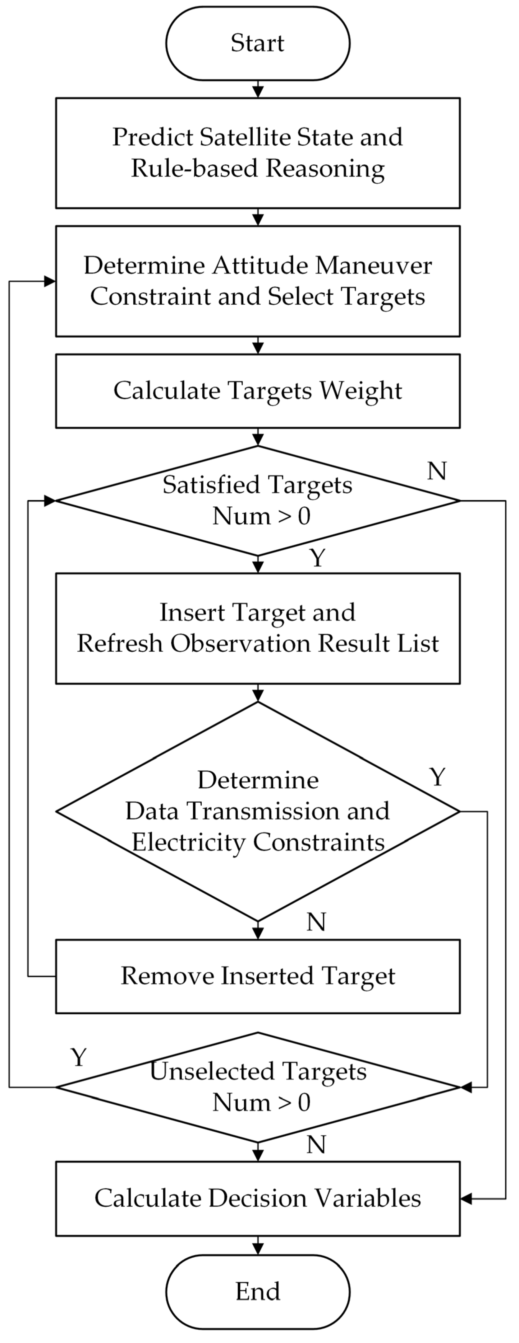
3.2.3. Targets Selecting and Scheduling
- Predict the satellite states according to the method mentioned in Section 3.1, and calculate the preferred flag of targets using rule-based reasoning according to the method mentioned in Section 3.2;
- Unselected targets form a set . Determine whether the sequence satisfies the attitude maneuver constraint after each unselected target is inserted at the position of the maximum sequence’s backward time slack. Subsequently, select targets that satisfy the attitude maneuver constraint and form a target set that satisfy the attitude constraint . The attitude maneuver constraint is stated in Equation (3), and the calculation of the insertion position of the maximum backward time slack is included in Appendix C;
- Calculate the weights of targets in according to Equation (22);
- If the number of targets in is more than 0, go to step 5, otherwise, go to step 9;
- Take out the target with the highest weight in and insert it into the current observation sequence at the maximum sequence’s backward time slack position. Then, update the target observation sequence and remove the selected target from ;
- Based on the target observation sequence, calculate the satellite’s attitude, data transmission time windows, the data downloading time, occupied memory capacity, and available electrical energy, the calculation method of the satellite state can be found in Appendix B;
- Determine whether the data transmission constraints and electricity constraint are satisfied according to Equations (4)–(9). If the observation sequence does not satisfy the constraints after inserting the target, remove the target from the observation sequence and go to step 4, otherwise, go to step 8;
- If the number of unselected targets in is more than 0, return to step 2, else, go to step 9;
- The observation sequence contains the information of and . According to and , calculate other decision variables and parameters including , , , and using the calculation method mentioned in Appendix B.
3.3. Heuristic Scheduling Methods
4. Simulation Results
5. Discussion
- A potential direction is to apply the method to more different conditions, with the purpose of supplementing the knowledge base in the reasoning process according to the simulation results, and modifying the parameters;
- Simulations can be carried out on a finer-grained component level that is closer to a real satellite. This includes the operation simulation for different satellite components, the simulation of observation data generation and transmission, and the simulation of the power consuming processes of the components. According to a finer-grained simulation condition, the simulation results can be utilized to improve the scheduling algorithm;
- Research can be conducted on mission allocation and resource distribution for multiple satellites and orbits. Scheduling on more orbits will bring target observation opportunities in different orbit periods, reduce the pressure of observation and data transmission missions on a single orbit by selecting targets in different orbits, and hence obtain more profits. It is also crucial to perform research on how to coordinate limited resources among multiple satellites to obtain better multi-satellite mission scheduling results;
- Targets can be merged in the preprocessing step. When the field of view of the satellite’s camera is relatively wider and the distances between targets are shorter, multiple targets can be observed with a single observation. If this merging preprocess needs to be integrated into our proposed method, the neighboring targets are required to be grouped according to their satellite orbits and the frame widths of the camera in the target preprocessing step. The roll angle, time window, and scanning time duration also need to be calculated so that these grouped targets can be added to the methodological framework proposed in this paper.
6. Conclusions
Author Contributions
Funding
Data Availability Statement
Acknowledgments
Conflicts of Interest
Appendix A. Time Window Calculation Method
Appendix B. Decision Variables Calculation Method
- Calculate the satellite’s attitude progress based on the current satellite observation target scheduling result list. Then, calculate the start time and end time of the data transmission time windows, and sort the data transmission time windows according to start time . Attitude progress can be calculated as follows:where is the satellite attitude maneuver angle calculation function. The satellite attitude angle can be calculated using the current attitude angle, target attitude angle, and a calculating time (i.e., it can be a moment during attitude maneuver or after attitude maneuver is completed). Earth-pointing mode is the operation mode when there is no mission. If the time between the current observation mission and next observation mission is not enough for the satellite to turn to the Earth-pointing attitude and then turn to the next target observation attitude, the satellite will then maintain the attitude for a set period of time before maneuvering to the next target observation attitude. If the time between the current observation mission and the next observation mission is enough to turn to the Earth-pointing attitude and then turn to the next target observation attitude, the satellite will first turn to the Earth-pointing attitude, and maintain the attitude for a certain time, and then turn to the observation attitude of the next target;
- Select an observation target according to the order of the observation result sequence. Targets are categorized into selected targets and unselected targets according to and , and the observation target sort sequence is the sequence of the selected target serial numbers sorted according to the order of observation targets , where is the number of selected targets, and is the serial number of a target;
- Start with k = 1, then select the kth data transmission time window and calculate the available time segment of the data transmission time window that satisfies the data transmission constraints, which can be expressed aswhere and are the start time and end time of the occupied segment of the data transmission time window k.
- Determine whether the available time segment of the kth data transmission time window is sufficient for downloading the observation data of target . If there is enough time, the data transmission start time is the start time . Otherwise, set k = k + 1, and repeat the calculation of the available time segment and download the time judgement. If there is not enough time for data downloading in all of the data transmission time windows, the data transmission constraints are not satisfied. Hence, the data transmission time calculation is ended;
- Repeat Steps 2 to 4 until the data download time calculation of all the observation targets are completed. The targets’ observation data download time can be calculated and the data transmission constraints can be judged at the same time.
Appendix C. Maximum Backward Time Slack Heuristic Scheduling Method
- Calculate the backward time slack of each target. For a target sequence (i, …, j), the backward time slack of the observation of target i is the time that i can move backward without violating the observation time window constraint and the attitude maneuver constraint, which can be calculated by the back-forward iteration as
- The sequence’s backward time slack is the minimum backward time of all selected targets, which can be defined as
- where sequence . Calculate the backward time slack of target i after target i is inserted at position p, which is
- where is the observation end time after target i is inserted into position p. Insertion position p is defined as the position where an unselected target i, between the selected target p and p + 1, is inserted. After target i is inserted into position p, the start time of observation mission p + 1 in the original sequence becomes
- The sequence’s backward time slack after target i is inserted into position p is ;
- 2.
- Determine whether the observation result sequence satisfies the attitude maneuver constraint after inserting an unselected target into the maximum sequence’s backward time slack position. Subsequently, select the targets that satisfy the attitude maneuver constraint after the insertion. If the number of satisfied targets is more than 0, go to step 3, otherwise the calculation is finished;
- 3.
- Select target i and insertion position p that allows the sequence to obtain the maximum sequence’s backward time slack after insertion. Insert target i at position p, update the observation result sequence, and remove target i from the unselected target set;
- 4.
- If the number of unselected targets is more than 0, return to step 1, otherwise the calculation is finished.
References
- Zhang, B.; Wu, Y.; Zhao, B.; Chanussot, J.; Hong, D.; Yao, J.; Gao, L. Progress and Challenges in Intelligent Remote Sensing Satellite Systems. IEEE J. Sel. Top. Appl. Earth Obs. Remote Sens. 2022, 15, 1814–1822. [Google Scholar] [CrossRef]
- Lin, M.S.; Jia, Y.J. Past, Present and Future Marine Microwave Satellite Missions in China. Remote Sens. 2022, 14, 16. [Google Scholar] [CrossRef]
- Dial, G.; Bowen, H.; Gerlach, F.; Grodecki, J.; Oleszczuk, R. IKONOS satellite, imagery, and products. Remote Sens. Environ. 2003, 88, 23–36. [Google Scholar] [CrossRef]
- Lamard, J.L.; Gaudin-Delrieu, C.; Valentini, D.; Renard, C.; Tournier, T.; Laherrere, J.M. Design of the high resolution optical instrument for the pleiades HR earth observation satellites. In Proceedings of the 5th International Conference on Space Optics (ICSO 2004), Toulouse, France, 30 March–2 July 2004; pp. 149–156. [Google Scholar]
- Gu, X.F.; Tong, X.D. Overview of China Earth Observation Satellite Programs. IEEE Geosci. Remote Sens. Mag. 2015, 3, 113–129. [Google Scholar] [CrossRef]
- Wang, J.J.; Song, G.P.; Liang, Z.; Demeulemeester, E.; Hu, X.J.; Liu, J. Unrelated parallel machine scheduling with multiple time windows: An application to earth observation satellite scheduling. Comput. Oper. Res. 2023, 149, 14. [Google Scholar] [CrossRef]
- Lemaitre, M.; Verfaillie, G.; Jouhaud, F.; Lachiver, J.M.; Bataille, N. Selecting and scheduling observations of agile satellites. Aerosp. Sci. Technol. 2002, 6, 367–381. [Google Scholar] [CrossRef]
- Peng, G.S.; Song, G.P.; Xing, L.N.; Gunawan, A.; Vansteenwegen, P. An Exact Algorithm for Agile Earth Observation Satellite Scheduling with Time-Dependent Profits. Comput. Oper. Res. 2020, 120, 15. [Google Scholar] [CrossRef]
- Zhang, B.; Chen, Z.; Peng, D.; Benediktsson, J.A.; Liu, B.; Zou, L.; Li, J.; Plaza, A. Remotely sensed big data: Evolution in model development for information extraction point of view. Proc. IEEE 2019, 107, 2294–2301. [Google Scholar] [CrossRef]
- Zhang, G.; Li, X.; Hu, G.; Zhang, Z.; An, J.; Man, W. Mission Planning Issues of Imaging Satellites: Summary, Discussion, and Prospects. Int. J. Aerosp. Eng. 2021, 2021, 7819105. [Google Scholar] [CrossRef]
- Xie, P.; Wang, H.; Chen, Y.; Wang, P. A Heuristic Algorithm Based on Temporal Conflict Network for Agile Earth Observing Satellite Scheduling Problem. IEEE Access 2019, 7, 61024–61033. [Google Scholar] [CrossRef]
- Grasset-Bourdel, R.; Flipo, A.; Verfaillie, G. Planning and replanning for a constellation of agile Earth observation satellites. In Proceedings of the 21th International Conference on Automated Planning and Scheduling (ICAPS 2011), Freiburg, Germany, 11–16 June 2011; p. 29. [Google Scholar]
- Wang, X.-W.; Chen, Z.; Han, C. Scheduling for single agile satellite, redundant targets problem using complex networks theory. Chaos Solitons Fractals 2016, 83, 125–132. [Google Scholar] [CrossRef]
- Wang, P.; Gao, P.; Tan, Y. A Model, a Heuristic and a Decision Support System to Solve the Earth Observing Satellites Fleet Scheduling Problem. In Proceedings of the International Conference on Computers and Industrial Engineering (CIE39), Troyes, France, 6–9 July 2009; pp. 256–261. [Google Scholar]
- Sun, H.; Xia, W.; Wang, Z.; Hu, X. Agile Earth Observation Satellite Scheduling Algorithm for Emergency Tasks Based on Multiple Strategies. J. Syst. Sci. Syst. Eng. 2021, 30, 626–646. [Google Scholar] [CrossRef]
- Liang, J.; Zhu, Y.H.; Luo, Y.Z.; Zhang, J.C.; Zhu, H. A precedence-rule-based heuristic for satellite onboard activity planning. Acta Astronaut. 2021, 178, 757–772. [Google Scholar] [CrossRef]
- Baek, S.-W.; Han, S.-M.; Cho, K.-R.; Lee, D.-W.; Yang, J.-S.; Bainum, P.M.; Kim, H.-D. Development of a scheduling algorithm and GUI for autonomous satellite missions. Acta Astronaut. 2011, 68, 1396–1402. [Google Scholar] [CrossRef]
- Liu, X.; Laporte, G.; Chen, Y.; He, R. An adaptive large neighborhood search metaheuristic for agile satellite scheduling with time-dependent transition time. Comput. Oper. Res. 2017, 86, 41–53. [Google Scholar] [CrossRef]
- Du, B.; Li, S.; She, Y.; Li, W.; Liao, H.; Wang, H. Area targets observation mission planning of agile satellite considering the drift angle constraint. J. Astron. Telesc. Instrum. Syst. 2018, 4, 047002. [Google Scholar] [CrossRef]
- Cui, K.; Xiang, J.; Zhang, Y. Mission planning optimization of video satellite for ground multi-object staring imaging. Adv. Space Res. 2018, 61, 1476–1489. [Google Scholar] [CrossRef]
- Hao, H.; Jiang, W.; Li, Y. Improved algorithms to plan missions for agile earth observation satellites. J. Syst. Eng. Electron. 2014, 25, 811–821. [Google Scholar] [CrossRef]
- Barkaoui, M.; Berger, J. A new hybrid genetic algorithm for the collection scheduling problem for a satellite constellation. J. Oper. Res. Soc. 2020, 71, 1390–1410. [Google Scholar] [CrossRef]
- Zhang, J.W.; Xing, L.N. An improved genetic algorithm for the integrated satellite imaging and data transmission scheduling problem. Comput. Oper. Res. 2022, 139, 11. [Google Scholar] [CrossRef]
- Zhou, Z.B.; Chen, E.M.; Wu, F.; Chang, Z.X.; Xing, L.N. Multi-satellite scheduling problem with marginal decreasing imaging duration: An improved adaptive ant colony algorithm. Comput. Ind. Eng. 2023, 176, 12. [Google Scholar] [CrossRef]
- Long, W.J. Medical informatics: Reasoning methods. Artif. Intell. Med. 2001, 23, 71–87. [Google Scholar] [CrossRef]
- Moulin, B.; Irandoust, H.; Belanger, M.; Desbordes, G. Explanation and argumentation capabilities: Towards the creation of more persuasive agents. Artif. Intell. Rev. 2002, 17, 169–222. [Google Scholar] [CrossRef]
- Gayathri, R.; Uma, V. Ontology based knowledge representation technique, domain modeling languages and planners for robotic path planning: A survey. ICT Express 2018, 4, 69–74. [Google Scholar] [CrossRef]
- Wu, X.J.; Tang, J.; Li, Q.; Heng, K.H. A vector-format fuzzy logic approach for online robot motion planning in 3D space and its application to underwater robotic vehicle. Robotica 2007, 25, 325–339. [Google Scholar] [CrossRef]
- Vilchis-Medina, J.-L.; Godary-Dejean, K.; Lesire, C. Autonomous Decision-Making With Incomplete Information and Safety Rules Based on Non-Monotonic Reasoning. IEEE Robot. Autom. Lett. 2021, 6, 8357–8362. [Google Scholar] [CrossRef]
- Martins, L.S.; Prajoux, R. Locomotion control of a four-legged robot embedding real-time reasoning in the force distribution. Robot. Auton. Syst. 2000, 32, 219–235. [Google Scholar] [CrossRef]
- Abiyev, R.H.; Akkaya, N.; Gunsel, I. Control of Omnidirectional Robot Using Z-Number-Based Fuzzy System. IEEE Trans. Syst. Man Cybern. -Syst. 2019, 49, 238–252. [Google Scholar] [CrossRef]
- Song, Y.; Xing, L.; Wang, M.; Yi, Y.; Xiang, W.; Zhang, Z. A knowledge-based evolutionary algorithm for relay satellite system mission scheduling problem. Comput. Ind. Eng. 2020, 150, 106830. [Google Scholar] [CrossRef]
- Tinker, P.; Fox, J.; Green, C.; Rome, D.; Casey, K.; Furmanski, C. Analogical and case-based reasoning for predicting satellite task schedulability. In Case-Based Reasoning Research and Development, Proceedings; MunozAvila, H., Ricci, F., Eds.; Lecture Notes in Artificial Intelligence; Springer-Verlag Berlin: Berlin, Germany, 2005; Volume 3620, pp. 566–578. [Google Scholar]
- Rojanasoonthon, S.; Bard, J. A GRASP for parallel machine scheduling with time windows. INFORMS J. Comput. 2005, 17, 32–51. [Google Scholar] [CrossRef] [Green Version]
- He, R. Research on Imaging Reconnaissance Satellite Scheduling Problem. Ph.D. Thesis, National University of Defense Technology, Changsha, China, 2004. [Google Scholar]
- Nanry, W.P.; Barnes, J.W. Solving the pickup and delivery problem with time windows using reactive tabu search. Transp. Res. Pt. B-Methodol. 2000, 34, 107–121. [Google Scholar] [CrossRef]
- Bloechliger, I.; Zufferey, N. A graph coloring heuristic using partial solutions and a reactive tabu scheme. Comput. Oper. Res. 2008, 35, 960–975. [Google Scholar] [CrossRef]
- Zhao, J.; Yang, F. Agile Satellite; National Defense Industry Press: Beijing, China, 2021. [Google Scholar]


| Parameter | Meaning |
|---|---|
| The number of targets | |
| The profit of target i | |
| , | The start and end time of the scheduling |
| The observation time of single target | |
| , | The start time and the end time of the observation of target i, the relationship between them is |
| The data transmission time of single target | |
| , | The start time and the end time of the data transmission of target i, the relationship between them is |
| The device switching time between each data transmission in different time windows | |
| The attitude maneuver time required for attitude transition of two observation missions | |
| , | The start time and the end time of the observation time window of target i |
| , | The start time and the end time of the data transmission time window k |
| M, | M is the occupied memory capacity and is the total memory capacity |
| W, | W is the available electrical energy and is the electrical energy capacity of the battery |
| Parameter Name | Parameter Value |
|---|---|
| Orbit Type | Sun-synchronous Orbit |
| Orbit Height | 650 km |
| Orbit Eccentricity | 0 |
| Orbit Inclination | 97.99° |
| Orbit Right Ascension of Ascending Node | 100.348° |
| Orbit Argument of Perigee | 0° |
| Attitude Maneuver Calculate Method | Trapezoidal Method |
| Max Attitude Maneuver Angular Velocity | 1°/s |
| Max Attitude Maneuver Angular Acceleration | 0.5°/s2 |
| Max Maneuvering Range Half Cone Angle | 45° |
| Camera’s Data Generation Rate | 2 Gbps |
| Data Transmission Rate | 1 Gbps |
| Antenna Coverage Half Cone Angle | 70° |
| Max Charging Electrical Power of Solar Arrays | 1.5 kW |
| Camera Electrical Power | 1 kW |
| Data Transmission Devices Electrical Power | 0.5 kW |
| Satellite Normal Electrical Power | 0.2 kW |
| Battery Electrical energy Capacity | 2.7 × 10⁶ J |
| Single Target Observation Time | 20 s |
| Parameter Name | Group 1 | Group 2 | Group 3 |
|---|---|---|---|
| Initial Electrical energy | 2 × 10⁶ J | 2 × 10⁶ J | 2 × 10⁵ J |
| Memory Capacity | 1200 Gbit | 1200 Gbit | 1200 Gbit |
| Target Number | 55 | 60 | 55 |
| Target Distribution Area Number | 2 | 3 | 2 |
| Target Number in Each Area | 15; 40 | 25; 15; 20 | 15; 40 |
| Sub-satellite Point Phase Range of Target Distribution (°) | [9.3, 62.1]; [9.3, 62.1] | [12.4, 55.9]; [12.4, 55.9]; [62.1, 99.3] | [62.1, 124.1]; [62.1, 124.1] |
| Angle Range between Targets and Orbital Plane (°) | [−0.5, 0.5]; [4.2, 6.2] | [−5.1, −2.1]; [2.1, 5.1]; [0, 2.1] | [−0.5, 0.5]; [4.2, 6.2] |
| Max Target Value | 1 | 1 | 1 |
| Min Target Value | 0.9 | 0.9 | 0.9 |
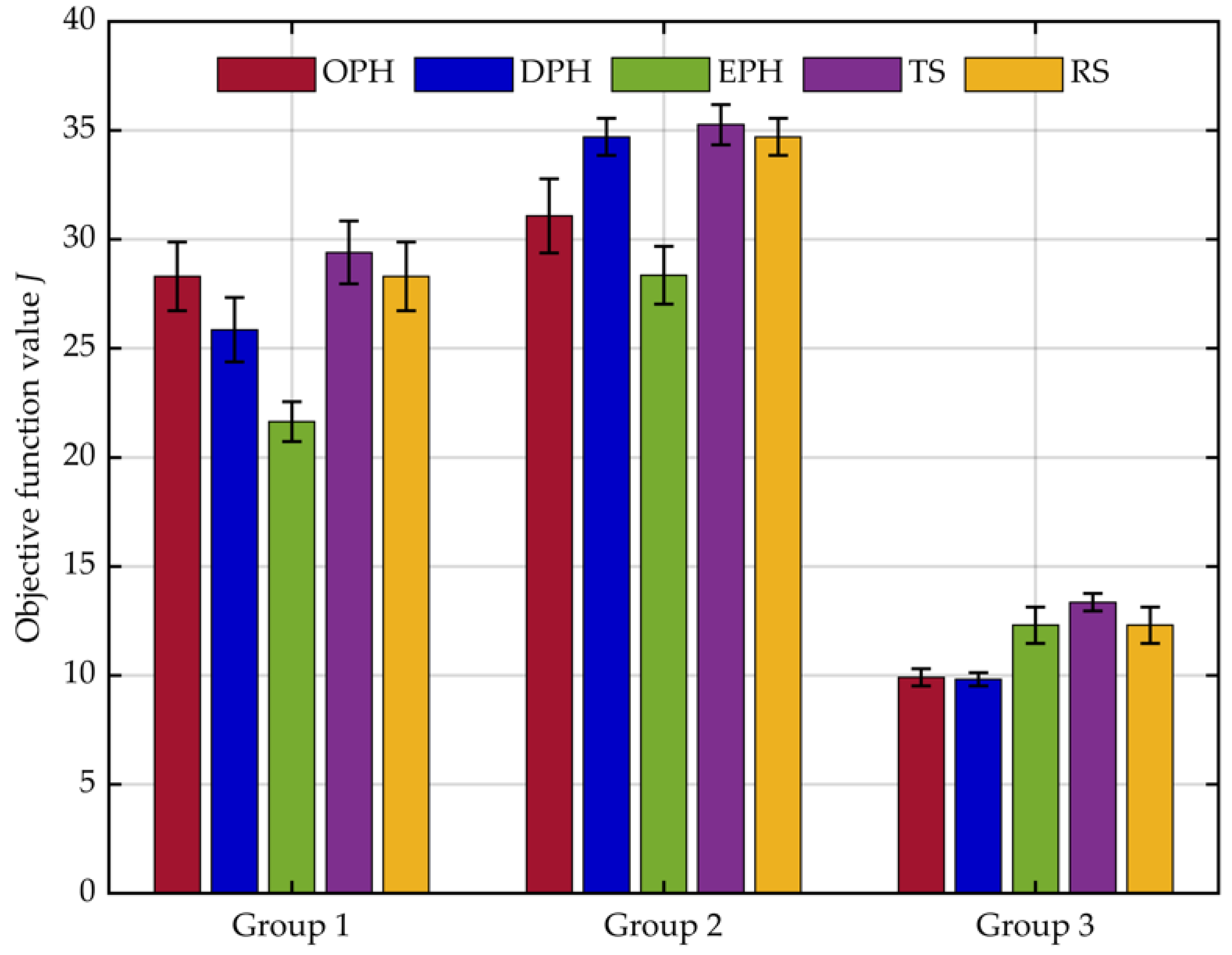
| Group 1 | Group 2 | Group 3 | |||||||
|---|---|---|---|---|---|---|---|---|---|
| Method | Max | Min | Avg | Max | Min | Avg | Max | Min | Avg |
| OPH [34,35] | 31.13 | 26.52 | 28.30 | 33.85 | 29.35 | 31.07 | 10.67 | 9.67 | 9.91 |
| EPH | 27.63 | 22.75 | 25.85 | 35.90 | 33.62 | 34.70 | 10.67 | 9.67 | 9.82 |
| DPH | 22.67 | 19.68 | 21.64 | 30.35 | 26.17 | 28.36 | 14.12 | 11.24 | 12.30 |
| TS [36,37] | 31.23 | 27.48 | 29.40 | 36.90 | 34.00 | 35.26 | 14.23 | 12.56 | 13.35 |
| RS | 31.13 | 26.52 | 28.30 | 35.90 | 33.62 | 34.70 | 14.12 | 11.24 | 12.30 |
Disclaimer/Publisher’s Note: The statements, opinions and data contained in all publications are solely those of the individual author(s) and contributor(s) and not of MDPI and/or the editor(s). MDPI and/or the editor(s) disclaim responsibility for any injury to people or property resulting from any ideas, methods, instructions or products referred to in the content. |
© 2023 by the authors. Licensee MDPI, Basel, Switzerland. This article is an open access article distributed under the terms and conditions of the Creative Commons Attribution (CC BY) license (https://creativecommons.org/licenses/by/4.0/).
Share and Cite
He, C.; Dong, Y.; Li, H.; Liew, Y. Reasoning-Based Scheduling Method for Agile Earth Observation Satellite with Multi-Subsystem Coupling. Remote Sens. 2023, 15, 1577. https://doi.org/10.3390/rs15061577
He C, Dong Y, Li H, Liew Y. Reasoning-Based Scheduling Method for Agile Earth Observation Satellite with Multi-Subsystem Coupling. Remote Sensing. 2023; 15(6):1577. https://doi.org/10.3390/rs15061577
Chicago/Turabian StyleHe, Changyuan, Yunfeng Dong, Hongjue Li, and Yingjia Liew. 2023. "Reasoning-Based Scheduling Method for Agile Earth Observation Satellite with Multi-Subsystem Coupling" Remote Sensing 15, no. 6: 1577. https://doi.org/10.3390/rs15061577