
Accounting for Turbulence-Induced Canopy Heat Transfer in the Simulation of Sensible Heat Flux in SEBS Model

Abstract
:1. Introduction
2. Materials and Methods
2.1. Data
2.2. SEBS Model Description
2.2.1. Parameterization of kB−1 in SEBS and Its Shortcomings
2.2.2. Revisions to the Parameterization of in SEBS
3. Results
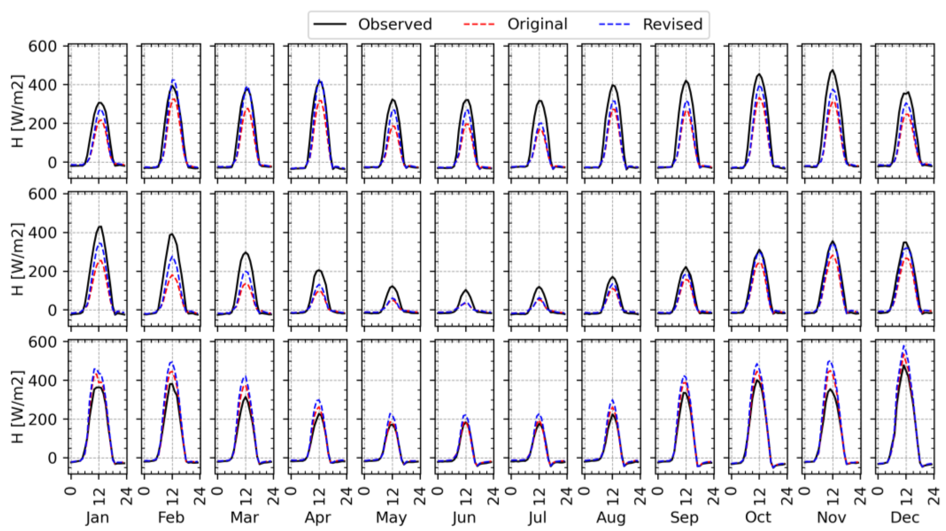
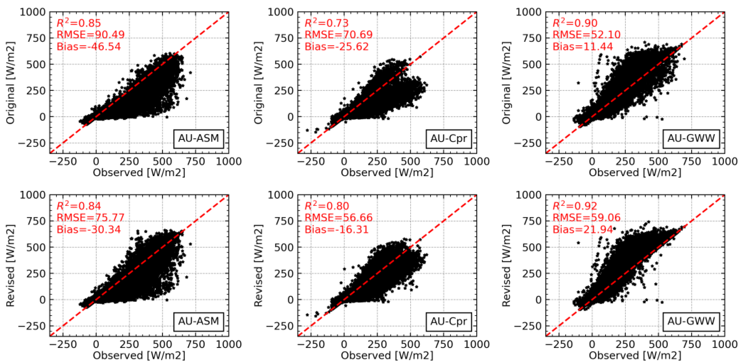
3.1. Savannah Sites
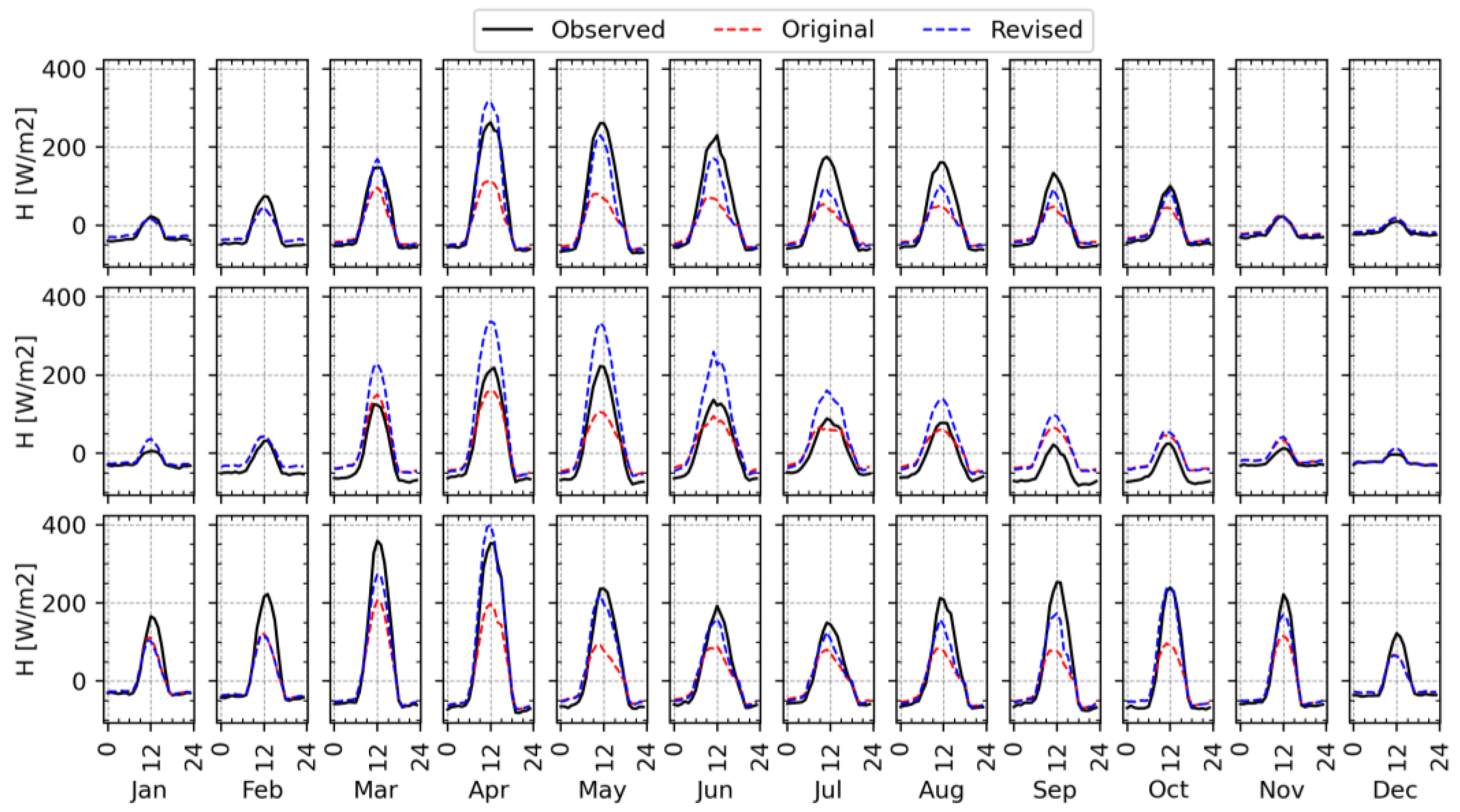
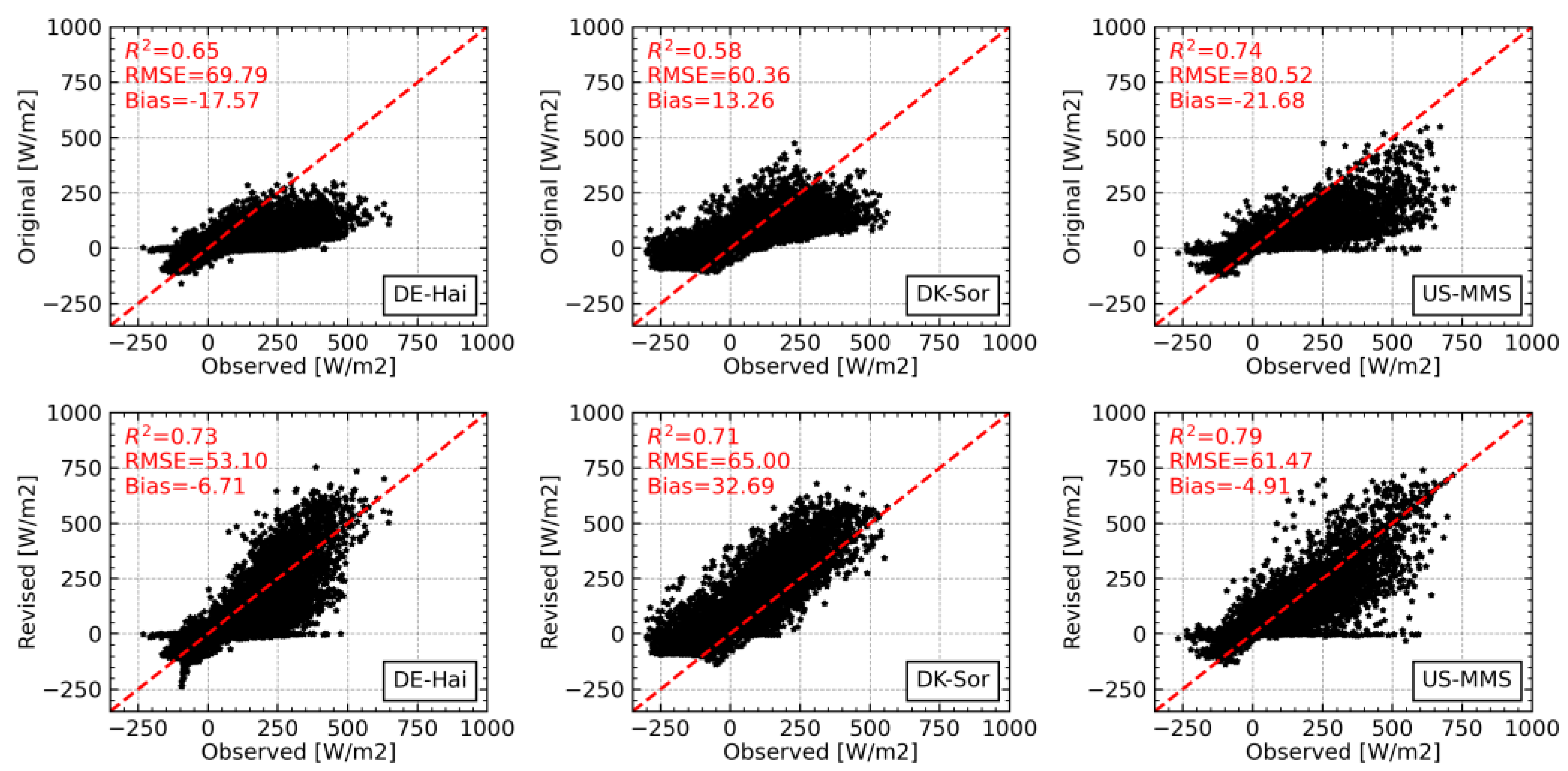
3.2. Deciduous Broad-Leaf Forest Sites
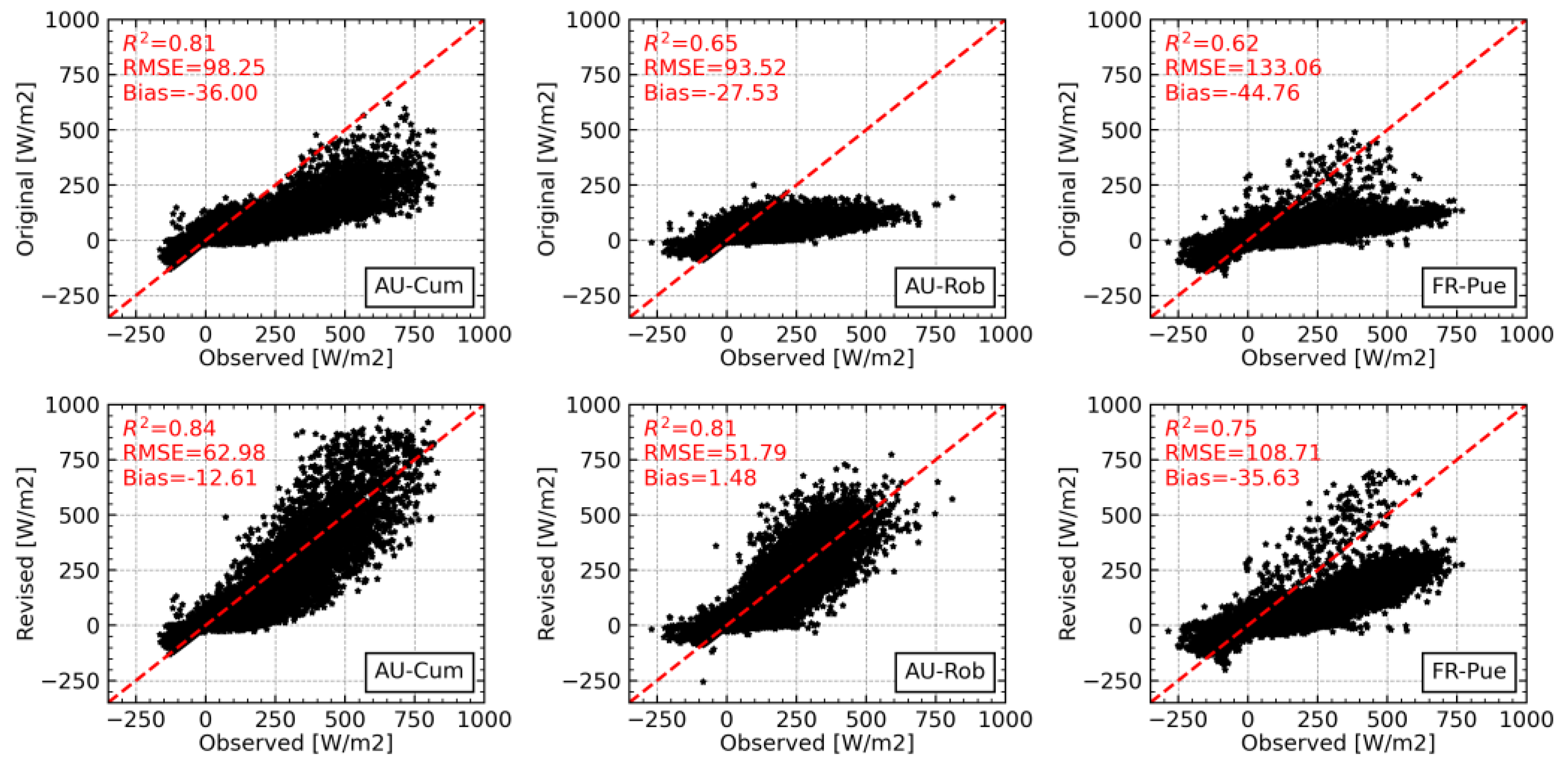
3.3. Evergreen Broad-Leaf Forest Sites
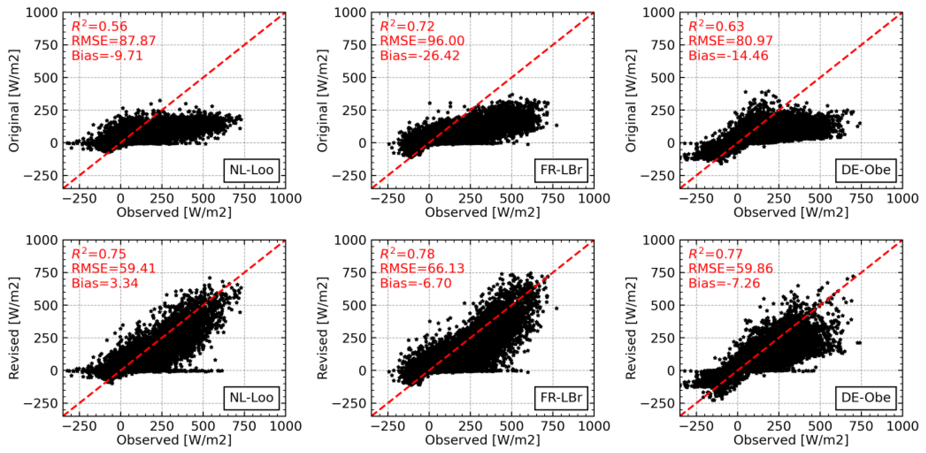
3.4. Evergreen Needle Leaf Forest Sites
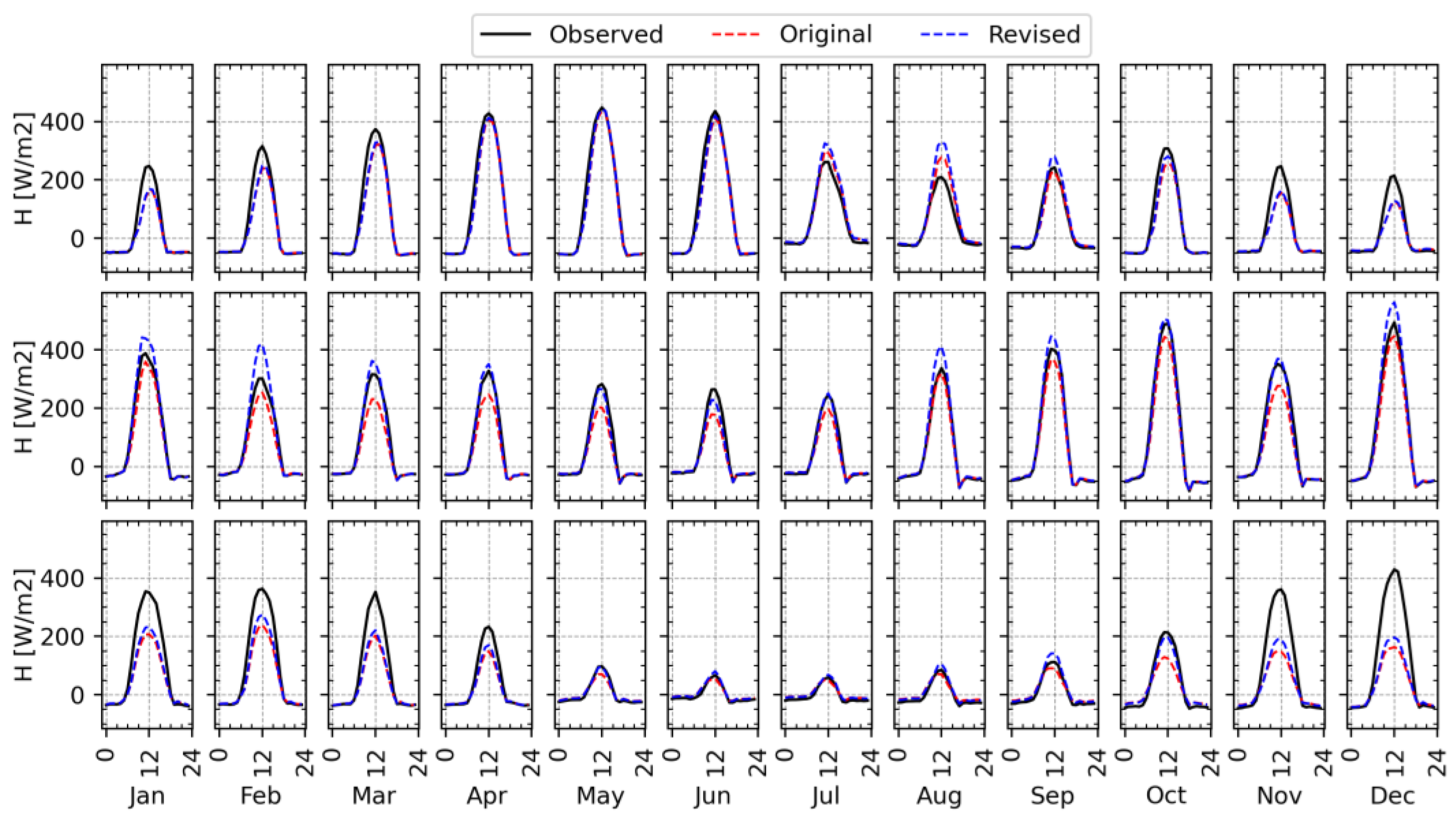
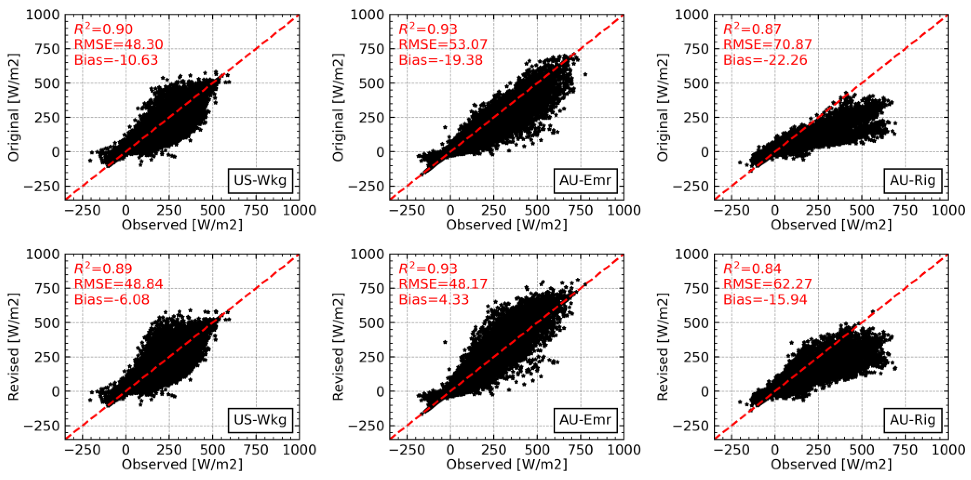
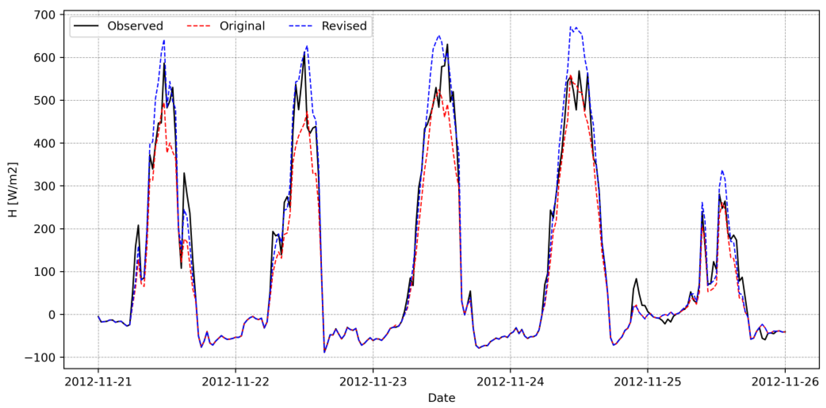
3.5. Grassland Sites
4. Discussion
5. Conclusions
Author Contributions
Funding
Data Availability Statement
Conflicts of Interest
References
- Su, Z. The Surface Energy Balance System (SEBS) for estimation of turbulent heat fluxes. Hydrol. Earth Syst. Sci. 2002, 6, 85–100. [Google Scholar] [CrossRef]
- Bastiaanssen, W.G.M.; Menenti, M.; Feddes, R.A.; Holtslag, A.A.M. A remote sensing surface energy balance algorithm for land (SEBAL). 1. Formulation. J. Hydrol. 1998, 212–213, 198–212. [Google Scholar] [CrossRef]
- Allen, R.G.; Tasumi, M.; Trezza, R. Satellite-Based Energy Balance for Mapping Evapotranspiration with Internalized Calibration (METRIC)—Model. J. Irrig. Drain. Eng. 2007, 133, 380–394. [Google Scholar] [CrossRef]
- Kustas, W.P.; Norman, J.M. A two-source approach for estimating turbulent fluxes using multiple angle thermal infrared observations. Water Resour. Res. 1997, 33, 1495–1508. [Google Scholar] [CrossRef]
- Norman, J.M.; Kustas, W.P.; Humes, K.S. Source approach for estimating soil and vegetation energy fluxes in observations of directional radiometric surface temperature. Agric. For. Meteorol. 1995, 77, 263–293. [Google Scholar] [CrossRef]
- Kalma, J.D.; McVicar, T.R.; McCabe, M.F. Estimating Land Surface Evaporation: A Review of Methods Using Remotely Sensed Surface Temperature Data. Surv. Geophys. 2008, 29, 421–469. [Google Scholar] [CrossRef]
- Timmermans, W.J.; Kwast, J.V.D.; Gieske, A.S.M.; Su, Z.; Olioso, A.; Jia, L.; Elbers, J. Intercomparison of Energy Flux Models Using ASTER Imagery at the Sparc 2004 SITE (BARRAX, SPAIN); Food and Agriculture Organization: Rome, Italy, 2004; pp. 1–8. [Google Scholar]
- Mallick, K.; Wandera, L.; Bhattarai, N.; Hostache, R.; Kleniewska, M.; Chormanski, J. A Critical Evaluation on the Role of Aerodynamic and Canopy–Surface Conductance Parameterization in SEB and SVAT Models for Simulating Evapotranspiration: A Case Study in the Upper Biebrza National Park Wetland in Poland. Water 2018, 10, 1753. [Google Scholar] [CrossRef] [Green Version]
- Owen, P.R.; Thomson, W.R. Heat transfer across rough surfaces. J. Fluid Mech. 1963, 15, 321–334. [Google Scholar] [CrossRef]
- Trebs, I.; Mallick, K.; Bhattarai, N.; Sulis, M.; Cleverly, J.; Woodgate, W.; Silberstein, R.; Hinko-Najera, N.; Beringer, J.; Meyer, W.S.; et al. The role of aerodynamic resistance in thermal remote sensing-based evapotranspiration models. Remote. Sens. Environ. 2021, 264, 112602. [Google Scholar] [CrossRef]
- Su, Z.; Schmugge, T.; Kustas, W.P.; Massman, W.J. An Evaluation of Two Models for Estimation of the Roughness Height for Heat Transfer between the Land Surface and the Atmosphere. J. Appl. Meteorol. 2001, 40, 1933–1951. [Google Scholar] [CrossRef]
- Kustas, W.; Choudhury, B.; Moran, M.; Reginato, R.; Jackson, R.; Gay, L.; Weaver, H. Determination of sensible heat flux over sparse canopy using thermal infrared data. Agric. For. Meteorol. 1989, 44, 197–216. [Google Scholar] [CrossRef]
- Blümel, K. A Simple Formula for Estimation of the Roughness Length for Heat Transfer over Partly Vegetated Surfaces. J. Appl. Meteorol. 1999, 38, 814–829. [Google Scholar] [CrossRef]
- Troufleau, D.; Lhomme, J.; Monteny, B.; Vidal, A. Sensible heat flux and radiometric surface temperature over sparse Sahelian vegetation. I. An experimental analysis of the kB−1 parameter. J. Hydrol. 1997, 188-189, 815–838. [Google Scholar] [CrossRef]
- Verhoef, A.; De Bruin, H.A.R.; Van Den Hurk, B.J.J.M. Some Practical Notes on the Parameter KB-1 for Sparse Vegetation. J. Appl. Meteorol. 1997, 36, 560–572. [Google Scholar] [CrossRef]
- van der Kwast, J.; Timmermans, W.; Gieske, A.; Su, Z.; Olioso, A.; Jia, L.; Elbers, J.; Karssenberg, D.; de Jong, S. Evaluation of the Surface Energy Balance System (SEBS) Applied to ASTER Imagery with Flux-Measurements at the SPARC 2004 Site (Barrax, Spain). Hydrol. Earth Syst. Sci. 2009, 13, 1337–1347. [Google Scholar] [CrossRef] [Green Version]
- Gokmen, M.; Vekerdy, Z.; Lubczynski, M.W.; Timmermans, J.; Batelaan, O.; Verhoef, W. Assessing Groundwater Storage Changes Using Remote Sensing–Based Evapotranspiration and Precipitation at a Large Semiarid Basin Scale. J. Hydrometeorol. 2013, 14, 1733–1753. [Google Scholar] [CrossRef]
- Huang, C.; Li, Y.; Gu, J.; Lu, L.; Li, X. Improving Estimation of Evapotranspiration under Water-Limited Conditions Based on SEBS and MODIS Data in Arid Regions. Remote Sens. 2015, 7, 16795–16814. [Google Scholar] [CrossRef] [Green Version]
- Chen, X.; Massman, W.J.; Su, Z. A Column Canopy-Air Turbulent Diffusion Method for Different Canopy Structures. J. Geophys. Res. Atmos. 2019, 124, 488–506. [Google Scholar] [CrossRef]
- Gokmen, M.; Vekerdy, Z.; Verhoef, A.; Verhoef, W.; Batelaan, O.; van der Tol, C. Integration of Soil Moisture in SEBS for Improving Evapotranspiration Estimation under Water Stress Conditions. Remote Sens. Environ. 2012, 121, 261–274. [Google Scholar] [CrossRef]
- Chen, X.; Su, Z.; Ma, Y.; Yang, K.; Wen, J.; Zhang, Y. An Improvement of Roughness Height Parameterization of the Surface Energy Balance System (SEBS) over the Tibetan Plateau. J. Appl. Meteorol. Climatol. 2013, 52, 607–622. [Google Scholar] [CrossRef] [Green Version]
- Brutsaert, W. Heat and Mass Transfer to and from Surfaces with Dense Vegetation or Similar Permeable Roughness. Boundary-Layer Meteorol. 1979, 16, 365–388. [Google Scholar] [CrossRef]
- Ukkola, A. PLUMBER2: Forcing and Evaluation Datasets for a Model Intercomparison Project for Land Surface Models, Version 1.0; NCI National Research Data Collection: Canberra, Australia, 2020. [CrossRef]
- Ukkola, A.M.; Abramowitz, G.; De Kauwe, M.G. A Flux Tower Dataset Tailored for Land Model Evaluation. Earth Syst. Sci. Data 2022, 14, 449–461. [Google Scholar] [CrossRef]
- Pastorello, G.; Trotta, C.; Canfora, E.; Chu, H.; Christianson, D.; Cheah, Y.W.; Poindexter, C.; Chen, J.; Elbashandy, A.; Humphrey, M.; et al. The FLUXNET2015 Dataset and the ONEFlux Processing Pipeline for Eddy Covariance Data. Sci. Data 2020, 7, 225. [Google Scholar] [CrossRef] [PubMed]
- Isaac, P.; Cleverly, J.; McHugh, I.; Van Gorsel, E.; Ewenz, C.; Beringer, J. OzFlux Data: Network Integration from Collection to Curation. Biogeosciences 2017, 14, 2903–2928. [Google Scholar] [CrossRef] [Green Version]
- Sobrino, J.A.; Jiménez-Muñoz, J.C.; Paolini, L. Land Surface Temperature Retrieval from LANDSAT TM 5. Remote Sens. Environ. 2004, 90, 434–440. [Google Scholar] [CrossRef]
- Castellví, F.; Snyder, R.L.; Baldocchi, D.D. Surface Energy-Balance Closure over Rangeland Grass Using the Eddy Covariance Method and Surface Renewal Analysis. Agric. For. Meteorol. 2008, 148, 1147–1160. [Google Scholar] [CrossRef]
- Arnqvist, J.; Bergström, H. Flux-Profile Relation with Roughness Sublayer Correction. Q. J. R. Meteorol. Soc. 2015, 141, 1191–1197. [Google Scholar] [CrossRef]
- Garratt, J.R. Surface Influence upon Vertical Profiles in the Atmospheric Near-surface Layer. Q. J. R. Meteorol. Soc. 1980, 106, 803–819. [Google Scholar] [CrossRef]
- Choudhury, B.J.; Monteith, J.L. A Four-Layer Model for the Heat Budget of Homogeneous Land Surfaces. Q. J. R. Meteorol. Soc. 1988, 114, 373–398. [Google Scholar] [CrossRef]
- Brutsaert, W. Evaporation into the Atmosphere; Springer: Dordrecht, The Netherlands, 1982. [Google Scholar]
- Wang, W.J.; Peng, W.Q.; Huai, W.X.; Katul, G.G.; Liu, X.B.; Qu, X.D.; Dong, F. Friction Factor for Turbulent Open Channel Flow Covered by Vegetation. Sci. Rep. 2019, 9, 5178. [Google Scholar] [CrossRef] [Green Version]


| Variable | Meteorological | Remote Sensing |
|---|---|---|
| Land surface temperature (LST) | yes | |
| Leaf Area Index (LAI) | yes | |
| Fraction vegetation cover | yes | |
| Land Surface albedo | yes | |
| Land surface emissivity | yes | |
| Vegetation roughness/Canopy height | yes | |
| Down-welling solar radiation | yes | yes |
| Down-welling longwave radiation | yes | yes |
| Air temperature | yes | |
| Air pressure | yes | |
| Humidity | yes | |
| Wind speed | yes |
| Country | Location | Station Code | Longitude | Latitude | Vegetation | Canopy Height [m] | Study Period |
|---|---|---|---|---|---|---|---|
| Germany | Hainich | DE-Hai | 10.4522 | 51.0792 | DBF | 33.0 | [2007, 2008] |
| Denmark | Soroe | DK-Sor | 11.6446 | 55.4859 | DBF | 25.0 | [2011, 2012] |
| USA | Morgan Monroe State Forest | US-MMS | −86.4131 | 39.3232 | DBF | 27.0 | [2009, 2010] |
| Australia | Cumberland Plains | AU-Cum | 150.7236 | −33.6152 | EBF | 23.0 | [2016, 2017] |
| Australia | Robson Creek | AU-Rob | 145.6301 | −17.1175 | EBF | 44.0 | [2015, 2016] |
| France | Puechabon | FR-Pue | 3.5957 | 43.7413 | EBF | 6.5 | [2010, 2011] |
| Netherlands | Loobos | NL-Loo | 5.7436 | 52.1666 | ENF | 15.5 | [2009, 2010] |
| France | Le Bray | FR-LBr | −0.7693 | 44.7171 | ENF | 20.0 | [2005, 2006] |
| Germany | Oberbärenburg | DE-Obe | 13.7213 | 50.7867 | ENF | 19.0 | [2012, 2013] |
| USA | Walnut Gulch Kendall Grasslands | US-Wkg | −109.9419 | 31.7365 | Grassland | 1.0 | [2011, 2012] |
| Australia | Emerald | AU-Emr | 148.4746 | −23.8587 | Grassland | 2.0 | [2012, 2013] |
| Australia | Riggs Creek | AU-Rig | 145.5759 | −36.6499 | Grassland | 0.4 | [2015, 2016] |
| Australia | Alice Springs | AU-ASM | 133.2490 | −22.2830 | Savannah | 6.5 | [2016, 2017] |
| Australia | Calperum | AU-Cpr | 140.5891 | −34.0021 | Savannah | 4.0 | [2013, 2014] |
| Australia | Great Western Woodlands | AU-GWW | 120.6541 | −30.1913 | Savannah | 18.0 | [2014, 2015] |
Disclaimer/Publisher’s Note: The statements, opinions and data contained in all publications are solely those of the individual author(s) and contributor(s) and not of MDPI and/or the editor(s). MDPI and/or the editor(s) disclaim responsibility for any injury to people or property resulting from any ideas, methods, instructions or products referred to in the content. |
© 2023 by the authors. Licensee MDPI, Basel, Switzerland. This article is an open access article distributed under the terms and conditions of the Creative Commons Attribution (CC BY) license (https://creativecommons.org/licenses/by/4.0/).
Share and Cite
Njuki, S.M.; Mannaerts, C.M.; Su, Z. Accounting for Turbulence-Induced Canopy Heat Transfer in the Simulation of Sensible Heat Flux in SEBS Model. Remote Sens. 2023, 15, 1578. https://doi.org/10.3390/rs15061578
Njuki SM, Mannaerts CM, Su Z. Accounting for Turbulence-Induced Canopy Heat Transfer in the Simulation of Sensible Heat Flux in SEBS Model. Remote Sensing. 2023; 15(6):1578. https://doi.org/10.3390/rs15061578
Chicago/Turabian StyleNjuki, Sammy M., Chris M. Mannaerts, and Zhongbo Su. 2023. "Accounting for Turbulence-Induced Canopy Heat Transfer in the Simulation of Sensible Heat Flux in SEBS Model" Remote Sensing 15, no. 6: 1578. https://doi.org/10.3390/rs15061578