

Application of a Fusion Model Based on Machine Learning in Visibility Prediction
 , , and
Abstract
:
1. Introduction
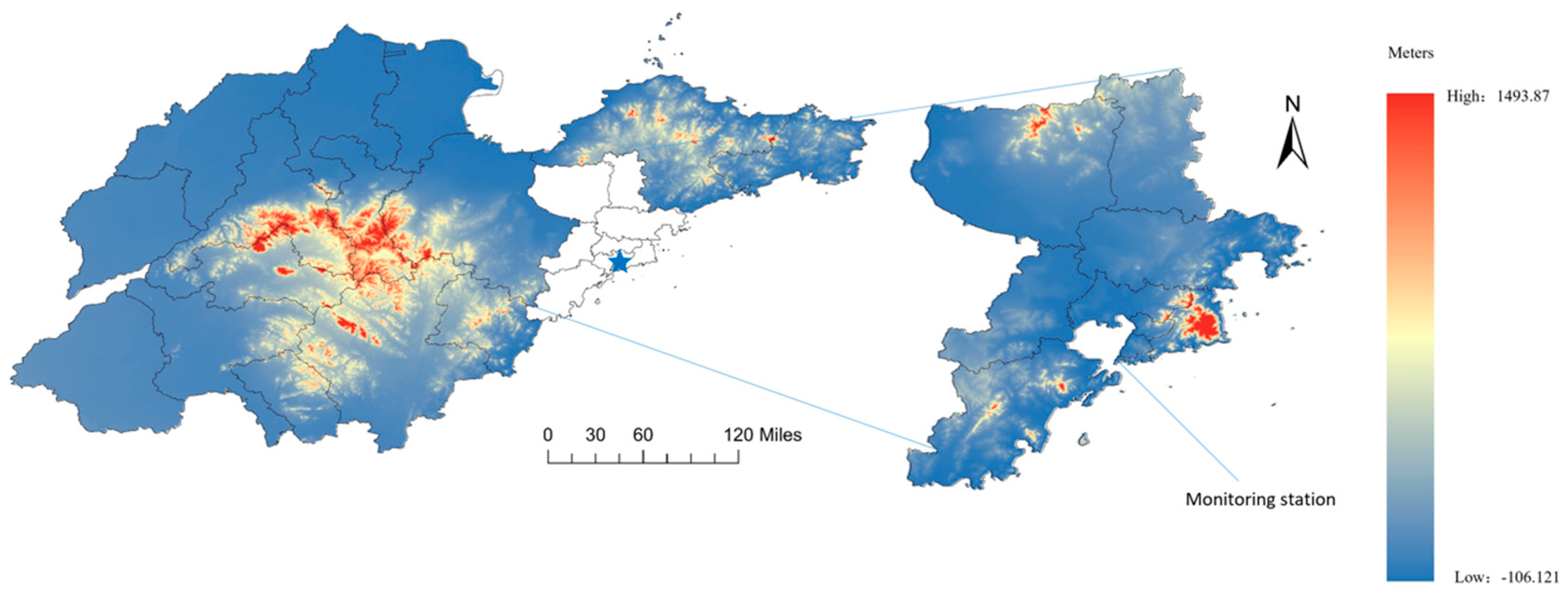
2. Data Source
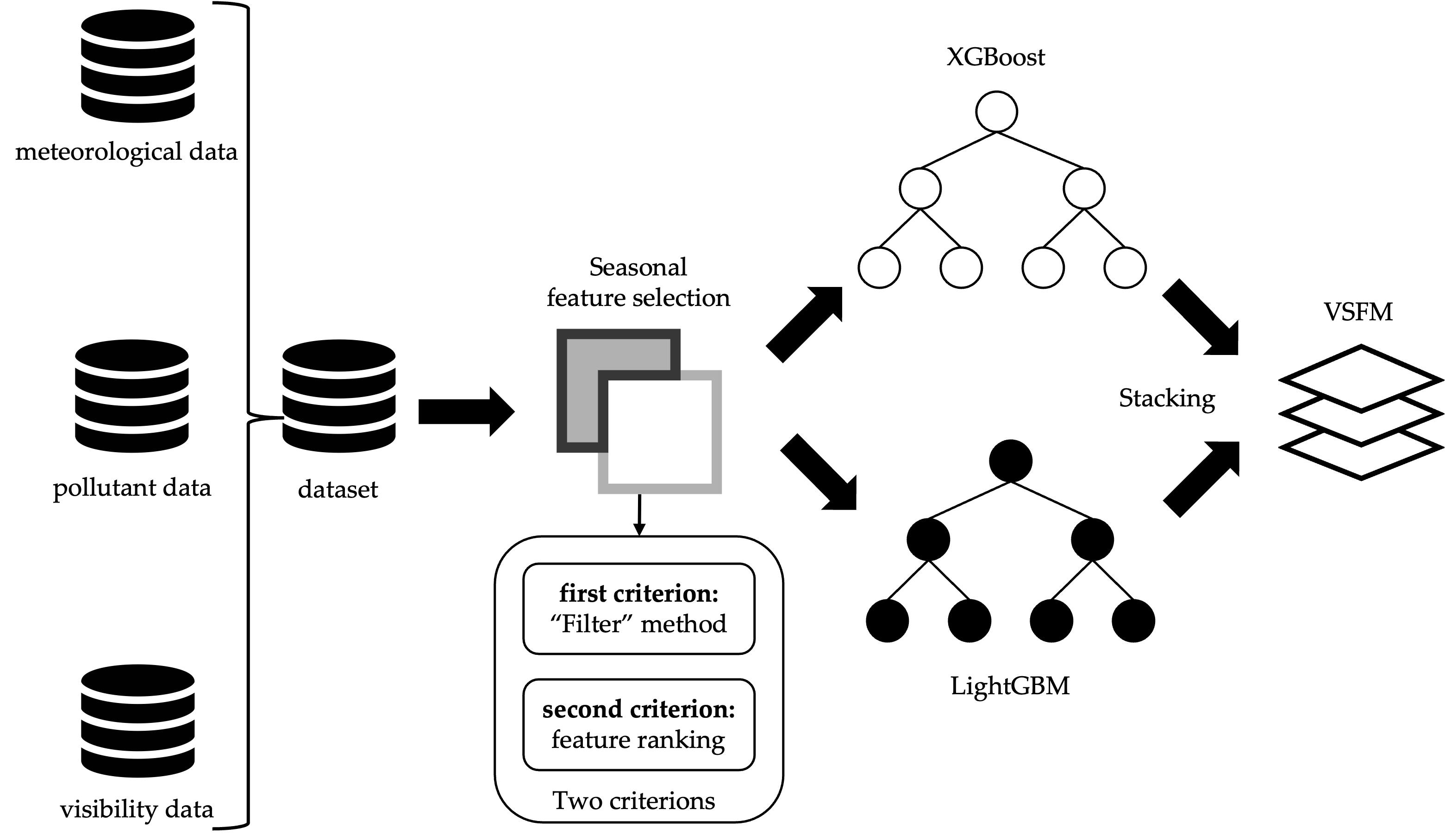
3. Method
3.1. Construction of the Fusion Model
3.1.1. XGBoost
- Regularization processing—XGBoost introduces regular terms to control the complexity of the tree in order to avoid overfitting and make the trained model simpler. In this way, its generalization performance is higher than that of GBDT.
- Loss function optimization—second-order Taylor expansion is performed on the loss function, and the first-order derivative and second-order derivative information is used to determine the output result, which speeds up the training.
- Strong flexibility—in addition to CART as a base learner, XGBoost also supports linear classifiers. Furthermore, XGBoost can customize the evaluation function, which is conducive to evaluating results from multiple performance metrics.
- Improvement in the node division method—when seeking the optimal splitting point, XGBoost abandons traditional greedy algorithm segmentation and adopts the approximate greedy strategy algorithm to accelerate the leaf node splitting process and reduce the consumption of computing resources.
3.1.2. LightGBM
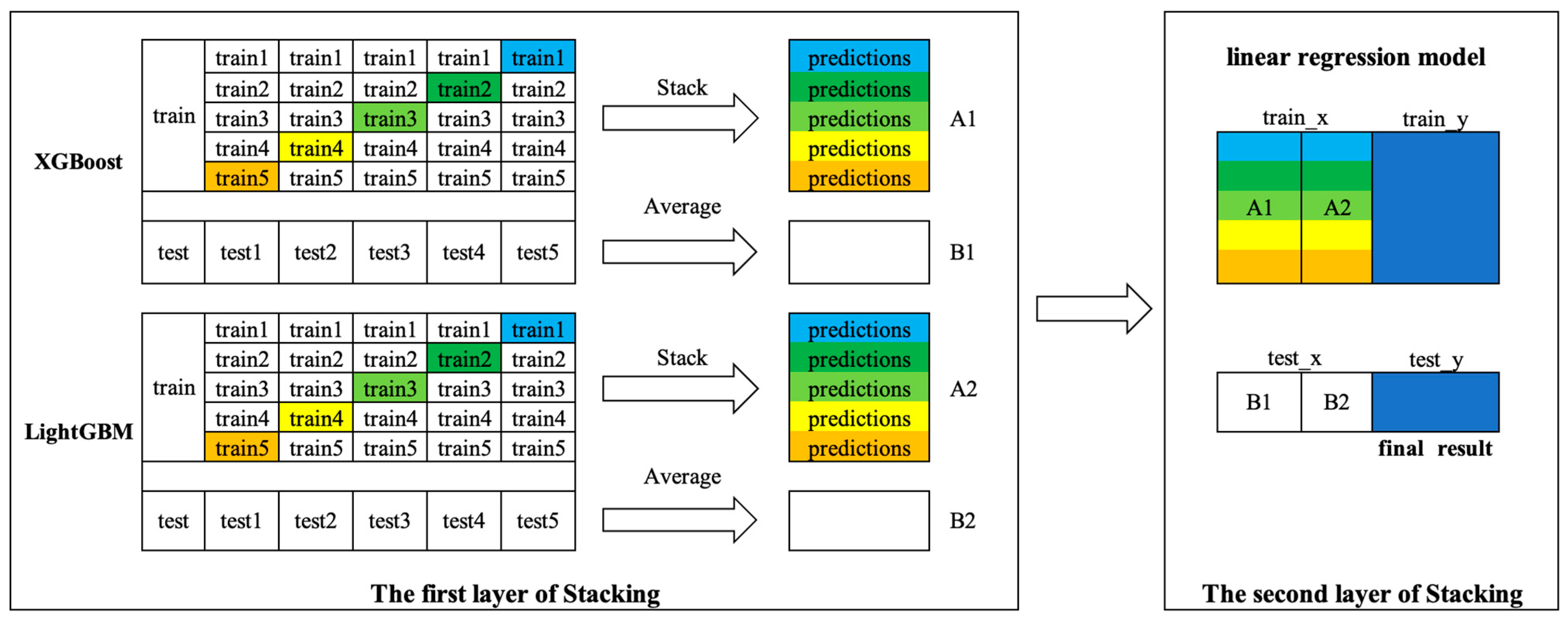
3.1.3. Stacking Fusion Model
- Data set generation—firstly, the strategy generates a training set and a test set and divides the training set into five parts: train1, train2, train3, train4, and train5.
- Base learner training—for each base learner (the first layer of stacking), train1, train2, train3, train4, and train5 are used in turn as the validation set, and the remaining four parts are used as the training set. Five-fold cross-validation is performed for model training and validation, and five copies of the validation (“predictions”) are obtained. Then, predictions are made on the test set to obtain five predicted values.
- Fusion model training—in this paper, a linear regression (LR) model was chosen as the fusion model (the second layer of stacking). The validations of the two base models are vertically overlapped (A1 and A2) as the train_x of the LR model and the corresponding true values are used as train_y of the LR model.
- Fusion model prediction—the prediction values on the five test sets of base learners are averaged (B1 and B2) as the test_x of the LR model; then, using the trained LR model in Step 3 and test_x to make predictions, test_y is obtained as the final prediction result.
3.2. Feature Engineering
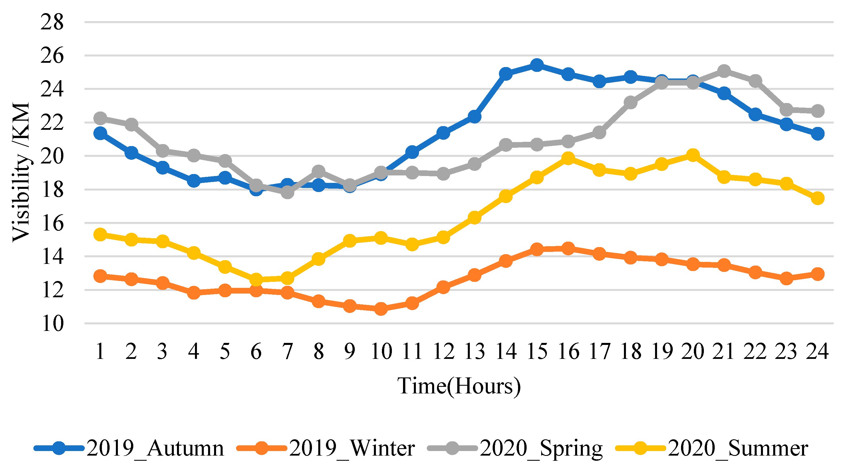
3.2.1. Seasonal Characteristics of Visibility in Qingdao
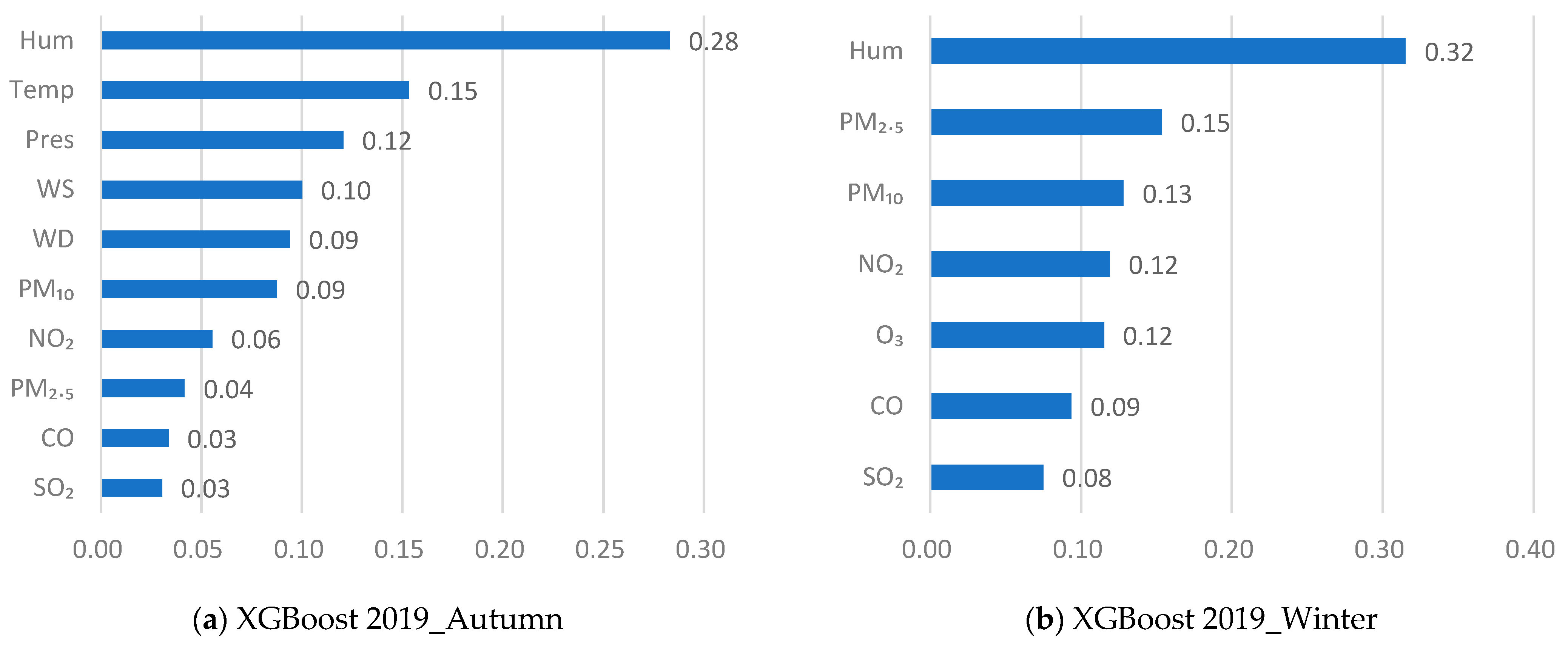
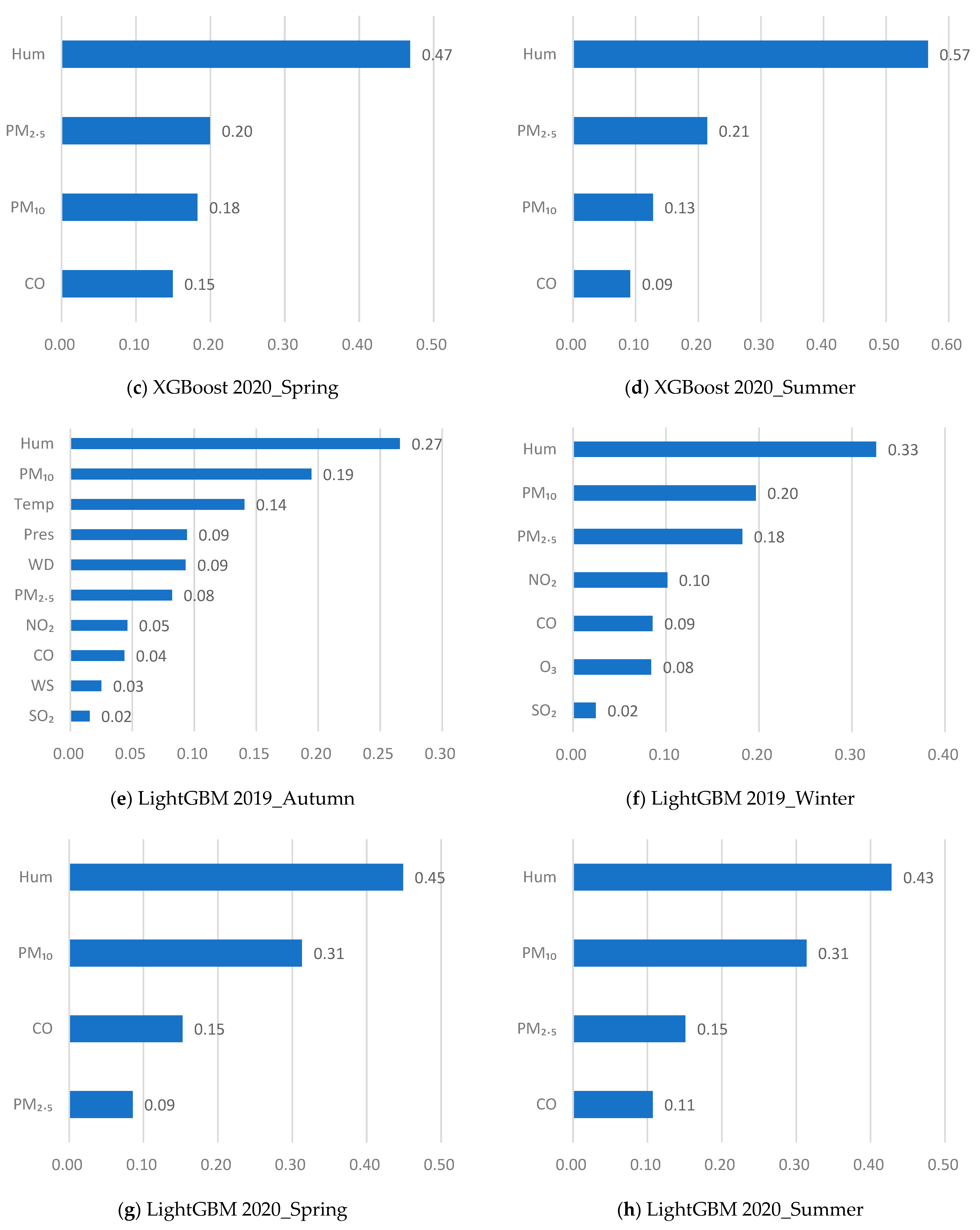
3.2.2. Seasonal Feature Selection
3.3. Performance Metrics
4. Results
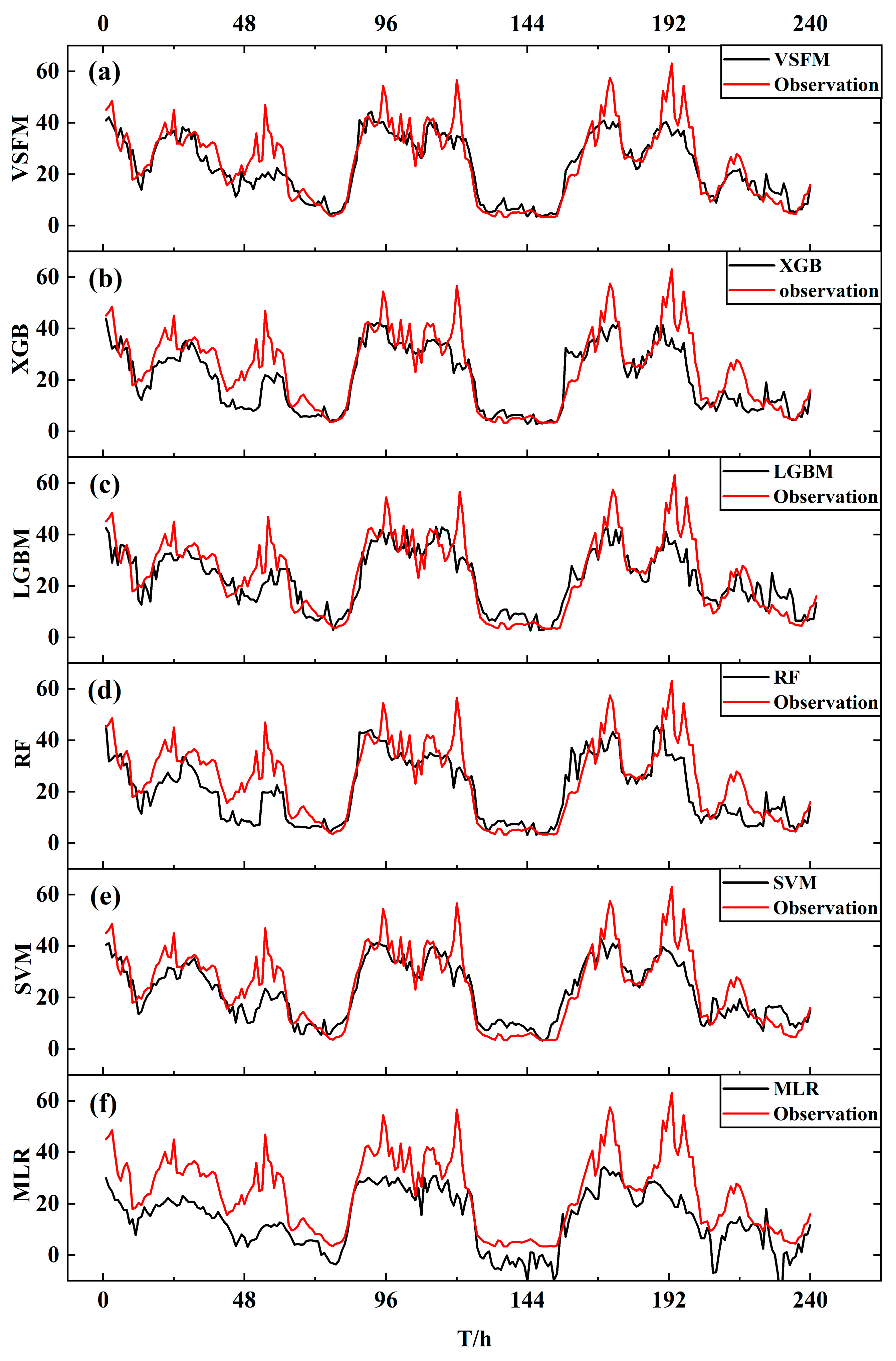
4.1. Comparison and Analysis of the Performance Metrics of Each Model
4.2. Visibility Classification Performance
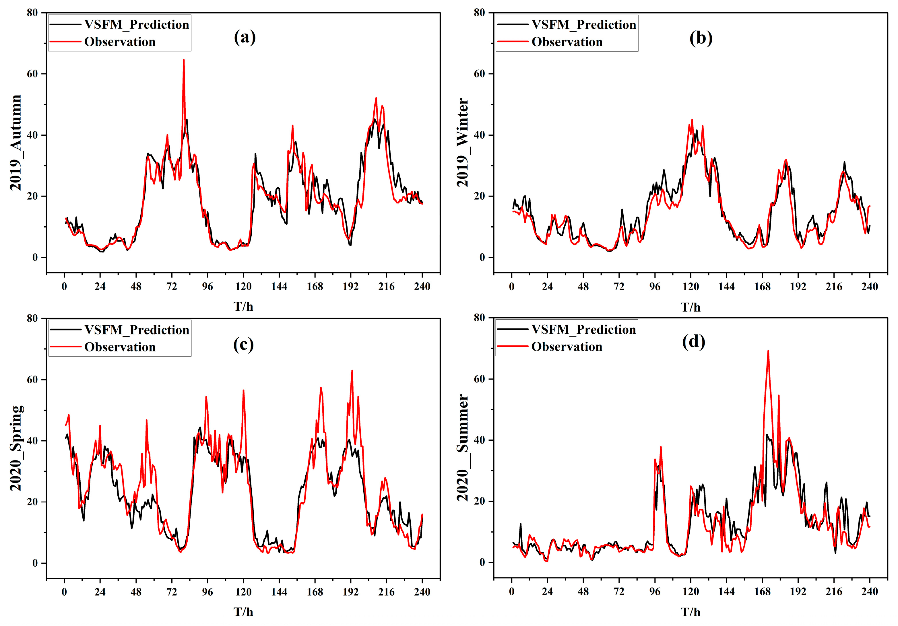
4.3. Prediction Effect of the VSFM in Each Season
5. Discussion
6. Conclusions
- The range of seasonal visibility changes in Qingdao and possible causes were analyzed in relation to meteorological and pollutant parameters. It was evident that there were seasonal differences in pollution sources and affecting factors in northern cities of China. Visibility was mainly affected by heating in the winter. In the summer, high humidity and frequent sea fog had a major impact on visibility. In the autumn, visibility was mainly affected by transported pollutants. Visibility was quite good in the spring due to the rather dry and clean air. The seasonal differences in pollution sources and factors affecting visibility support the need for seasonal feature selection and visibility prediction in Qingdao.
- Based on the seasonal characteristics of visibility in Qingdao, seasonal feature selection for visibility prediction was designed and implemented. Feature importance criteria based on the “Filter” method and feature ranking were constructed for seasonal feature selection, and different feature factors were found that strongly correlated with the different pollution sources in different seasons. Evaluation results showed that applying feature selection reduced the RMSE by 0.9834 km and the MAE by 0.7459 km, and increased the CC by 2.99%;
- Performance metrics of the VSFM, such as the RMSE, MAE, and CC, were evaluated. The results showed that the VSFM could effectively improve the accuracy of visibility prediction when the basic learners performed well. The VSFM reduced the RMSE by 0.0089–1.3795 km and MAE by 0.2819–1.7646 km, and improved the CC by 0.91–4.28% and the TS score by 0.0269–0.4573 when compared to XGBoost and LightGBM;
- The TS scores of the VSFM and other single models were compared. The results showed that the VSFM significantly improved prediction accuracy under different classifications of visibility. Its advantage was especially obvious in extremely low visibility (V < 2 km, Class I). Under class I conditions, the VSFM had a TS score of 0.5, while the other models had scores less than ~0.27.
Author Contributions
Funding
Data Availability Statement
Acknowledgments
Conflicts of Interest
References
- Horvath, H. Atmospheric visibility. Atmos. Environ. 1981, 15, 1785–1796. [Google Scholar] [CrossRef]
- Deng, X.; Tie, X.; Wu, D.; Zhou, X.; Bi, X.; Tan, H.; Li, F.; Jiang, C. Long-term trend of visibility and its characterizations in the Pearl River Delta (PRD) region, China. Atmos. Environ. 2008, 42, 1424–1435. [Google Scholar] [CrossRef]
- Qian, W.; Leung, J.C.-H.; Chen, Y.; Huang, S. Applying anomaly-based weather analysis to the prediction of low visibility associated with the coastal fog at Ningbo-Zhoushan Port in East China. Adv. Atmos. Sci. 2019, 36, 1060–1077. [Google Scholar] [CrossRef] [Green Version]
- Gultepe, I.; Sharman, R.; Williams, P.D.; Zhou, B.; Ellrod, G.; Minnis, P.; Trier, S.; Griffin, S.; Yum, S.S.; Gharabaghi, B.; et al. A review of high impact weather for aviation meteorology. Pure Appl. Geo-Phys. 2019, 176, 1869–1921. [Google Scholar] [CrossRef]
- Chen, R.; Wang, X.; Meng, X.; Hua, J.; Zhou, Z.; Chen, B.; Kan, H. Communicating air pollution-related health risks to the public: An application of the Air Quality Health Index in Shanghai, China. Environ. Int. 2013, 51, 168–173. [Google Scholar] [CrossRef]
- Jacobson, M.Z. Comment on “fully coupled ‘online’ chemistry within the WRF model”, by Grell et al., 2005. Atmospheric Environment 39, 6957–6975. Atmos. Environ. 2006, 40, 4646–4648. [Google Scholar] [CrossRef]
- Binkowski, F.S.; Roselle, S.J. Models-3 community multiscale air quality (cmaq) model aerosol component 1. model description. J. Geophys. Res. Atmos. 2003, 108, 4183. [Google Scholar] [CrossRef]
- Cheng, F.; Feng, C.; Yang, Z.; Hsu, C.; Chan, K.; Lee, C.; Chang, S. Evaluation of real-time PM2.5 forecasts with the WRF-CMAQ modeling system and weather-pattern-dependent bias-adjusted PM2.5 forecasts in Taiwan. Atmos. Environ. 2020, 244, 117909. [Google Scholar] [CrossRef]
- Grell, G.A.; Peckham, S.E.; Schmitz, R.; McKeen, S.A.; Frost, G.; Skamarock, W.C.; Eder, B. Fully coupled "online" chemistry within the WRF model. Atmos. Environ. 2005, 39, 6957–6975. [Google Scholar] [CrossRef]
- Zhou, G.; Xu, J.; Xie, Y.; Chang, L.; Gao, W.; Gu, Y.; Zhou, J. Numerical air quality forecasting over eastern China: An operational application of WRF-Chem—ScienceDirect. Atmos. Environ. 2017, 153, 94–108. [Google Scholar] [CrossRef]
- An, X.Q.; Zhai, S.X.; Jin, M.; Gong, S.; Wang, Y. Development of an adjoint model of GRAPES–CUACE and its application in tracking influential haze source areas in north China. Geosci. Model Dev. 2016, 9, 2153–2165. [Google Scholar] [CrossRef]
- Yang, D.; Ritchie, H.; Desjardins, S.; Pearson, G.; MacAfee, A.; Gultepe, I. High-Resolution GEM-LAM Application in Marine Fog Prediction: Evaluation and Diagnosis. Weather Forecast. 2009, 25, 727–748. [Google Scholar] [CrossRef]
- Shi, H. Analysis of Factors Affecting Visibility and Its Variation Features in Pudong Area of Shanghai. Atmos. Sci. Res. Appl. 2008, 02, 1–8. [Google Scholar]
- Liang, X.; Zhou, T.; Guo, B.; Li, S.; Zhang, H.; Zhang, S.; Huang, H.; Chen, S.X. Assessing Beijing’s PM2.5 pollution: Severity, weather impact, APEC and winter heating. Proc. R. Soc. A 2015, 471, 20150257. [Google Scholar] [CrossRef] [Green Version]
- Tang, H.; Wei, Z.; Liu, J. Visibility Prediction Based On XGBoost And Markov Chain Combined Model. In Proceedings of the 7th International Conference on Computer and Communications (ICCC), Wuhan, China, 22—25 April 2022; pp. 1617–1622. [Google Scholar]
- Yu, D.; Zhao, W.; Nie, K.; Zhang, G. Visibility forecast model based on LightGBM algorithm. J. Comput. Appl. 2021, 41, 1035–1041. [Google Scholar]
- Kim, B.Y.; Cha, J.W.; Chang, K.H.; Lee, C. Visibility Prediction over South Korea Based on Random Forest. Atmos. 2021, 12, 552. [Google Scholar] [CrossRef]
- Lo, W.L.; Zhu, M.; Fu, H. Meteorology visibility estimation by using multi-support vector regression method. J. Adv. Inf. Technol. 2020, 11, 40–47. [Google Scholar] [CrossRef]
- Chevalier, R.F.; Hoogenboom, G.; Mcclendon, R.W.; Paz, J.A. Support vector regression with reduced training sets for air temperature prediction: A comparison with artificial neural networks. Neural Comput. Appl. 2011, 20, 151–159. [Google Scholar] [CrossRef]
- Bari, D. Visibility Prediction Based on Kilometric NWP Model Outputs Using Machine-Learning Regression. In Proceedings of the 14th International Conference on e-Science (e-Science), Amsterdam, Netherlands, 29 October—1 November 2018; p. 278. [Google Scholar]
- Guijo-Rubio, D.; Gutiérrez, P.A.; Casanova-Mateo, C.; Sanz-Justo, J.; Salcedo-Sanz, S.; Hervás-Martínez, C. Prediction of low-visibility events due to fog using ordinal classification. Atmos. Res. 2018, 214, 64–73. [Google Scholar] [CrossRef]
- Kneringer, P.; Dietz, S.J.; Mayr, G.J.; Zeileis, A. Probabilistic nowcasting of low-visibility procedure states at Vienna International Airport during cold season. Pure Appl. Geo-Phys. 2019, 176, 2165–2177. [Google Scholar] [CrossRef] [Green Version]
- Zhu, L.; Zhu, G.; Han, L.; Wang, N. The application of deep learning in airport visibility forecast. Atmos. Clim. Sci. 2017, 7, 314. [Google Scholar] [CrossRef] [Green Version]
- Yu, X.; Ma, J.; An, J.; Yuan, L.; Zhu, B.; Liu, D.; Wang, J.; Yang, Y.; Cui, H. Impacts of meteorological condition and aerosol chemical compositions on visibility impairment in Nanjing, China. J. Clean Prod. 2016, 131, 112–120. [Google Scholar] [CrossRef]
- Xiao, Q.; Chang, H.H.; Geng, G.; Liu, Y. An ensemble machine-learning model to predict historical PM2.5 concentrations in China from satellite data. Environ. Sci. Technol. 2018, 52, 13260–13269. [Google Scholar] [CrossRef]
- Xu, Y.; Ho, H.C.; Wong, M.S.; Deng, C.; Shi, Y.; Chan, T.C.; Knudby, A. Evaluation of machine learning techniques with multiple remote sensing datasets in estimating monthly concentrations of ground-level PM2.5. Environ. Pollut. 2018, 242, 1417–1426. [Google Scholar] [CrossRef]
- Zhang, C.; Wu, M.; Chen, J.; Chen, K.; Zhang, C.; Xie, C.; Huang, B.; He, Z.C. Weather Visibility Prediction Based on Multimodal Fusion. IEEE Access 2019, 7, 74776–74786. [Google Scholar] [CrossRef]
- Friedman, J.H. Greedy function approximation: A gradient boosting machine. Ann. Stat. 2001, 29, 1189–1232. [Google Scholar] [CrossRef]
- Chen, T.; He, T.; Benesty, M.; Khotilovich, V.; Tang, Y.; Cho, H.; Chen, K. XGBoost: Extreme Gradient Boosting; R Package Version 0.4-2; R Core Team: Vienna, Austria, 2015; Volume 1; pp. 1–4. [Google Scholar]
- Ke, G.; Meng, Q.; Finley, T.; Wang, T.; Chen, W.; Ma, W.; Ye, Q.; Liu, T.Y. Lightgbm: A highly efficient gradient boosting decision tree. In Proceedings of the 31st Conference on Neural Information Processing Systems (NIPS 2017), Long Beach, CA, USA, 8–9 December 2017; p. 30. [Google Scholar]
- Ma, J.; Yu, Z.; Qu, Y.; Xu, J.; Cao, Y. Application of the XGBoost Machine Learning Method in PM2.5 Prediction: A Case Study of Shanghai. Aerosol Air Qual. Res. 2020, 20, 128–138. [Google Scholar] [CrossRef] [Green Version]
- Zhai, B.; Chen, J. Development of a stacked ensemble model for forecasting and analyzing daily average PM2.5 concentrations in Beijing, China. Sci. Total Environ. 2018, 635, 644–658. [Google Scholar] [CrossRef]
- Zhong, J.; Zhang, X.; Gui, K.; Wang, Y.; Che, H.; Shen, X.; Zhang, L.; Zhang, Y.; Sun, J.; Zhang, W. Robust prediction of hourly PM2.5 from meteorological data using Light GBM. Natl. Sci. Rev. 2021, 8, nwaa307. [Google Scholar] [CrossRef] [PubMed]
- Polikar, R. Essemble based systems in decision making. IEEE Circ. Syst. Mag. 2006, 6, 21–45. [Google Scholar] [CrossRef]
- Sheng, L.; Liang, W.; Wang, D.; Gao, S. Analysis of the influence of changes in marine meteorological conditions on the advection fog process in Qingdao. Period. Ocean Univ. China 2010, 40, 1–10. [Google Scholar]


| Type | Parameter | Abbreviation | Unit | Description |
|---|---|---|---|---|
| Meteorological factors | Temperature | Temp | °C | Hourly average air temperature |
| Humidity | Hum | % | Hourly average relative humidity | |
| Pressure | Pres | hPa | Hourly average barometric pressure | |
| Wind speed | WS | m/s | Hourly average wind speed | |
| Wind direction | WD | deg | Hourly average wind direction | |
| Pollutant factors | PM2.5 | PM2.5 | μg·m−3 | Hourly average concentration of PM2.5 |
| PM10 | PM10 | μg·m−3 | Hourly average concentration of PM10 | |
| NO2 | NO2 | μg·m−3 | Hourly average concentration of NO2 | |
| O3 | O3 | μg·m−3 | Hourly average concentration of O3 | |
| SO2 | SO2 | μg·m−3 | Hourly average concentration of SO2 | |
| CO | CO | μg·m−3 | Hourly average concentration of CO | |
| Visibility | Visibility | V | km | Hourly average visibility distance |
| Season | Temp | Hum | Pres | WS | WD | PM2.5 | PM10 | O3 | NO2 | SO2 | CO |
|---|---|---|---|---|---|---|---|---|---|---|---|
| 2019_Autumn | 0.07 | −0.36 | 0.13 | 0.03 | −0.19 | −0.66 | −0.51 | −0.35 | 0.05 | −0.30 | −0.59 |
| 2019_Winter | −0.20 | −0.45 | 0.37 | 0.18 | −0.15 | −0.60 | −0.56 | −0.43 | 0.19 | −0.27 | −0.65 |
| 2020_Spring | −0.12 | −0.60 | 0.45 | 0.01 | 0.09 | −0.62 | −0.35 | −0.29 | −0.04 | −0.21 | −0.62 |
| 2020_Summer | 0.10 | −0.39 | 0.00 | 0.04 | 0.05 | −0.44 | −0.40 | −0.15 | −0.07 | −0.10 | −0.34 |
| Feature Selection | All Features | |||||
|---|---|---|---|---|---|---|
| 2019_Autumn | 2019_Winter | 2020_Spring | 2020_Summer | 2020_Summer | ||
| VSFM (ours) | MAE | 3.18 | 2.26 | 4.74 | 3.45 | 4.43 |
| RMSE | 4.64 | 3.82 | 6.67 | 5.84 | 6.58 | |
| CC | 0.93 | 0.93 | 0.90 | 0.88 | 0.85 | |
| XGB | MAE | 3.19 | 3.64 | 6.04 | 3.57 | 4.58 |
| RMSE | 4.93 | 4.85 | 8.43 | 6.17 | 6.86 | |
| CC | 0.92 | 0.91 | 0.86 | 0.87 | 0.82 | |
| LGBM | MAE | 3.65 | 2.52 | 5.50 | 3.73 | 4.93 |
| RMSE | 5.01 | 4.11 | 7.48 | 6.43 | 7.17 | |
| CC | 0.91 | 0.91 | 0.87 | 0.84 | 0.83 | |
| RF | MAE | 3.94 | 2.59 | 7.39 | 3.81 | 5.39 |
| RMSE | 5.52 | 4.00 | 9.77 | 6.51 | 7.66 | |
| CC | 0.89 | 0.91 | 0.80 | 0.85 | 0.81 | |
| SVM | MAE | 5.07 | 3.57 | 7.61 | 5.06 | 5.26 |
| RMSE | 6.94 | 5.05 | 10.13 | 7.19 | 7.17 | |
| CC | 0.84 | 0.88 | 0.82 | 0.83 | 0.81 | |
| MLR | MAE | 7.69 | 4.91 | 10.76 | 5.78 | 7.02 |
| RMSE | 9.81 | 6.03 | 13.15 | 8.48 | 9.01 | |
| CC | 0.84 | 0.83 | 0.85 | 0.73 | 0.71 | |
| Observations | Class | Rating |
|---|---|---|
| 0 < V < 2 | I | Visibility is poor. |
| 2 < V < 5 | II | Visibility is relatively bad. |
| 5 < V < 10 | III | Visibility is relatively good. |
| V > 10 | IV | Visibility is excellent. |
| Season | Vis | Temp | Hum | Pres | WS | WD | PM2.5 | PM10 | NO2 | O3 | SO2 | CO |
|---|---|---|---|---|---|---|---|---|---|---|---|---|
| 2019_Winter | 1.30 | 4.54 | 77.70 | 1022.26 | 2.89 | 242.87 | 85.41 | 185.87 | 55.59 | 40.76 | 9.48 | 1.59 |
| 2020_Summer | 1.07 | 21.85 | 89.15 | 1006.48 | 2.83 | 140.13 | 31.20 | 51.45 | 21.56 | 113.28 | 4.84 | 0.77 |
| I | II | III | IV | |
|---|---|---|---|---|
| VSFM (ours) | 0.5000 | 0.5691 | 0.4286 | 0.8969 |
| XGB | 0.0781 | 0.3488 | 0.3055 | 0.8132 |
| LGBM | 0.2400 | 0.3373 | 0.3237 | 0.8700 |
| RF | 0.2692 | 0.4373 | 0.3000 | 0.8345 |
| SVM | 0.0427 | 0.2207 | 0.3007 | 0.8070 |
| MLR | 0.2261 | 0.1991 | 0.2552 | 0.7890 |
Disclaimer/Publisher’s Note: The statements, opinions and data contained in all publications are solely those of the individual author(s) and contributor(s) and not of MDPI and/or the editor(s). MDPI and/or the editor(s) disclaim responsibility for any injury to people or property resulting from any ideas, methods, instructions or products referred to in the content. |
© 2023 by the authors. Licensee MDPI, Basel, Switzerland. This article is an open access article distributed under the terms and conditions of the Creative Commons Attribution (CC BY) license (https://creativecommons.org/licenses/by/4.0/).
Share and Cite
Zhen, M.; Yi, M.; Luo, T.; Wang, F.; Yang, K.; Ma, X.; Cui, S.; Li, X. Application of a Fusion Model Based on Machine Learning in Visibility Prediction. Remote Sens. 2023, 15, 1450. https://doi.org/10.3390/rs15051450
Zhen M, Yi M, Luo T, Wang F, Yang K, Ma X, Cui S, Li X. Application of a Fusion Model Based on Machine Learning in Visibility Prediction. Remote Sensing. 2023; 15(5):1450. https://doi.org/10.3390/rs15051450
Chicago/Turabian StyleZhen, Maochan, Mingjian Yi, Tao Luo, Feifei Wang, Kaixuan Yang, Xuebin Ma, Shengcheng Cui, and Xuebin Li. 2023. "Application of a Fusion Model Based on Machine Learning in Visibility Prediction" Remote Sensing 15, no. 5: 1450. https://doi.org/10.3390/rs15051450