Modeling Historical and Future Forest Fires in South Korea: The FLAM Optimization Approach

Abstract

Climate change-induced heat waves increase the global risk of forest fires, intensifying biomass burning and accelerating climate change in a vicious cycle. This presents a challenge to the response system in heavily forested South Korea, increasing the risk of more frequent and large-scale fire outbreaks. This study aims to optimize IIASA’s wildFire cLimate impacts and Adaptation Model (FLAM)—a processed-based model integrating biophysical and human impacts—to South Korea for projecting the pattern and scale of future forest fires. The developments performed in this study include: (1) the optimization of probability algorithms in FLAM based on the national GIS data downscaled to 1 km² with additional factors introduced for national specific modeling; (2) the improvement of soil moisture computation by adjusting the Fine Fuel Moisture Code (FFMC) to represent vegetation feedbacks by fitting soil moisture to daily remote sensing data; and (3) projection of future forest fire frequency and burned area. Our results show that optimization has considerably improved the modeling of seasonal patterns of forest fire frequency. Pearson’s correlation coefficient between monthly predictions and observations from national statistics over 2016–2022 was improved from 0.171 in the non-optimized to 0.893 in the optimized FLAM. These findings imply that FLAM’s main algorithms for interpreting biophysical and human impacts on forest fire at a global scale are only applicable to South Korea after the optimization of all modules, and climate change is the main driver of the recent increases in forest fires. Projections for forest fire were produced for four periods until 2100 based on the forest management plan, which included three management scenarios (current, ideal, and overprotection). Ideal management led to a reduction of 60–70% of both fire frequency and burned area compared to the overprotection scenario. This study should be followed by research for developing adaptation strategies corresponding to the projected risks of future forest fires.

1. Introduction

As a part of international efforts toward net zero emissions, preserving forests—key global carbon sinks—is more important than ever. However, the risk of forest fires has increased due to climate change-driven heat waves [1], and these forest fires feed into a vicious cycle of climate change acceleration through the burning of biomass and the resultant emittance of vast amounts of carbon [2,3]. As well as the carbon emissions, forest fires significantly affect the overall functions and processes of the forest ecosystem, which plays a critical role in climate change adaptation [4,5].

Thus, forest fire outlook in consideration of climate change has become a global source of interest. Diverse research efforts have been conducted to project the occurrence of forest fires under climate change scenarios, demonstrating the link between increased temperatures and drought, and an amplified risk of forest fires [6,7]. The northern Mid-Latitude Region (MLR), which is defined as between 30° and 60°N latitudes, is now one of the most fire-susceptible regions: its semi-arid landscapes are experiencing ever drier conditions [8] and the region’s rapid population growth increases the exposure of forests to human activities [9], aggravating the risk of forest fire at the Wildland–Urban Interface (WUI) [10].

Located in the MLR, South Korea is experiencing a heightened risk of forest fires. More than 60% of the country’s land is covered by forests, 11% of which are located in highly populated areas characterized by urban land use and resulting in a large WUI. In total, 29% of forest fires from January 2016 to March 2022 occurred in the WUI. To be resilient to this hazard, both short-term responses and long-term objectives must be considered [11]. However, while much research on response has led to a well-established short-term forest fire outlook system in South Korea—with three-hour prediction intervals [12]—few studies have taken on a long-term perspective. One paper led by Sung [13] analyzed the pattern of forest fire occurrence with regard to meteorological factors. The study demonstrated that forest fire frequency has increased in part due to decreasing humidity and precipitation, which are occurring more frequently due to climate change and urbanization. Another paper, led by Won [14], modeled the probability of forest fires in spring by using multiple logistic regression on meteorological factors, while Lim [4] applied a Maximum Entropy (MaxEnt) model to project forest fire probability using both biophysical and human factors, such as population density and distance from the road. Both of these studies presented the probability of a forest fire according to climate change and spatial heterogeneity. However, they did not explicitly model forest fire frequency; the probability term did not indicate the probability of ignition in the given condition but rather implied a relative risk of fire. In addition, the models used did not contain domain-specific algorithms or structures for interpreting the role of human and biophysical factors on forest fires. The general modeling approaches used in these studies heavily rely on training samples and can produce biased projections. The bias is particularly problematic when the fire model contains large uncertainties caused by human activities, which account for 61.98% of forest fires (see Section 3.1).

Meanwhile, forest fire-specific process-based algorithms have been widely applied in diverse regions and on a global scale with a more sophisticated interpretation of forest fire mechanisms. Arora et al. [15] proposed a basic structure of process-based forest fire modeling that incorporated the probability of ignition due to human activities coupled with a biophysical model, which was applied at a global scale with a 3.75 arc degree resolution. Although the addition of human influence on the ignition probability was significant, due to the lack of anthropogenic influence in most of the previous models, the algorithm remained focused mainly on biophysical factors such as climate and fuel. The probability of ignition by human activity was modeled using a constant, highlighting the need for improved modeling to capture the complex interaction between natural and human factors in forest fires. The following paper, led by Kloster [16], proposed an improved algorithm to estimate the probability of unsuppressed ignition by humans by considering the separate effects of population density on ignition and suppression. The paper aimed to model global forest fires at a 1.9 × 2.5 arc degree resolution. However, these algorithms require optimization when applied to a specific region in consideration of social and biophysical characteristics, which significantly affect both spatial and temporal patterns of regional forest fire dynamics [17,18,19]. Therefore, later studies focused on developing and optimizing process-based algorithms for modeling forest fires in specific regions such as Europe [20,21] and Indonesia [22]. These improvements have primarily been made in estimating the burned area by using the calculated forest fire frequency. The latest advancement has been made by the wildFire cLimate impacts and Adaptation Model (FLAM), developed by the International Institute for Applied Systems Analysis (IIASA), which calibrates the burned area by calculating the suppression efficiency of each spatial unit [21,22]. Nevertheless, unlike the continuous improvements which were made for estimating the burned area, the algorithm for forest fire frequency remained unchanged after [16]. In addition, the most precise application of these algorithms was an across an area of 25 × 25 km² [22], which may not be sufficient for building a local-scale adaptation strategy based on the projection. Thus, there is a need to improve the forest fire frequency algorithm, which also affects the calculation of the burned area. Additionally, developing a nationally optimized model is necessary to explain forest fire dynamics in a higher precision scale, which can be achieved by integrating remote sensing data that provide valuable information on land surface environment, which is crucial for enhancing the precision and accuracy of disasters predictions [23].

In this context, this study aims to develop a forest fire model in South Korea based on IIASAs FLAM, which already contains the main algorithms for interpreting human and biophysical impacts on forest fires. To represent the specific patterns of forest fires in South Korea and contribute to establishing local-scale objectives with accurate projections, this study aimed to further develop FLAM including the following objectives: (1) the optimization of probability algorithms in FLAM, including ignition probabilities conditional on population density, lightning frequency, and fuel, and introducing a new algorithm for interpreting distance to cropland based on the national GIS data downscaled to 1 km²; (2) the improvement of soil moisture computation by adjusting the Fine Fuel Moisture Code (FFMC) used by FLAM to represent vegetation feedbacks by fitting the soil moisture to daily remote sensing data; and (3) the projection of future forest fire frequency and burned area based on the proposed forest fire frequency calculation.

2. Study Area and Materials

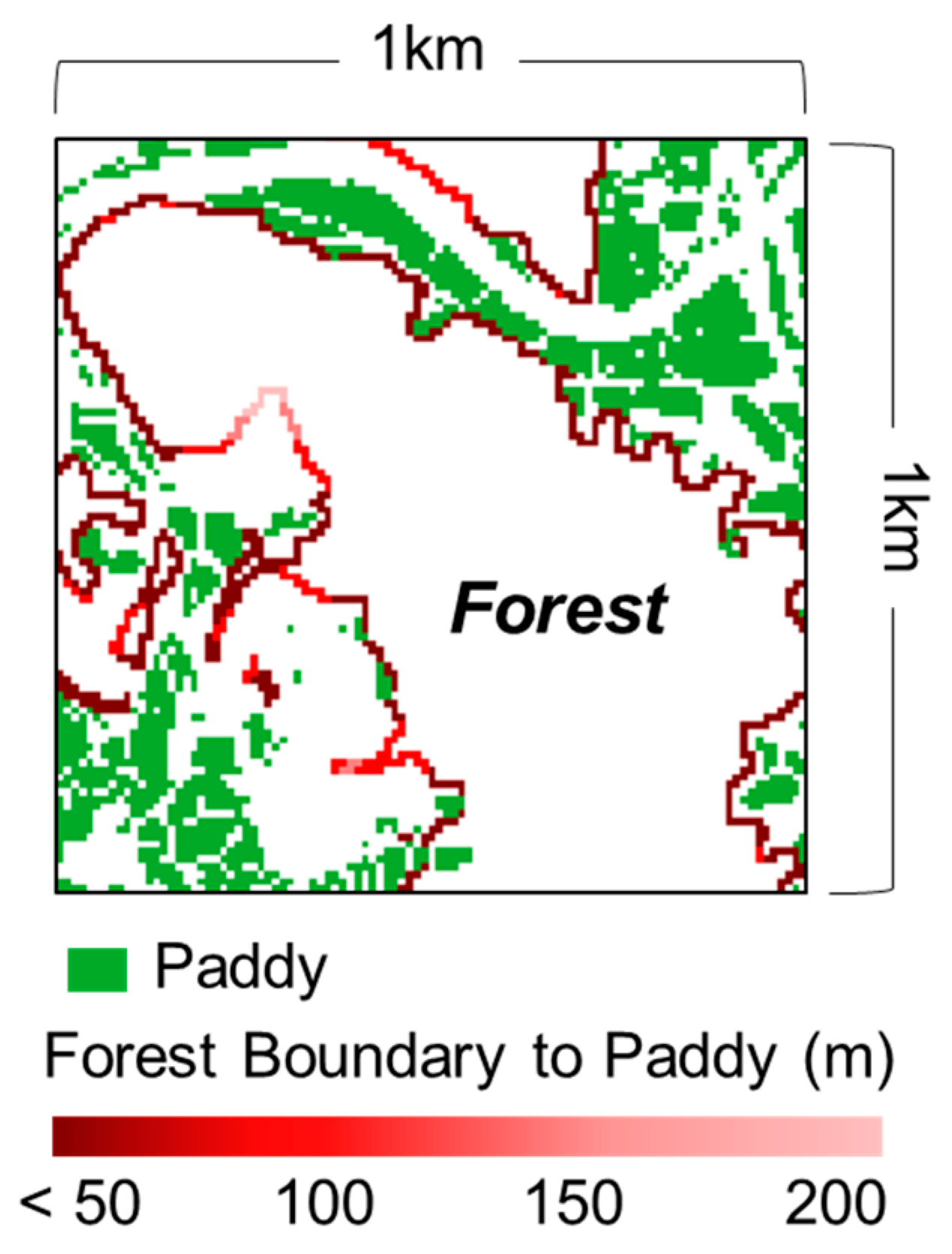
2.1. Study Area

With more than 60% of its land covered by forests, South Korea experiences frequent forest fires, with 562 forest fire events burning an average of 1863 ha annually over the last 5 years [24]. Located at the peninsular in the mid-latitude of Eastern Asia, South Korea is affected by a warm monsoon climate which leads to great seasonal climate variation. Dry weather continues from winter to spring, during which the lack of precipitation and warm springtime temperatures contribute to forests extremely vulnerable to fires, while more than 60% of the 1200 mm of annual precipitation occurs during the hot rainy summer season [4]. Therefore, most forest fires occur from February to April due to a combination of climate (dry, warm weather) and human factors, especially near the Seoul and south-eastern metropolitan areas (Figure 1). In addition, humidity is affected by the mountain chain found from the north to the south on the eastern portion of the Korean Peninsula. Wind blowing from the north-east continent in spring becomes much drier as it passes over the mountain chain and causes large-scale forest fires in the east coastal area [25]. Based on correlation between historical meteorology and recorded forest fires, both the frequency and scale of forest fires in South Korea are expected to increase due to climate change [13].

2.2. Datasets Used

2.2.1. National GIS Data

The forest fire dataset produced by the Korean Forest Service includes burned area, start and end dates, ignition source, and address information for each forest fire event. In this study, all forest fire events from the dataset which occurred during the study period of January 2016 to March 2022 were selected for a total of 3511 forest fire events. We further prepared the dataset for use by geolocating each event. The 1 km-by-1 km gridded population density was collected from the National Geographic Information Institute of Korea, and other datasets were adjusted to fit this resolution. The spatial distribution of agricultural land, which was acquired from the Farm Map produced by the Ministry of Agriculture, Food and Rural Affairs, was also adjusted to the 1 km-by-1 km grid resolution.

2.2.2. Meteorological Data

Daily meteorological data were downloaded through the API service from three different government agencies: the Korea Metrological Agency (KMA), the Korea Forest Research Institute, and the Rural Development Agency (

Table A1. Source of Dataset.

Dataset	Source (Accessed on 25 January 2023)
Forest fire dataset	https://www.data.go.kr/data/3062614/openapi.do
Gridded population density	http://map.ngii.go.kr/ms/map/NlipMap.do?tabGb=total
Meteorological dataset
(Korea Metrological Agency)	https://data.kma.go.kr/data/grnd/selectAsosRltmList.do?pgmNo=36
(Korea Forest Research Institute)	https://know.nifos.go.kr/know/service/list/mtWeatherInfo.do
(Rural Development Agency)	http://weather.rda.go.kr/w/weather/observation.do
Farm map	http://data.nsdi.go.kr/dataset/20210707ds00001
MOD11A1	https://developers.google.com/earth-engine/datasets/catalog/MODIS_061_MOD11A1
MOD13A2	https://developers.google.com/earth-engine/datasets/catalog/MODIS_061_MOD13A2

). The data were collected from 1209 stations, with each station covering approximately 88 km² of land on average, and interpolated for mean and max temperature, precipitation, wind speed, and relative humidity. A lightning observation dataset produced by the KMA was used to calculate the lightning frequency. The processing of lightning data is described in Section 3.1.

2.2.3. Fuel Modeling Data

The fuel load was computed by the multiplication of the above ground biomass (AGB, t/ha) by the ratio for litter ($R^l$, Ct/ha) and deadwood components ($R^d$, Ct/ha) according to the following equations, where AGB is a multiplication of the stock volume (V, m³/ha), the basic woody density (WD, t/m³), and biomass expansion (BEF):

$$\mathrm{Fuel}=\mathrm{AGB}\ast \left(R_t^l+R_t^d\right),$$

(1)

$$\mathrm{AGB}=V\ast {\mathrm{WD}}_t{\ast \mathrm{BEF}}_{\mathrm{t}}$$

(2)

where t indicates a group of major tree species such as Pinus densiflora (Gangwon), Pinus densiflora (Midland), Pinus koraiensis, Larix kaempferi, Quercus variabilis, Quercus monglica, Quercus variabilis with Pinus densiflora, and Quercus monglica with Pinus densiflora. The spatial dataset of the stock volume (V) was derived from the study led by Hong [26] including tree species labeling, and the parameters WD, BEF, $R^l$, and $R^d$ were referenced from the previous literatures [27,28]. The fuel load calculation was based on an assumption that each 1 km² grid is fully occupied by one or two of the aforementioned major tree species in South Korea. This assumption was made because the site index, a measure of site productivity for a given forest stand, is evaluated based on the dominant trees at the Chapman–Richards equation [29], which was used for producing dataset V.

2.2.4. Remote Sensing Data

In addition, remote sensing-based land observation data were collected for the land surface temperature (LST) and vegetation index from the NASA Moderate Resolution Imaging Spectroradiometer (MODIS) products using Google Earth Engine. Daily LST was acquired from MOD11A1 and masked for cloud-free areas with the quality band. As the vegetation index changes relatively slowly compared to temperature, a normalized difference vegetation index (NDVI) was acquired from MOD13A2 with 16-day composite imaging to minimize the noise in the time series dataset; it was then reconstructed to daily data with the algorithm proposed by Chen [30]. Accessible links for the used dataset can be found in Table A1.

3. Methods

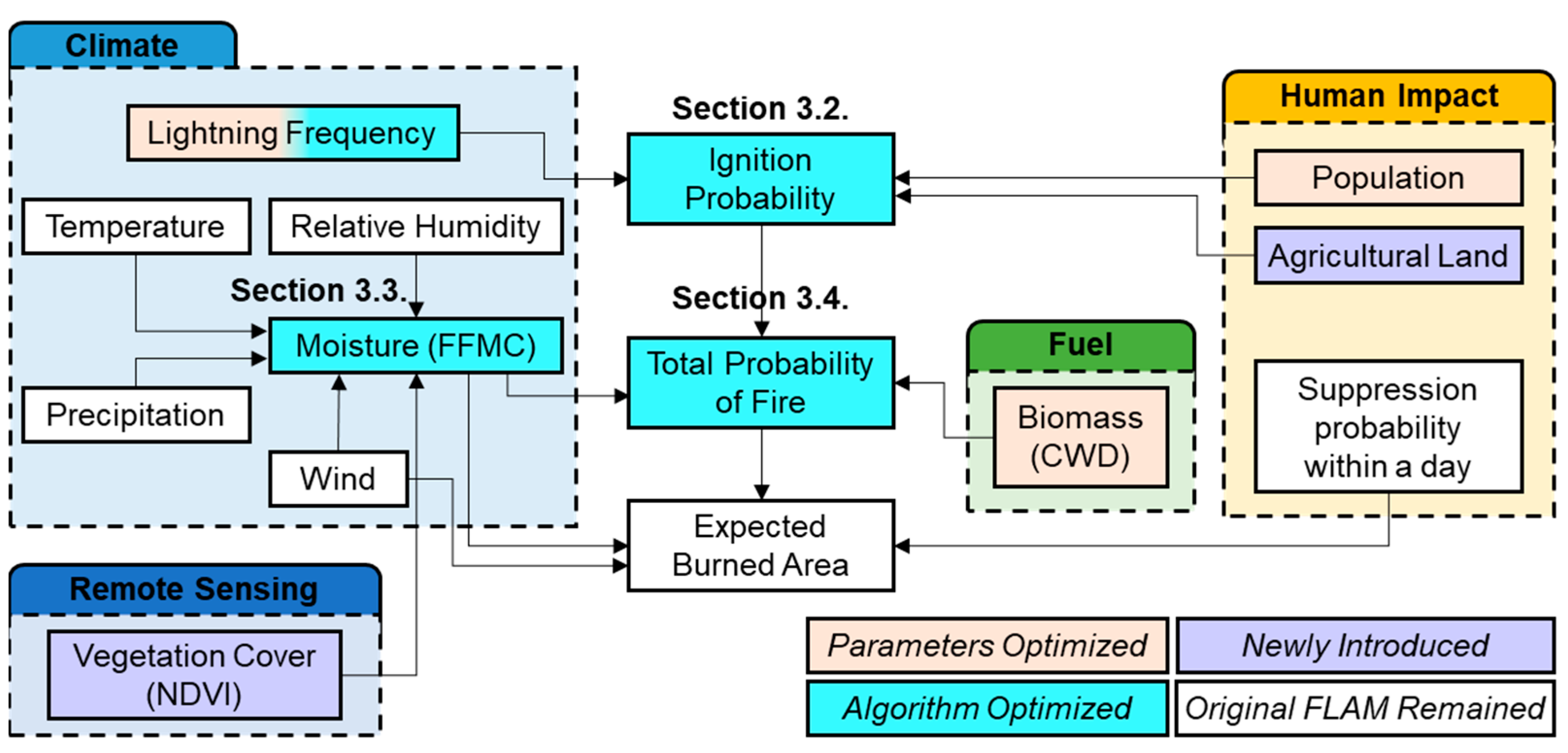
3.1. Forest Fire Model Developed by IIASA

FLAM is a process-based model developed by IIASA that contains parameterization algorithms for capturing the impacts of climate, population, and fuel availability on the forest fire frequency and burned area on a global scale (Figure 2). FLAM calculates the ignition probability from both human and natural sources. The probability of fire occurrence is calculated using daily weather conditions and fuel availability in each grid cell. FLAM uses the climate data for the following variables—temperature, precipitation, wind speed, and relative humidity—to compute the fuel moisture content based on the Fine Fuel Moisture Code (FFMC) of the Canadian Forest Fire Weather Index (FWI) [31]. Fuel available for burning is defined as a combination of litter and coarse woody debris (CWD) from the above-ground biomass, excluding the stem biomass. For areas with a positive probability of fire, the expected burned area is calculated by simulating fire spread due to wind speed, fuel moisture, and the fire suppression efficiency, which is implemented as the probability of extinguishing a fire on a given day.

One of the key features of FLAM is a procedure to calibrate the spatial fire suppression efficiency to better capture the inter-annual dynamics of the historical areas burned. The spatial variability of the suppression efficiency can be explained by the effects of infrastructure and management over the processed biophysical impacts and probability of fire. Previously, FLAM aimed to simulate the burned area and demonstrated a good agreement with the historical burned area reported in Europe and Indonesia [22,32]. A specific modeling of the forest fire frequency in relation to regional environmental factors is important [33] as it would help to assess the impact of infrastructure and management on the burned area.

Our goal was to improve the simulation of the forest fire frequency and burned area in South Korea. Therefore, this study optimized the algorithms for interpreting anthropogenic and biophysical factors to improve the calculation of the ignition probability and the total probability of fire. To enhance spatial details on the fuel moisture calculation, this study also introduced remote sensing-based vegetation cover and adjusted the algorithm to represent the soil moisture dynamics observed from the satellite data. The impact of proximity to agricultural land was introduced in FLAM to model the seasonal patterns of the forest fire frequency in South Korea.

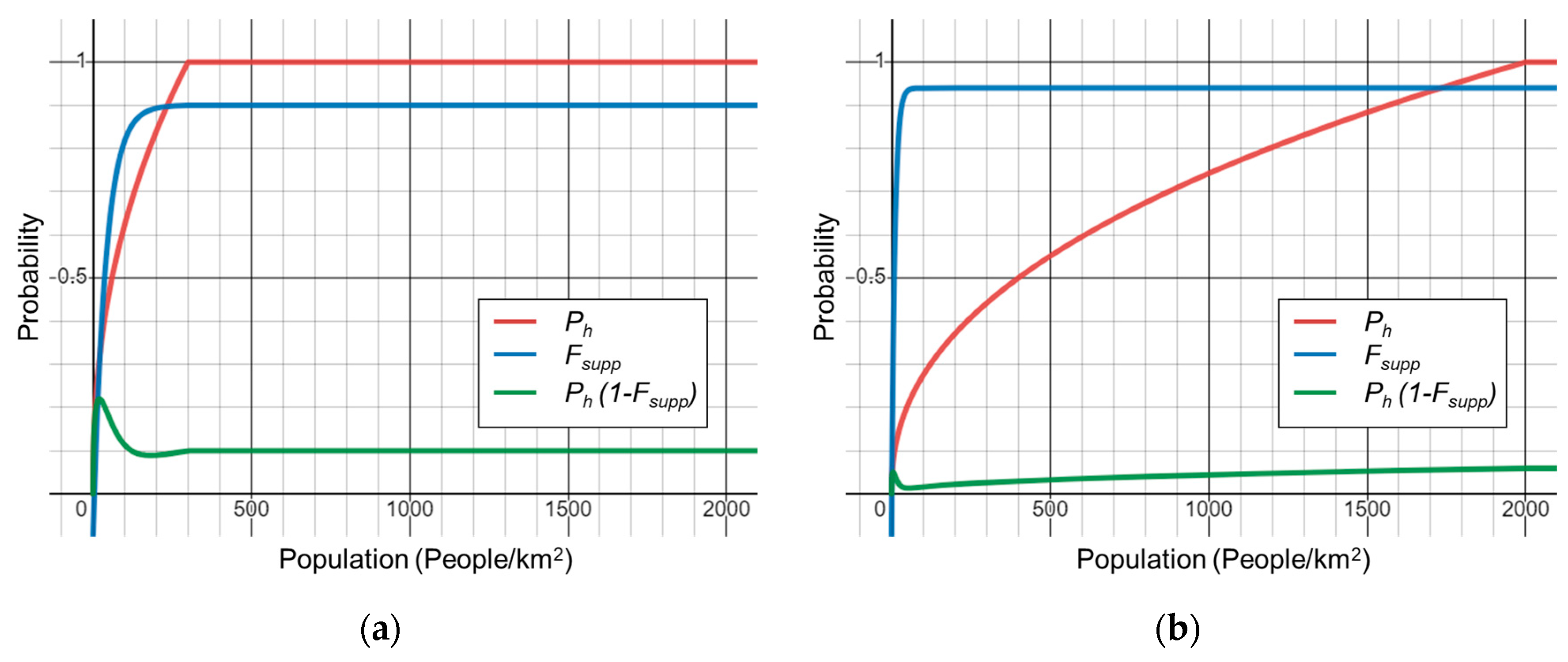
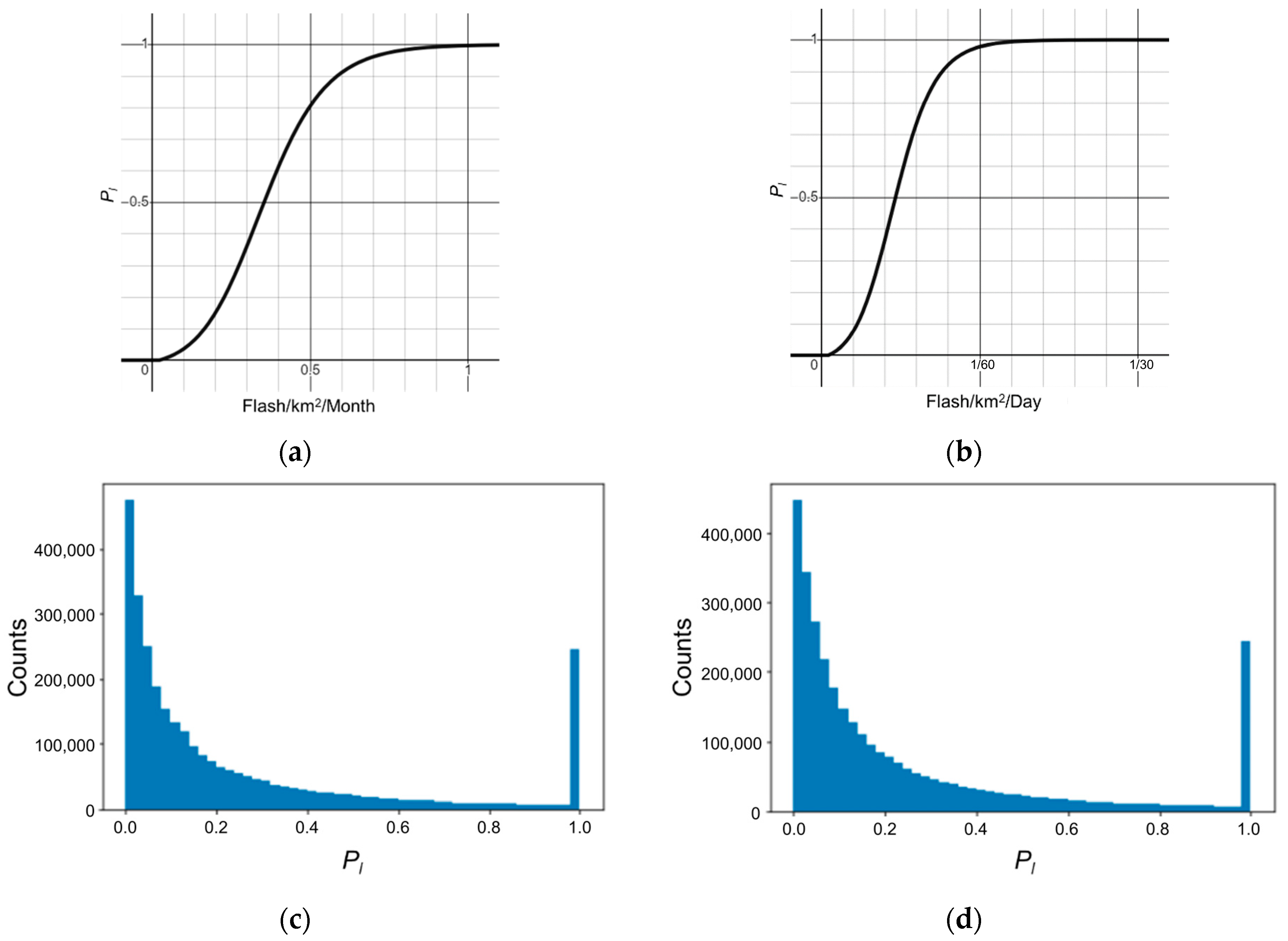
3.2. Ignition Probability

Our analysis of the constructed forest fire dataset shows that 61.98% of forest fires started as a result of human activities during the study period: 10.08% from agricultural waste burning, 12.33% from waste burning, 32.64% from negligence, 0.17% from arson, and 6.75% spread from building. Only 0.06% of forest fires were caused by lightning, and the cause(s) of the remaining 37.67% fires were not recorded. Forest fire frequency increases exponentially with proximity to metropolitan cities, where a high population density combines with lower humidity as a result of several factors, such as urbanization, seasonal variation, and climate change [14,34]. In this way, South Korea is similar to Europe, where human activity is a major cause of forest fires [35]. However, metropolitan cities in South Korea such as Seoul and Busan have much higher population densities than cities in Europe: 15,699 and 4320 people per km² covering areas of 605.2 and 770 km², respectively.

Therefore, we improved the ignition probability of FLAM by optimizing the parameters of human ignition factors to represent the dominant ignition frequency near highly populated cities. In FLAM, human impacts are modeled as a combination of human ignition probability (P_h) and suppression probability (F_supp) as follows:

$$P_h=\min (1,{\left(\frac{p}{p_{up}}\right)}^{0.43}),$$

(3)

$$F_{supp}=1-\left((1-Sup{p}_{max}\right)+\exp (-C_{supp}\ast p)),$$

(4)

where p_up, Supp_max, and C_supp indicate the upper threshold of population density, maximum probability of instant suppression, and suppression coefficient of population density, respectively. Therefore, P_h does not further increase when the population density surpasses p_up, and F_supp reaches Supp_max as the population density increases while its rate is controlled by C_supp.

In this study, P_h was adjusted by increasing p_up from the default value of 300 people per km² to 2000 people per km². This value was increased because the default value was exceeded in most of the cities, which account for 7.7% of the land area and have a maximum population density of 45,739 people per km². Meanwhile, Supp_max and C_supp were increased to represent the faster response system found in South Korea, which has a higher standard to follow as compared to other countries of the world [36,37].

In addition to the human factor, the probability of natural ignition (P_l) is calculated in FLAM from monthly lightning frequency data (L_f) and combined with the human ignition probability P_h to evaluate the total ignition probability (P_i) according to the following equations:

$$B_L=\max \left[0,\min \left(\frac{L_f-L_{f,low} }{L_{f, up}-L_{f, low}}\right)\right]$$

(5)

$$P_l=\frac{B_L}{B_L+\exp \left(1.5-6B_L\right)}$$

(6)

$$P_i=\left(P_l+\left(1-P_l\right)P_h\right)\left(1-F_{supp}\right),$$

(7)

where $B_L$ represents the normalized value of monthly lightning strikes L_f per km² to a value from 0 to 1, based on L_f,low and L_f,up, which are set to 0.02 and 0.85, respectively, as default values. However, the current calculation of lightning with a monthly time step inevitably overestimates the number of forest fires caused by lightning, because other biophysical factors—in particular, the fuel moisture content—are computed with a daily step. As described above, more than 50% of the annual precipitation in South Korea occurs in the summer. The monthly lightning frequency peaks in the rainy summer season, rarely developing into a forest fire due to high precipitation. However, when integrated with daily fuel moisture, which is likely to include dry summer days, the probability of fire is overestimated, as illustrated in Figure 3.

Given that only 0.06% of historical forest fires were caused by lightning, neglecting lightning ignition is unlikely to significantly affect the results in the current environment. However, as the ultimate goal of modeling is to project forest fires in the future, which will be accompanied by significant environmental changes, this study also optimized lightning ignition probabilities. To correct the overestimated ignition by lightning, the algorithm for lightning frequency was changed from a monthly to a daily time step, and parameters L_f,low and L_f,up were optimized in such a way that the daily probability maintains the distribution of the monthly probability. As the lightning dataset is acquired for each lightning event at an exact location, the lightning frequency was calculated with the focal statistics tool in ArcGIS software with a focal radius of 17,841.24 m, equivalent to 1000 km², the same scale as the FLAM algorithm (see Section 3.4). In addition, the number of historical forest fires caused by lightning strikes was referenced to optimize the normalization parameters. Although only two forest fires were recorded as having been caused by lightning, the parameters were optimized to return little overestimation, implying that some of the forest fires with an unknown cause in the database could have been caused by lightning.

Warm and dry weather during the spring season of South Korea results in a special pattern of forest fires, with more than 60% concentrated in a quarter of the year, from February to April. However, the fire season results not from dry weather only but also from the national custom of burning agricultural waste, such as agricultural plastic waste and leftover plants after the harvest. According to the dataset, 10.08% of forest fires in the study period were directly caused by the burning of agricultural waste, and this proportion increased to 22.42% when the recorded ignition source ‘burning waste’ was included. Both ignition sources increase exponentially throughout the spring season, when agricultural lands are cleared for the consequent planting, and the increasing proportion to the other ignition sources indicates that the increasing number is not attributed solely to dry weather (Figure 4).

Therefore, agricultural waste burning was introduced to FLAM as a new ignition factor to fit the specific pattern of forest fires in South Korea. The newly introduced ignition probability conditional on agricultural waste burning (P_a) was calculated as a function of the forest boundary neighboring an agricultural field. As the calculation is processed in grid format, the number of grids with a 10 m resolution located at the forest boundary and neighboring agricultural field within 200 m for a 50 m interval was acquired for each 1 km² area (Figure 5). Then, the P_a for each 1 km² pixel was calculated according to the following equation:

$$\begin{gathered} P_a=1-{\left(1-w_m\ast r_{\le 50}\right)}^{N_{\le 50}}\ast {\left(1-w_m\ast r_{\le 100}\right)}^{N_{\le 100}} \\ \ast {\left(1-w_m\ast r_{\le 150}\right)}^{N_{\le 150}}\ast {\left(1-w_m\ast r_{\le 200}\right)}^{N_{\le 200}} \end{gathered}$$

(8)

where N_≤50, N_≤100, N_≤150, and N_≤200 represent the number of 10 m grids within 200 m for a 50 m interval, and r_≤50, r_≤100, r_≤150, and r_≤200 are the weights for each distance. The newly defined ignition probability P_i after the inclusion of agricultural waste burning is extended from Equation (7) as follows:

$$P_i=\left(P_l+\left(1-P_l\right)P_h+\left(1-P_l-P_h\right)P_a+P_l{P}_h{P}_a\right)\left(1-F_{supp}\right),$$

(9)

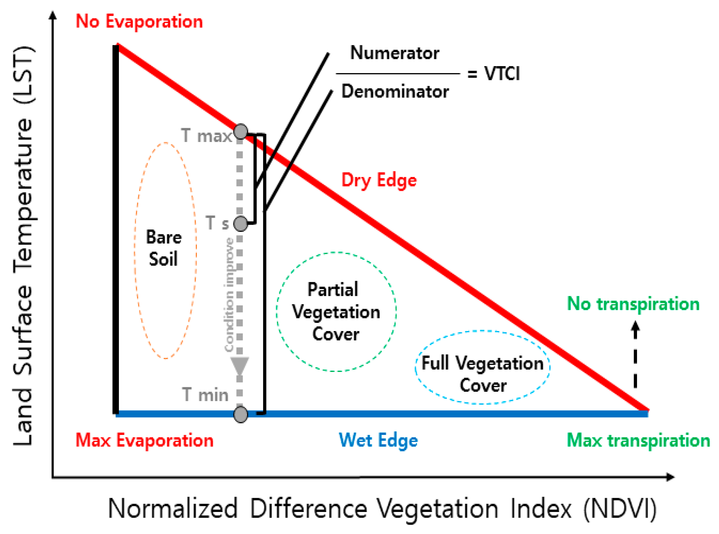
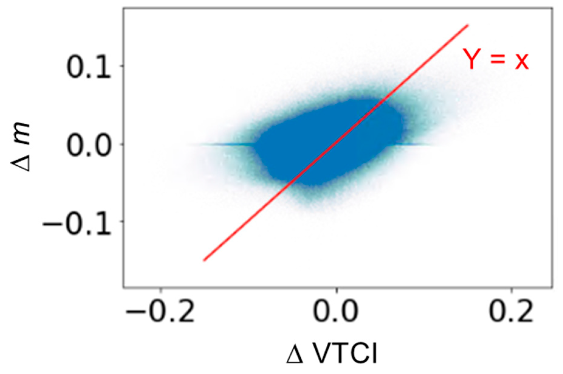
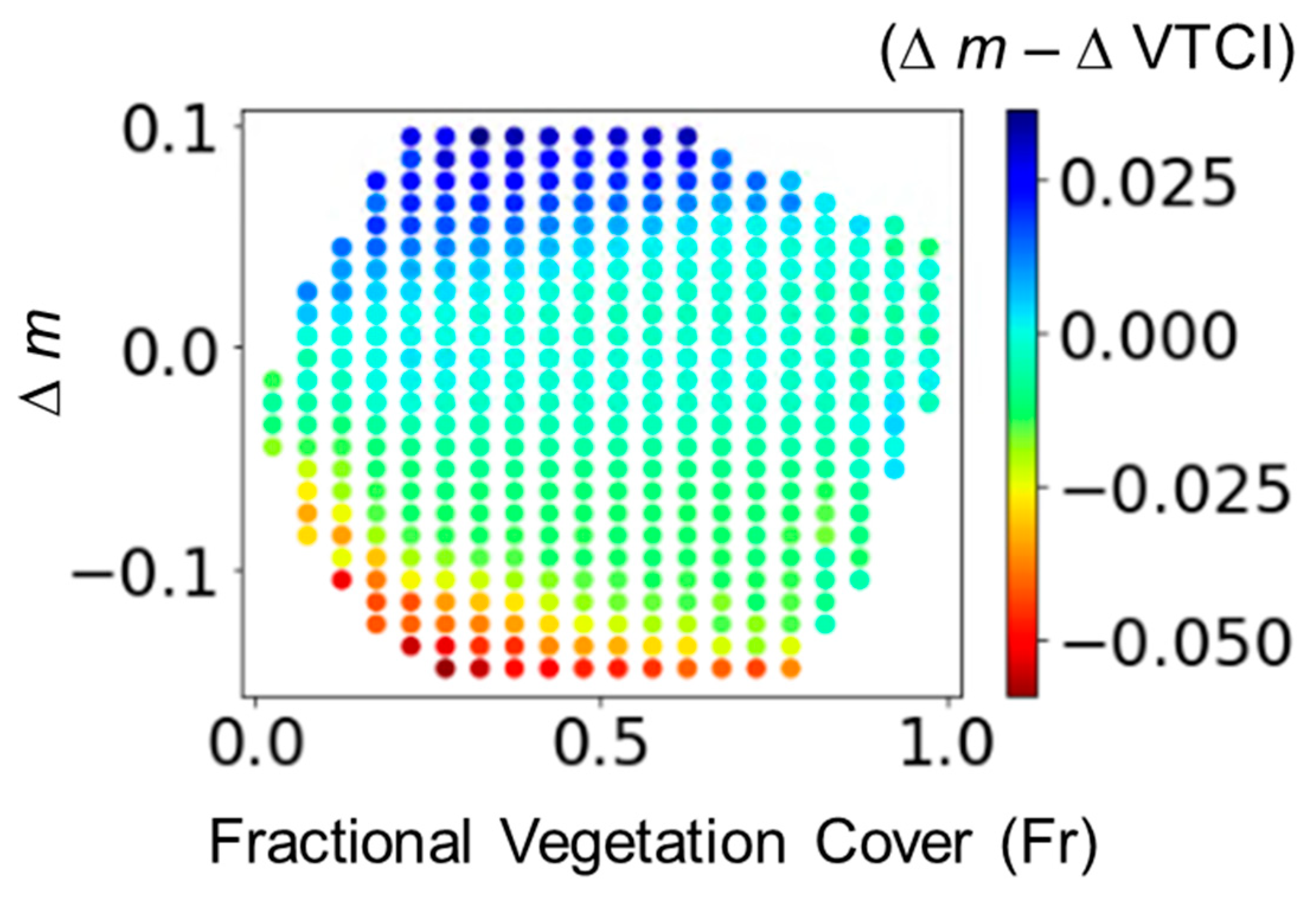
3.3. Fuel Moisture Content Calculation

The daily fuel moisture content (m) is calculated by using FFMC (V_FFMC), which is one of the key factors in FLAM to project both the forest fire frequency and burned area under a changing climate. As a component of the FWI, the FFMC evaluates the litter and cured fine fuel layer in the top 1.2 cm of soil for the relative ease of the ignition and flammability of fine fuels [38]. The FFMC is calculated with the daily temperature, precipitation, wind speed, relative humidity, and the m of the previous day. The FFMC ranges from 0 to 100, with higher values meaning more flammability, while m ranges from 0 to 250% (the detailed formulation of the FFMC be found in Appendix B).

$$m=f_m\left(V_{FFMC}\right)=\frac{0.01\left(59.5\ast 250-147.2\ast V_{FFMC}\right)}{V_{FFMC}+59.5}$$

(10)

In this study, the daily FFMC was calculated using the domestic meteorological dataset at a 1 km resolution, enabling a more precise representation of the regional variations of parameter m. However, the current FFMC algorithm has limitations because it only exploits meteorological information and ignores the explicit interaction between weather and the land surface environment.

To overcome the limitation of purely meteorological modeling, a framework for comparing the results of meteorological modeling with the land surface observations was proposed to identify and exploit the empirical differences [23]. In this study, we also aimed to improve the calculation process of the FFMC by fitting the daily parameter values of m to the remotely sensed soil moisture, and by deriving an empirical equation of their difference explained by the land surface characteristics.

We compared the moisture content m with the Vegetation Temperature Condition Index (VTCI), a satellite-based index representing the topsoil moisture by interpreting LST-NDVI feature space [39]. The VTCI is calculated based on the ratio of LST normalized by NDVI in between the upper (dry edge) and lower (wet edge) limits of the data boundary (Figure 6). The VTCI ranges from 0 to 1 for the dry and wet edge, respectively, corresponding to the minimum and maximum evapotranspiration. Similar to the FFMC, which assesses the fuel moisture content at the top 1.2 cm surface layer, the VTCI has a positive correlation with the soil moisture content in the surface layer [40].

Since the moisture content m is calculated from the meteorological conditions of the current day (M_t) and the previous day (m_t−1) values, m and the VTCI were compared by replacing the previous m with the previous VTCI (Equation (11)). As m and the VTCI cannot be compared at the same scale, the iso-value lines of the VTCI were optimized between the two edges. The iso-value line can adjust the scale of the VTCI and determine the way of interpreting the LST-NDVI feature space, so that the VTCI value can better represent the moisture in a specific layer [41], such as fuel in the surface layer.

$$m=f_m\left(V_{FFMC, t}\right)=f_m\left(f_{FFMC}\left(m_{t-1}, M_t\right)\right)\fallingdotseq f_m\left(f_{FFMC}\left(f_{iso}\left(V_{VTCI, t-1}\right), M_t\right)\right)$$

(11)

In addition, both the daily mean temperature and daily maximum temperature were tested for the FFMC calculation to discover which method better represents the daily forest fire pattern while the original algorithm for the FFMC calculation uses meteorology at noon.

3.4. Probability of Fire

The ignition probability was calculated in Section 3.2 from human and natural sources, and in conjunction with biophysical factors such as fuel availability and fuel moisture, the probability of fire was determined.

In FLAM, the ignition probability conditional on fuel availability (P_b) was calculated by normalizing the amount of fuel (B) as follows:

$$P_b=\max \left[0,\min \left(1, \frac{B-B_l}{B_u-B_l}\right) \right]$$

(12)

where B_u and B_l are the maximum and minimum boundaries of the probability, set to 200 gC/m² and 1000 gC/m² as a baseline, respectively. In this study, the parameters B_u and B_l were optimized to broaden the normalization boundary because the distribution of B increases in data at a higher spatial resolution, with a more precise representation of environmental heterogeneity at a local scale.

The daily probability of ignition conditional on fuel moisture (P_m) is calculated according to the following equation:

$$P_m=1-tanh{\left(1.75\ast \frac{m}{m_e}\right)}^2,$$

(13)

where m_e is the moisture of extinction set to 0.35 as a baseline. In this study, m_e was optimized to reproduce the seasonal pattern of the forest fire frequency in South Korea.

Then, the total probability of fire (P) is calculated by the multiplication of the conditional according to the following equation:

$$P=P_i\ast P_b\ast P_m$$

(14)

However, it should be noted that the equation for the probability of fire was originally designed on a 1000 km² scale and extrapolated when applied to a larger spatial resolution [15]. Extrapolation to a larger resolution can be performed by multiplying the targeting resolution divided by 1000 km², which produces P for the included sub-areas of 1000 km²; for example, if the larger area is 5000 km², one needs to multiply by 5, i.e., 5000/1000. However, when P needs to be interpolated to finer resolutions, simple multiplication will no longer apply because there would be no sub-areas less than 1000 km². Therefore, the optimization process to a scale of 1 km² was proposed in this study. Considering that the original probability of fire (P^L) indicates the probability of more than 1 fire in 1000 km², it can be expressed by the complementary event of no forest fire in every 1000 areas of 1 km² inside the 1000 km² pixel. This can be expressed as follows:

$$P^S=1-\sqrt[1000]{1-\left(P_i\ast P_b\ast P_m\right)}.$$

(15)

Thus, downscaling the probability of fire to 1 km² (P^S) can be statistically derived through the equation when all subordinating areas share the averaged environmental factors of the 1000 km² area. However, in a practical application, P^S varies for each location because the downscaled dataset can represent heterogeneous environments. P^S should be calibrated to reflect forest fire dynamics at a scale of 1 km² in addition to the statistical downscaling described above. In this study, the calibration multiplicator (C_calib) and spatio-temporal dependency between adjacent areas were introduced for modeling smoldering fires and horizontal fluxes that might occur as follows:

$$Step1: P^S=1-\sqrt[1000]{1-\left(C_{calib}\ast P_i\ast P_b\ast P_m\right),}$$

(16)

$$Step2: P^S=\frac{{{\displaystyle \sum }}_j\left(w_j\ast P^{S,j}\right)}{{{\displaystyle \sum }}_j{w}_j},$$

(17)

$$Step3: P^{S,t}=1-\left(1-P^{S,t}\right)\ast \left(1-C_{recur}\ast P^{S,t-1}\right),$$

(18)

where j and t indicate the adjacent 9 pixels in a 1 km² resolution and the projected time in a daily time step, respectively, and C_recur is the rate of forest fire recurrence within one day. The spatial weight (w) is derived based on adjacency using the distance-weighted mean algorithm:

$$w_j=\frac{1}{{{\displaystyle \sum }}_k\left|d_{j,k}\right|},$$

(19)

where k is the location of the adjacent nine pixels other than j and d_j,k is the distance between j and k.

4. Results

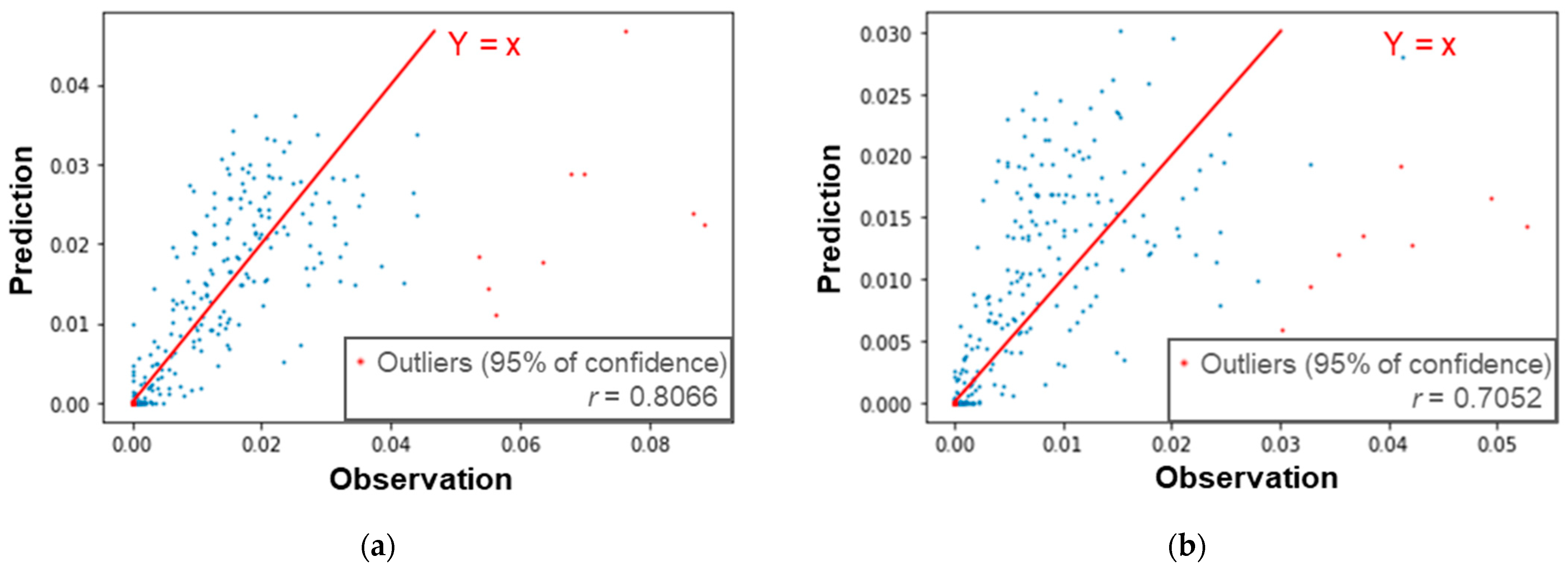
4.1. Optimized Probability Equations

Table 1. FLAM parameters optimized in South Korea.

	Human			Lightning		Fuel		Fire
	Pup	Suppmax	Csupp	Lf,low	Lf,up	Bl	Bu	Me	Ccali	Crecur
Global scale	300	90	0.025	0.02	0.85	200	1000	0.35	-	-
Optimized	2000	94	0.100	0.02	0.55	0	2000	0.32	30	0.0067

P_up: upper threshold of population density (people per km²), Supp_max: maximum probability of instant suppression. C_supp: suppression coefficient of population, B_l and B_u: lower and upper boundaries of fuel (gC/m²). L_f,low & L_f,up: lower and upper boundaries of monthly lightning strikes (strikes per km²). M_e: moisture of extinction, C_cali: calibration multiplicator, C_recur: rate of forest fire recurrence within one day.

presents the original and optimized parameters of FLAM for South Korea, which were obtained by examining Pearson’s correlation coefficient (r) between FLAM and observed data for the period between January 2016 and December 2019. The remaining dataset was not considered during the optimization process to prevent and analyze overfitting. According to the results produced during optimization, the human impact on forest fire ignition was increased in densely populated areas by raising the upper threshold of the population density, while the probability of unsuppressed ignition in a sparsely populated area was decreased by increasing the probability of instant suppression (Figure 7).

The probability of ignition P_l was optimized by changing L_f,up from a value of 0.85 to 0.55. No changes were made to the value of L_f,low. Even though this optimization maintained the original distribution of P_l as illustrated in Figure 8, the frequency of forest fire ignited by lightning changed from 1874.61 to 6.53 times within the study period. This accurately reflects the recorded number of forest fires caused by lightning.

The newly introduced probability P_a was calculated by setting a weight for zones between a forest boundary and an agricultural field in 50 m intervals from 0 to 200 m based on the ratio of forest fires in each zone and a weight for each month, based on the historical pattern of forest fire frequency. The distance weights, r_≤50, r_≤100, r_≤150, and r_≤200, were set to 0.46845, 0.42829, 0.18948, and 0.13902, respectively [42]. The monthly weight, w_m, was set to 0.00035 for January and 0.0012 for both February and March.

By fitting the iso-value lines of the VTCI using Equation (11), the scale of m and the VTCI were matched in such a way that the daily fuel moisture change in both indicators corresponds to each other (Figure 9). As the two different indicators exploit different types of data, a mismatch at a local level is inevitable. However, when the difference between m and the VTCI is projected in the ∆m—fractional vegetation cover (Fr) data space, where Fr is calculated by squared normalized NDVI [43], the fuel moisture increment was greater in the FFMC algorithm as compared to the VTCI, especially when Fr is lower and the changing amount is greater (Figure 10); therefore, the rate of fuel moisture change in the FFMC needs to be slowed down to be compatible with the remotely sensed moisture content.

Thus, the optimization of the FFMC algorithm was achieved by reflecting the effect of Fr and adjusting the overall fuel moisture increment. To reflect the effect of Fr on the fuel moisture increment, the fine fuel equilibrium moisture content (EMC) was calibrated with the first order equation of Fr. After the optimization, a higher Fr decreased the EMC for drying and increased the EMC for wetting, which resulted in a larger increment at higher Fr values. In this stage, fuel moisture of the FFMC changes faster than the VTCI in both low and high Fr conditions. Then, the overall fuel moisture increment of the FFMC was adjusted to 43% of the original algorithm to fit the rate of the VTCI. By optimizing the algorithm with Fr, which is a representative land surface environment with a simple calculation equation, the optimized FFMC can be projected with future conditions along with the simulated Fr.

In addition, using the maximum temperature to calculate m was found to better represent the historical forest fire frequency pattern as compared to using the average temperature. It corresponds to the FFMC calculation manual which encourages using meteorological data at noon, a value that is often equal or similar to the maximum temperature rather than the average temperature. In a similar context, the decrement of m_e can be explained by the overestimation of m because of using a daily average for relative humidity.

The C_recur was set to 0.0067 by the percentage of historical forest fire recurrence in a day within the adjacent pixels.

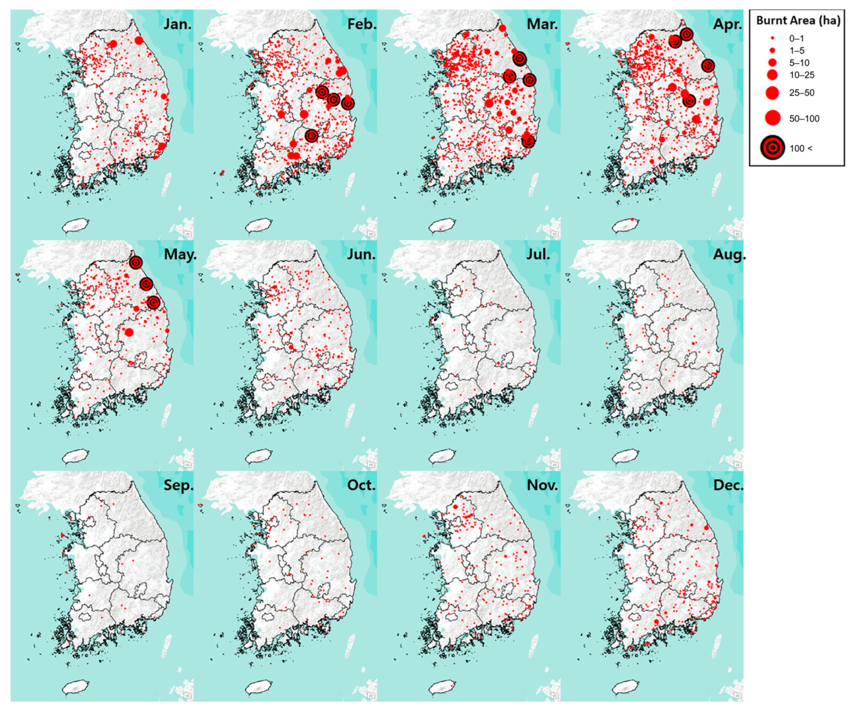
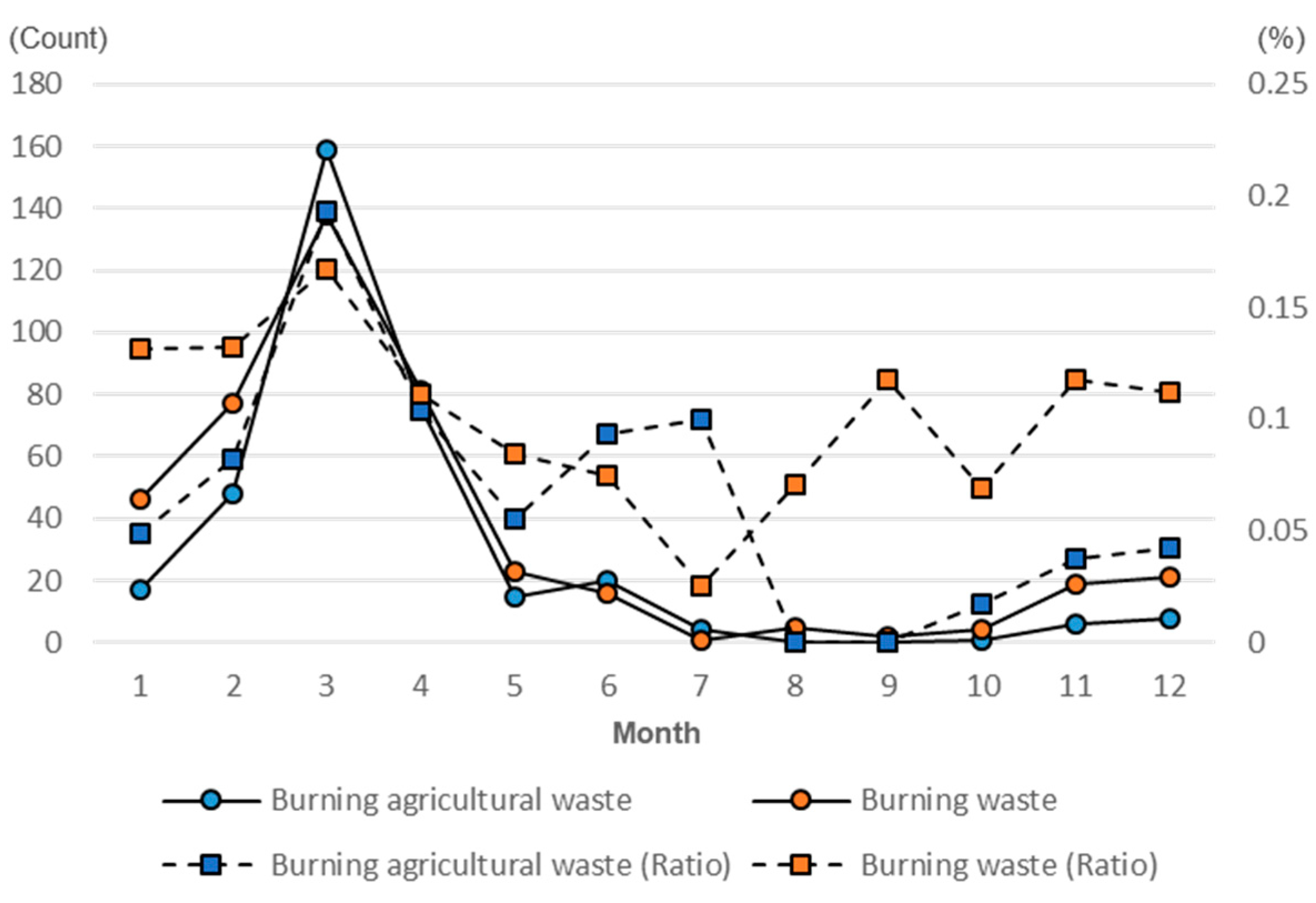
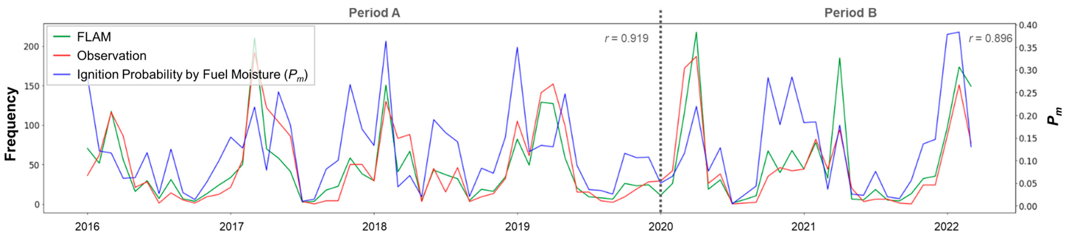
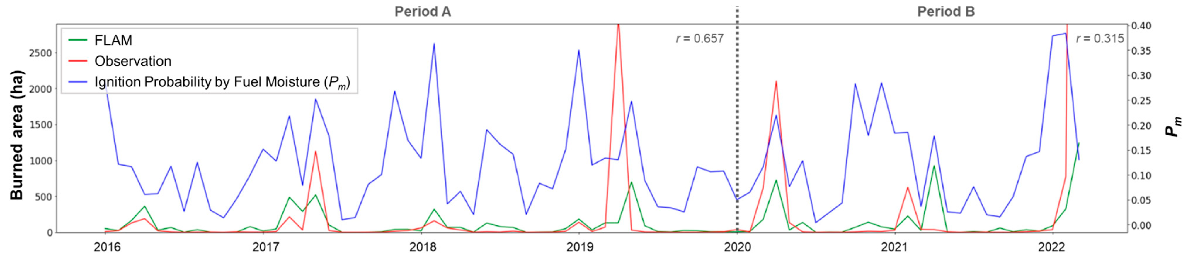
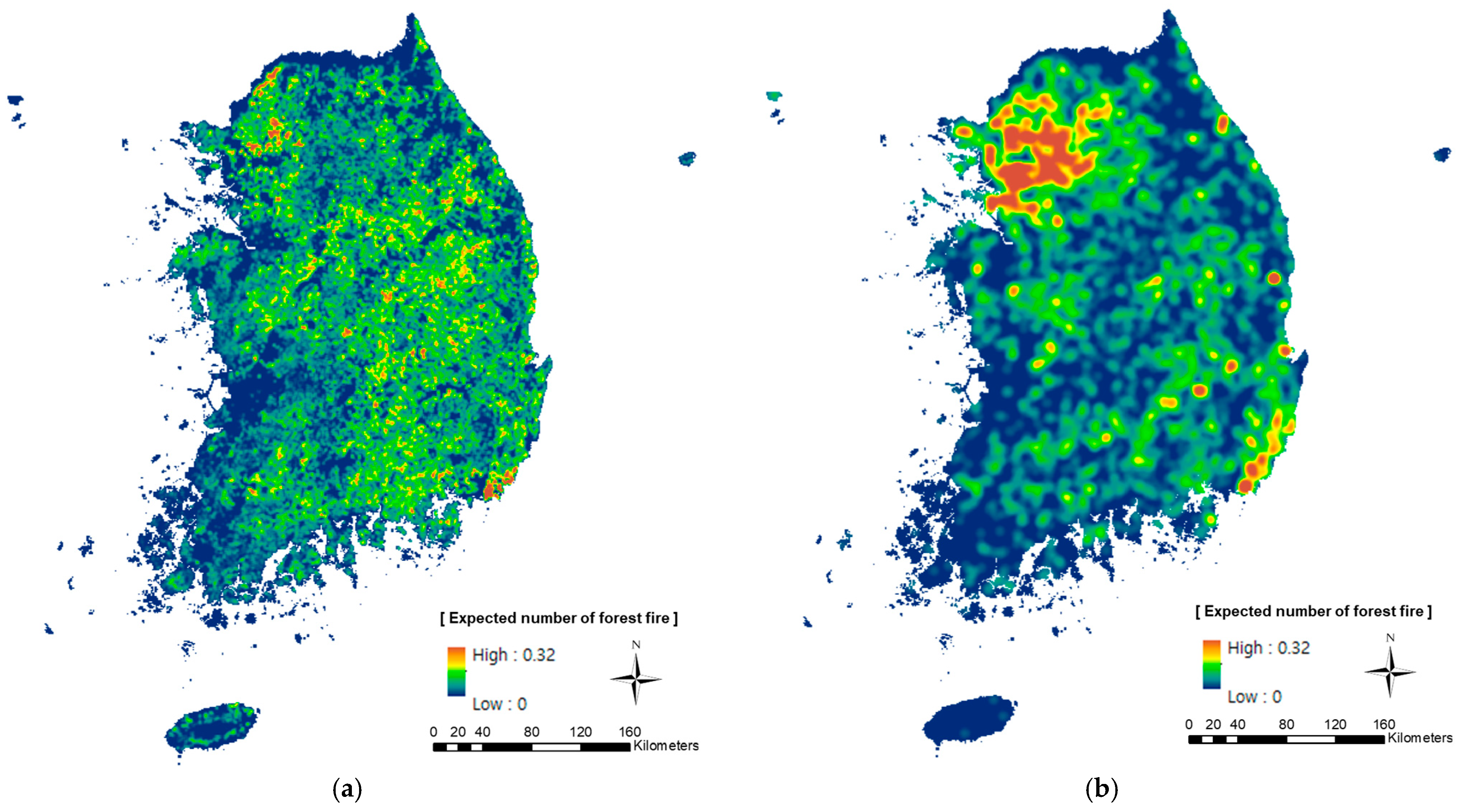
4.2. Simulation of the Historical Forest Fire Events

To validate the optimization performance, the historical forest fire frequency and burned area were simulated using the dataset from January 2016 to March 2022. We used the standard from FLAM without calibrating the suppression efficiency [22]. To assess the performance, Pearson’s correlation coefficient (r) was computed between FLAM simulations and observed data, with the dataset split into two periods: period A, which was used for the optimization (before 2020), and period B (after 2020) to test the model’s generalization over time.

According to the simulation results, a temporal evaluation on the monthly forest fire frequency in period A and B improved the r values of 0.050 and 0.447 to 0.919 and 0.896, respectively, when the optimization condition was changed after applying only statistical downscaling in Equation (15) to the full optimization (Figure 11). A temporal evaluation of the burned area was performed only for the forest fires with a burned area less than 1000 ha per single fire ignition, as this study focused on frequency optimization and applied a global scale optimization method to the burned area, which has a limitation in terms of modeling occasional large-scale forest fires at a local scale. The simulation of the burned area for the periods A and B resulted in r values of 0.657 and 0.315, respectively (Figure 12).

The simulation of the forest fire frequency was also evaluated in a spatial extent by aggregating the frequency value to a 25 km by 25 km grid. Figure 13 shows the spatial evaluation in periods A and B with the grids within a 95% confidence level recording the r of 0.8066 and 0.7052, respectively. The evaluation results show that the optimized FLAM is able to reproduce the forest fire patterns in South Korea, showing good correlation to historical records, particularly for forest fire frequency. The evaluation results did not show a substantial difference between periods A and B. Therefore, the model is expected to be robust with respect to time periods, including possible projections of future fires. However, several outlier grids have been found in the spatial evaluation and all of the outliers were commonly underestimations in the region where a high forest fire frequency was observed.

The underestimated forest fire frequency can be located by comparing the maps of the expected number of forest fires (Figure 14). In the FLAM simulation, the expected frequency of forest fires was calculated as the cumulative sum of P. The observational expected frequency was obtained by interpolating forest fire location points with the kernel density of ArcGIS software, to match the maximum expectation range with FLAM. The result of the optimized FLAM presents a smaller scale of undispersed hotspots near cities as compared to the observations, which indicates that the underestimated outliers were on the outskirts of cities. In addition, the prediction showed a relatively higher value through the linear feature of major mountain chains and near the cities, generating a varied scale of hotspots.

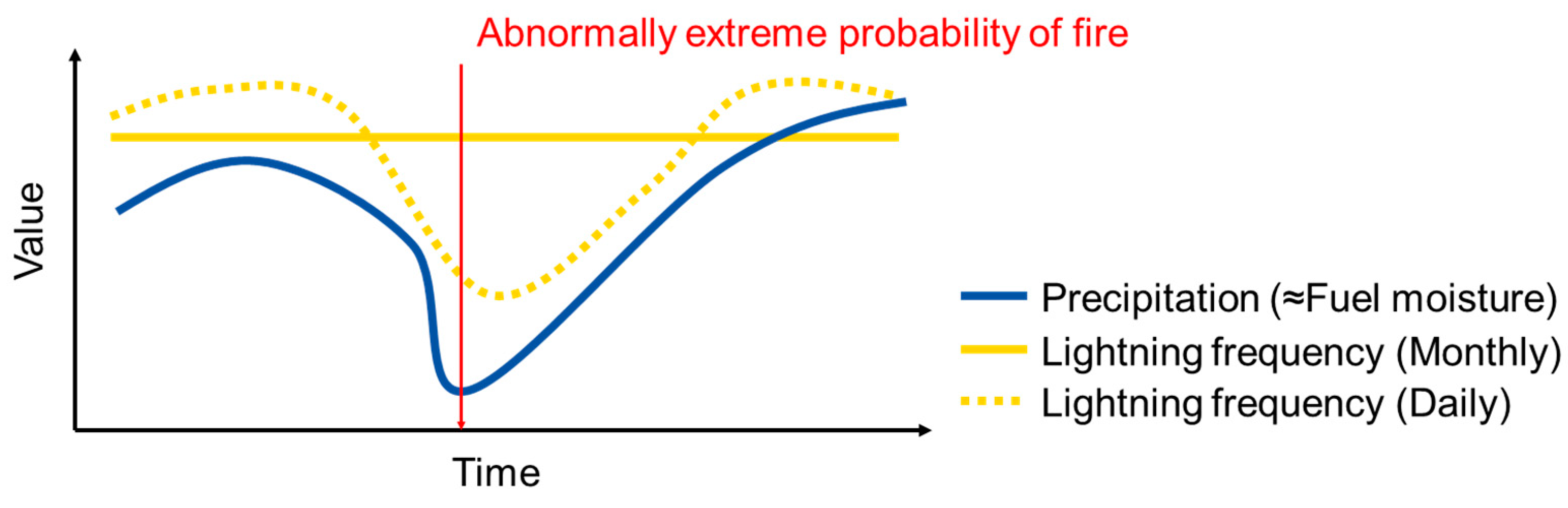
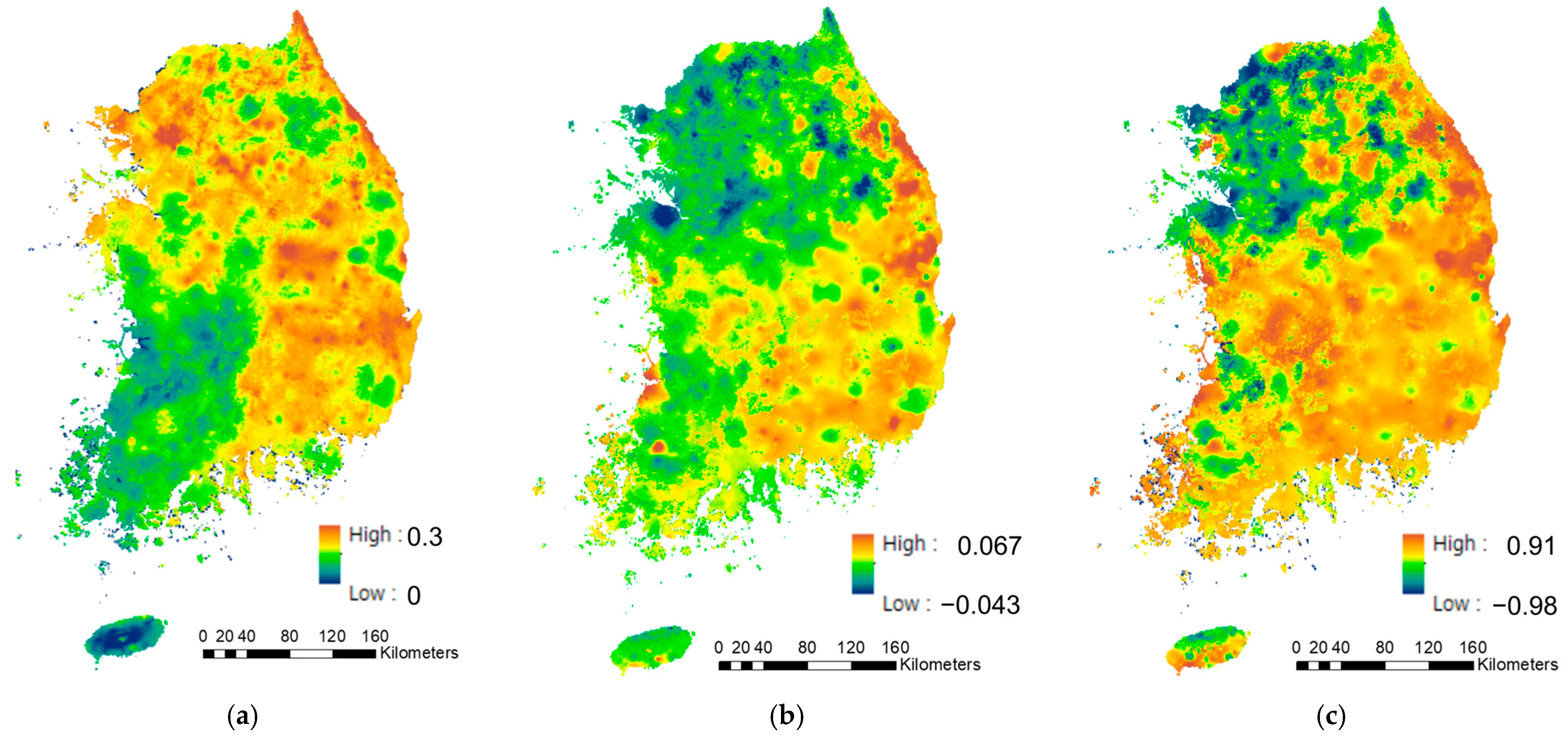
4.3. Trend of Ignition Probability by Fuel Moisture in Spring Season

To further investigate the impacts of P_m, the trend of the optimized P_m in the spring season (January and February) was examined for the observed 7 years (Figure 15). According to the result, the average P_m over the 7 years was relatively high near the Seoul metropolitan area and the east costal area, where frequent and severe forest fires currently occur. Moreover, P_m at the east coastal area increased at a significant level, which implies that the risk of a forest fire will increase in the future in this area, which has already suffered from large-scale forest fires. Even though we may need a longer observation period to confirm these results, we are confident that the risk of a forest fire is increasing as a direct result of climate change, leading to drier fuels in certain regions of South Korea.

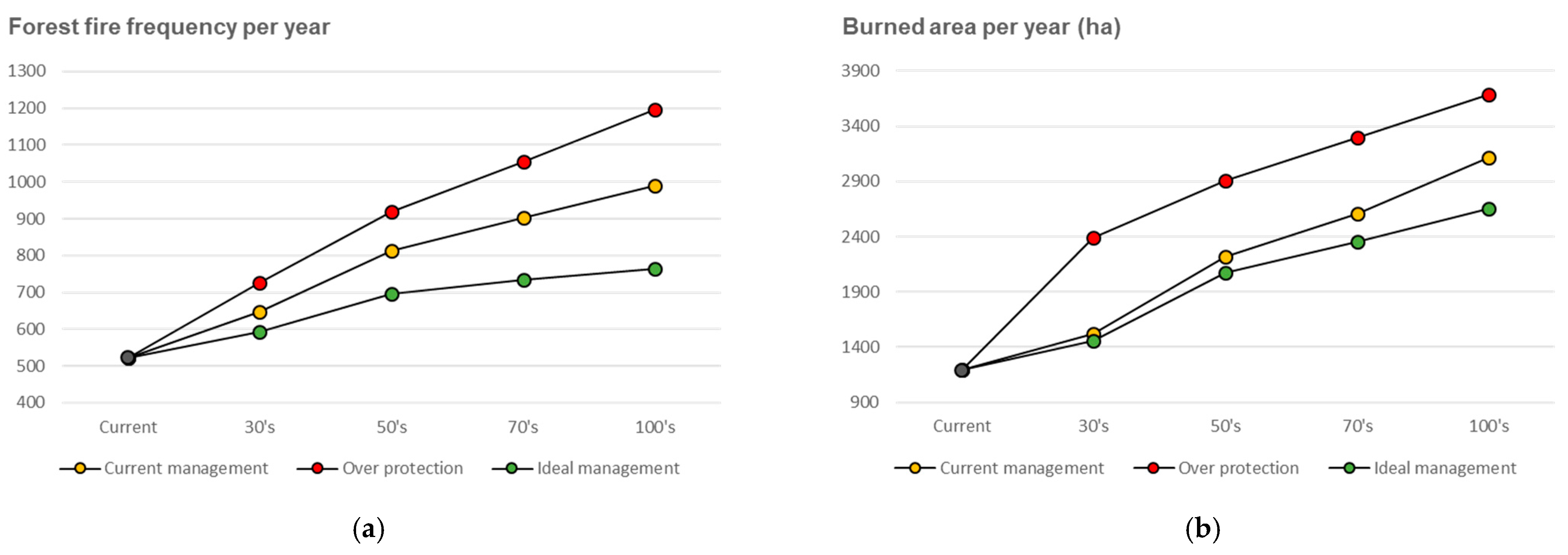
4.4. Simulation of the Future Forest Fire Events

As a result of the optimization, FLAM can be used to project the patterns of forest fires into the future by exploiting diverse scenario datasets, which can provide useful insights for developing adaptation strategies for reducing the risk of forest fires. Therefore, we further examined its applicability for future projections by using the forest management scenario produced by Hong [26]. According to the projection illustrated in Figure 16, both the forest fire frequency and burned area are expected to increase due to the increasing amount of fuel in all three future scenarios: maintaining the current management, over protection, and applying the ideal management plan based on the sixth basic forest plan of South Korea [44]. Nevertheless, applying the ideal forest management plan, which actively harvests wood products from over-matured forests, could decrease the forest fire frequency to 63–81% of the over protection scenario and to 77–92% of current management. The burned area could be decreased to 61–72% of the over protection scenario and to 85–96% of current management.

5. Discussion

In this study, probability algorithms in FLAM developed for a global application were optimized and downscaled to the environment of South Korea to project forest fires at a local scale. The optimization was performed by using a dataset from January 2016 to March 2022, most of which were collected from domestic sources and aimed at adjusting the key parameters for interpreting human and biophysical impacts on forest fires. These includes parameters such as population density, lightning frequency, fuel moisture, and the amount of fuel. Previous studies on FLAM focused on modeling the burned area. Because of the limitations introduced by using global datasets, which often lack fire frequency information, this study provided a deeper look at forest fire frequency. Fire frequency is important for interpreting forest fire ignition patterns and as an intermediate process for the further improvement of burned area projections. The simulation results showed that the modeling of the forest fire frequency was considerably improved by the optimization from the sub-optimal evaluation score with a correlation coefficient r of 0.050 and 0.447 to a correlation coefficient r of over 0.89 when tested for two different time periods. The simulation of the burned area performed without the optimization of the fire spread algorithm showed a reliable correlation only for small-scale fires, which is proportional to forest fire frequency.

As the optimization process included adjusting substantial amounts of parameters for interpreting various factors, downscaling, and introducing new equations, the best optimization options were selected step by step with a trial-and-error method aimed at reproducing historical forest fire patterns. In this context, C_calib is one of the most important factors in the current optimization process to offset the impact of accumulated error at each optimization step, but at the same time it represents the limitation of the current optimization process. Even though the process could handle the multiple optimization tasks efficiently and suggested overall optimization frameworks supported by background studies, a further improvement of each equation is recommended to develop more effective equation forms based on the statistical analysis of forest fire patterns. For example, the ignition probability by human sources needs to be improved to interpret the dispersion of human activity so that the downscaled application of FLAM could reproduce large-scale hotspots near cities. Ignitions from technical faults, such as embers generated from power lines, also need to be considered.

In addition, the current FLAM framework includes limitations on reflecting forest fire dynamics with multiple spatial contexts as it was designed to calculate forest fire probabilities on a given scale. It indicates that downscaling the algorithm with the framework has a risk of losing accuracy when the scale is too small to capture significant environmental factors of a forest fire. Therefore, the modelling framework needs to be improved, especially for downscaling purposes, so it can incorporate a cross-scale interaction that occurs in natural phenomena [45].

Although the optimization process can be further improved, the results of the optimized FLAM were promising and especially interesting because they demonstrated the agreement between probability P_m conditional on the fuel moisture content and time series patterns of forest fire frequency in South Korea (Figure 11). These results show the importance of P_m on projecting forest fire frequency and can be interpreted as evidence of the successful optimization of the FFMC algorithm. In addition, the underlying hypothesis of the FFMC optimization was that the rate of soil moisture change becomes more highly proportional to Fr. This hypothesis is in line with the literature that both soil moisture changes and evapotranspiration from soil were faster in forests compared to grasslands [46,47] and that the topsoil moisture content was more varied over time when the grass coverage was higher [48].

This study found that the P_m in the spring season over the observed 7 years was significantly increasing in the east coastal area, which is already prone to frequent and severe forest fires. The findings suggest that the risk of forest fires is increasing due to climate change, which has important implications for forest fire management and adaptation strategies in South Korea. With the risk of forest fires increasing in certain regions, it is essential to develop and implement effective forest fire prevention and suppression measures. This may include increasing the availability of firefighting resources, improving the early warning systems, and implementing land management practices that can reduce the risk of ignition, such as fuel reduction with a proper forest management plan. In addition, it is important to continue to monitor P_m and other environmental factors that affect the risk of forest fires to identify areas that are particularly susceptible to future fires. Experiments on the optimized FLAM, downscaled to 1 km² in this study, with the latest environmental observations can be used to develop adaptation strategies that are tailored to the specific risks and challenges faced by different regions.

6. Conclusions

In this study, we optimized FLAM to the environment of South Korea based on the national GIS data downscaled to a 1 km² resolution with additional algorithms introduced for reproducing the national specific patterns of forest fire frequency, such as ignition from agricultural waste burning. For the forest fire frequency aggregated over South Korea, we obtained Pearson’s correlation coefficient r of 0.893 for a temporal evaluation and 0.802 for a spatial evaluation. This showed that the optimized FLAM is capable of capturing both spatial and temporal patterns of forest fire frequency with a valid reproduction of historical forest fire patterns. Considering that the pre-optimization algorithms produced sub-optimal results with an r of 0.171, FLAM is applicable to South Korea only after the optimization of all its modules. Its main algorithms for interpreting biophysical and human impacts on forest fires on a global scale were insufficient without the optimization. Moreover, this study overcame a limitation of previous studies on FLAM: an inability to examine more closely forest fire frequency because of the limited availability of data, i.e., using large-scale datasets. This makes the optimization performed in this study valuable for the model development and its applications to other regions of the world.

The algorithm for the FFMC was improved by fitting the moisture content m to remotely sensed soil moisture to incorporate land surface environment in FLAM for a better representation of local fuel moisture variations linked to vegetation. With the improved algorithms for South Korea, a time-series pattern of probability P_m conditional on the moisture content showed a good agreement with the seasonal patterns of forest fire frequency. Meanwhile, based on the simulated forest fire frequency, a dense population in an urbanized area in combination with other factors was shown to lead to an exponentially increasing probability of fire. In this context, P_m seems to be the most plausible factor for exploding forest fires in the future, as the increasing trend of P_m adds an additional threat to the already affected areas, which can be interpreted as a result of a changing climate.

Because the optimization succeeded to reproduce the national specific pattern of forest fires in South Korea, it should be followed by research into developing adaptation strategies for reducing forest fire risks with a diverse application of the future scenarios’ dataset. This study has already presented a future projection by using forest management scenarios and showed the effect of ideal forest management, reducing approximately a quarter of forest fire frequency. Therefore, the next task aims to undercover the best adaptation scenario by integrating climate change scenario datasets with multiple adaptation options in consideration of feasibility, cost effectiveness, regional priority, etc.

In this context, the FLAM iteration that currently works with probabilities could be modified to an agent-based model (ABM) to better identify the tipping point or threshold that provokes extreme forest fire events. For example, if the fire spread algorithm of FLAM is converted to an ABM and reflects the limited suppression capability in the algorithms, the burned areas caused by large-scale forest fires can be better estimated as unsuppressed fire spreading between adjacent pixels and modeled by the interactions between agents. Conversely, ideal suppression capabilities minimize forest fire damage, or at least do not surpass the threshold leading to extreme fires, in various climate change scenarios.

Optimizations improved the overall accuracy of FLAM in the context of South Korea through the inclusion of regional drivers and variability, which reflect the role of climate and human actions in the occurrence of wildfire events. The presented results are a starting point for modeling a future burned area under various climate change scenarios. They highlight the need and efficacy of intensive forest fire management to mitigate the growing risk and reduce the probability of extreme wildfire events in Korea under a changing climate.

References

1. Sutanto, S.J.; Vitolo, C.; Di Napoli, C.; D’Andrea, M.; Van Lanen, H.A. Heatwaves, droughts, and fires: Exploring compound and cascading dry hazards at the pan-European scale. Environ. Int. 2020, 134, 105276. [Google Scholar] [CrossRef] [PubMed]
2. Clark, J.S.; Royall, P.D.; Chumbley, C. The role of fire during climate change in an eastern deciduous forest at Devil’s Bathtub, New York. Ecology 1996, 77, 2148–2166. [Google Scholar] [CrossRef]
3. Randerson, J.T.; Liu, H.; Flanner, M.G.; Chambers, S.D.; Jin, Y.; Hess, P.G.; Pfister, G.; Mack, M.C.; Treseder, K.K.; Welp, L.R.; et al. The impact of boreal forest fire on climate warming. Science 2006, 314, 1130–1132. [Google Scholar] [CrossRef] [Green Version]
4. Lim, C.H.; Kim, Y.S.; Won, M.; Kim, S.J.; Lee, W.K. Can satellite-based data substitute for surveyed data to predict the spatial probability of forest fire? A geostatistical approach to forest fire in the Republic of Korea. Geomat. Nat. Hazards Risk 2019, 10, 719–739. [Google Scholar] [CrossRef] [Green Version]
5. Munang, R.; Thiaw, I.; Alverson, K.; Liu, J.; Han, Z. The role of ecosystem services in climate change adaptation and disaster risk reduction. Curr. Opin. Environ. Sustain. 2013, 5, 47–52. [Google Scholar] [CrossRef]
6. Varela, V.; Vlachogiannis, D.; Sfetsos, A.; Karozis, S.; Politi, N.; Giroud, F. Projection of Forest Fire Danger due to Climate Change in the French Mediterranean Region. Sustainability 2019, 11, 4284. [Google Scholar] [CrossRef] [Green Version]
7. Jadmiko, S.D.; Murdiyarso, D.; Faqih, A. Climate changes projection for land and forest fire risk assessment in West Kalimantan. IOP Conf. Ser. Earth Environ. Sci. 2017, 58, 012030. [Google Scholar] [CrossRef] [Green Version]
8. Wang, S.W.; Kim, W.; Song, C.; Park, E.; Jo, H.W.; Kim, J.; Lee, W.K. Relationships among water, food, energy, and ecosystems in the Mid-Latitude Region in the context of sustainable development goals. Environ. Rev. 2022, accepted. [Google Scholar] [CrossRef]
9. Song, C.; Pietsch, S.A.; Kim, M.; Cha, S.; Park, E.; Shvidenko, A.; Schepaschenko, D.; Kraxner, F.; Lee, W.K. Assessing forest ecosystems across the vertical edge of the mid-latitude ecotone using the biogeochemistry management model (BGC-MAN). Forests 2019, 10, 523. [Google Scholar] [CrossRef] [Green Version]
10. Moritz, M.A.; Batllori, E.; Bradstock, R.A.; Gill, A.M.; Handmer, J.; Hessburg, P.F.; Leonard, J.; McCaffrey, S.; Odion, D.C.; Schoennagel, T.; et al. Learning to coexist with wildfire. Nature 2014, 515, 58–66. [Google Scholar] [CrossRef] [PubMed]
11. Engle, N.L.; de Bremond, A.; Malone, E.L.; Moss, R.H. Towards a resilience indicator framework for making climate-change adaptation decisions. Mitig. Adapt. Strateg. Glob. Chang. 2014, 19, 1295–1312. [Google Scholar] [CrossRef]
12. Korea Forest Service. Forest Fire Risk Prediction System. Available online: https://forest.go.kr/newkfsweb/html/HtmlPage.do?pg=/fgis/UI_KFS_5002_030203.html&orgId=fgis&mn=KFS_02_04_03_05_02 (accessed on 12 December 2022).
13. Sung, M.K.; Lim, G.H.; Choi, E.H.; Lee, Y.Y.; Won, M.S.; Koo, K.S. Climate change over Korea and its relation to the forest fire occurrence. Atmosphere 2010, 20, 27–35. [Google Scholar]
14. Won, M.; Yoon, S.; Jang, K. Developing Korean forest fire occurrence probability model reflecting climate change in the spring of 2000s. Korean J. Agric. For. Meteorol. 2016, 18, 199–207. [Google Scholar] [CrossRef] [Green Version]
15. Arora, V.K.; Boer, G.J. Fire as an interactive component of dynamic vegetation models. J. Geophys. Res. Biogeosci. 2005, 110, G02008. [Google Scholar] [CrossRef] [Green Version]
16. Kloster, S.; Mahowald, N.M.; Randerson, J.T.; Thornton, P.E.; Hoffman, F.M.; Levis, S.; Lawrence, P.J.; Feddema, J.J.; Oleson, K.W.; Lawrence, D.M. Fire dynamics during the 20th century simulated by the Community Land Model. Biogeosciences 2010, 7, 1877–1902. [Google Scholar] [CrossRef] [Green Version]
17. Gavin, D.G.; Hallett, D.J.; Hu, F.S.; Lertzman, K.P.; Prichard, S.J.; Brown, K.J.; Lynch, J.A.; Bartlein, P.; Peterson, D.L. Forest fire and climate change in western North America: Insights from sediment charcoal records. Front. Ecol. Environ. 2007, 5, 499–506. [Google Scholar] [CrossRef]
18. Fernandez-Anez, N.; Krasovskiy, A.; Müller, M.; Vacik, H.; Baetens, J.; Hukić, E.; Kapovic Solomun, M.; Atanassova, I.; Glushkova, M.; Bogunović, I.; et al. Current wildland fire patterns and challenges in Europe: A synthesis of national perspectives. Air Soil Water Res. 2021, 14, 11786221211028185. [Google Scholar] [CrossRef]
19. Cimdins, R.; Krasovskiy, A.; Kraxner, F. Regional Variability and Driving Forces behind Forest Fires in Sweden. Remote Sens. 2022, 14, 5826. [Google Scholar] [CrossRef]
20. Migliavacca, M.; Dosio, A.; Kloster, S.; Ward, D.S.; Camia, A.; Houborg, R.; Houston Durrant, T.; Khabarov, N.; Krasovskii, A.A.; San Miguel-Ayanz, J.; et al. Modeling burned area in Europe with the Community Land Model. J. Geophys. Res. Biogeosci. 2013, 118, 265–279. [Google Scholar] [CrossRef] [Green Version]
21. Khabarov, N.; Krasovskii, A.; Obersteiner, M.; Swart, R.; Dosio, A.; San-Miguel-Ayanz, J.; Durrant, T.; Camia, A.; Migliavacca, M. Forest fires and adaptation options in Europe. Reg. Environ. Chang. 2016, 16, 21–30. [Google Scholar] [CrossRef] [Green Version]
22. Krasovskii, A.; Khabarov, N.; Pirker, J.; Kraxner, F.; Yowargana, P.; Schepaschenko, D.; Obersteiner, M. Modeling burned areas in Indonesia: The FLAM approach. Forests 2018, 9, 437. [Google Scholar] [CrossRef] [Green Version]
23. Park, E.; Jo, H.W.; Lee, W.K.; Lee, S.; Song, C.; Lee, H.; Park, S.; Kim, W.; Kim, T.H. Development of earth observational diagnostic drought prediction model for regional error calibration: A case study on agricultural drought in Kyrgyzstan. GIsci. Remote Sens. 2022, 59, 36–53. [Google Scholar] [CrossRef]
24. Korea Forest Service. Yearbook of Forest Fire Statistics; Association Together with the Disabled: Seoul, Republic of Korea, 2022. Available online: https://www.forest.go.kr/kfsweb/cmm/fms/FileDown.do?atchFileId=FILE_000000020067170&fileSn=1&dwldHistYn=Y&bbsId=BBSMSTR_1008 (accessed on 25 January 2023).
25. Lee, J.G.; In, S.R. A numerical sensitivity experiment of the downslope windstorm over the Yeongdong region in relation to the inversion layer of temperature. Atmosphere 2009, 19, 331–344. [Google Scholar]
26. Hong, M.; Song, C.; Kim, M.; Kim, J.; Lee, S.G.; Lim, C.H.; Cho, K.; Son, Y.; Lee, W.K. Application of integrated Korean forest growth dynamics model to meet NDC target by considering forest management scenarios and budget. Carbon Balance Manag. 2022, 17, 1–18. [Google Scholar] [CrossRef] [PubMed]
27. Lee, S.J.; Yim, J.S.; Son, Y.M.; Son, Y.; Kim, R. Estimation of forest carbon stocks for national greenhouse gas inventory reporting in South Korea. Forests 2018, 9, 625. [Google Scholar] [CrossRef] [Green Version]
28. Park, E. Assessment of Afforestation Options with Special Emphasis on Forest Productivity and Carbon Storage in North Korea. 2021. Available online: https://pure.iiasa.ac.at/id/eprint/17471/ (accessed on 25 January 2023).
29. Richards, F.J. A flexible growth function for empirical use. J. Exp. Bot. 1959, 10, 290–301. [Google Scholar] [CrossRef]
30. Chen, J.; Jönsson, P.; Tamura, M.; Gu, Z.; Matsushita, B.; Eklundh, L. A simple method for reconstructing a high-quality NDVI time-series data set based on the Savitzky–Golay filter. Remote Sens. Environ. 2004, 91, 332–344. [Google Scholar] [CrossRef]
31. Van Wagner, C.E.; Pickett, T.L. Equations and Fortran Program for the Canadian Forest Fire Weather Index System; Canadian Forestry Service: Ottawa, ON, Canada, 1985; Volume 33.
32. Krasovskii, A.; Khabarov, N.; Migliavacca, M.; Kraxner, F.; Obersteiner, M. Regional aspects of modelling burned areas in Europe. Int. J. Wildland Fire 2016, 25, 811–818. [Google Scholar] [CrossRef] [Green Version]
33. Bergeron, Y.; Flannigan, M.; Gauthier, S.; Leduc, A.; Lefort, P. Past, current and future fire frequency in the Canadian boreal forest: Implications for sustainable forest management. AMBIO J. Hum. Environ. 2004, 33, 356–360. [Google Scholar] [CrossRef] [PubMed]
34. Kim, S.J.; Lim, C.H.; Kim, G.S.; Lee, J.; Geiger, T.; Rahmati, O.; Son, Y.; Lee, W.K. Multi-temporal analysis of forest fire probability using socio-economic and environmental variables. Remote Sens. 2019, 11, 86. [Google Scholar] [CrossRef] [Green Version]
35. Ganteaume, A.; Camia, A.; Jappiot, M.; San-Miguel-Ayanz, J.; Long-Fournel, M.; Lampin, C. A review of the main driving factors of forest fire ignition over Europe. Environ. Manag. 2013, 51, 651–662. [Google Scholar] [CrossRef] [PubMed] [Green Version]
36. Kim, J.H.; Lee, H.J. Study on Cases of Priority Traffic Signal System for Emergency Vehicles: Based on a City’s Pilot Operation Cases in Chungcheongbukdo Province. Fire Sci. Eng. 2020, 34, 121–126. [Google Scholar] [CrossRef] [Green Version]
37. Scandella, F. Firefighters: Feeling the Heat; European Trade Union Institute: Brussels, Belgium, 2012. [Google Scholar]
38. Lawson, B.D.; Armitage, O.B. Weather Guide for the Canadian Forest Fire Danger Rating System; Canadian Forest Service: Edmonton, AB, Canada, 2008.
39. Wang, P.X.; Li, X.W.; Gong, J.Y.; Song, C. Vegetation temperature condition index and its application for drought monitoring. In Proceedings of the IGARSS 2001. Scanning the Present and Resolving the Future. Proceedings. IEEE 2001 International Geoscience and Remote Sensing Symposium, Sydney, NSW, Australia, 9–13 July 2001; Volume 1, pp. 141–143. [Google Scholar]
40. Patel, N.R.; Mukund, A.; Parida, B.R. Satellite-derived vegetation temperature condition index to infer root zone soil moisture in semi-arid province of Rajasthan, India. Geocarto Int. 2022, 37, 179–195. [Google Scholar] [CrossRef]
41. Sun, H. Two-stage trapezoid: A new interpretation of the land surface temperature and fractional vegetation coverage space. IEEE J. Sel. Top. Appl. Earth Obs. Remote Sens. 2015, 9, 336–346. [Google Scholar] [CrossRef]
42. Lee, S.Y.; An, S.H.; Won, M.S.; Lee, M.B.; Lim, T.G.; Shin, Y.C. Classification of forest fire occurrence risk regions using GIS. J. Korean Assoc. Geogr. Inf. Studies 2004, 7, 37–46. [Google Scholar]
43. Gillies, R.R.; Kustas, W.P.; Humes, K.S. A verification of the ‘triangle’ method for obtaining surface soil water content and energy fluxes from remote measurements of the Normalized Difference Vegetation Index (NDVI) and surface e. Int. J. Remote Sens. 1997, 18, 3145–3166. [Google Scholar] [CrossRef]
44. Korea Forest Service. The 6th Basic Forest Plan (2018~2037); Korea Forest Service: Daejeon, Republic of Korea, 2018; p. 151.
45. Turner, M.G.; Gardner, R.H. Introduction to landscape ecology and scale. In Landscape Ecology in Theory and Practice: Pattern and Process; Springer: New York, NY, USA, 2015; pp. 1–32. [Google Scholar]
46. Pérez-Corona, M.E.; Pérez-Hernández, M.D.C.; Medina-Villar, S.; Andivia, E.; Bermúdez de Castro, F. Canopy species composition drives seasonal soil characteristics in a Mediterranean riparian forest. Eur. J. For. Res. 2021, 140, 1081–1093. [Google Scholar] [CrossRef]
47. Rahgozar, M.; Shah, N.; Ross, M. Estimation of evapotranspiration and water budget components using concurrent soil moisture and water table monitoring. Int. Sch. Res. Notices 2012, 2012, 726806. [Google Scholar] [CrossRef] [Green Version]
48. Yang, W.; Wang, Y.; He, C.; Tan, X.; Han, Z. Soil water content and temperature dynamics under grassland degradation: A multi-depth continuous measurement from the agricultural pastoral ecotone in Northwest China. Sustainability 2019, 11, 4188. [Google Scholar] [CrossRef] [Green Version]
Figure 1. Patterns of the forest fires frequency and their scale in South Korea (from January 2016 to March 2022).
Remotesensing 15 01446 g001
Figure 2. Architecture of the FLAM model. The indicated sections correspond to the section of the paper where each part of the model is explained: Section 3.2 for ignition probability, Section 3.3 for fuel moisture content calculation, and Section 3.4 for probability of fire. Each component of the flowchart is colored according to its improvement from the original FLAM, as indicated by the legend at the bottom right.
Remotesensing 15 01446 g002
Figure 3. Conceptual illustration of potential overestimations of fire caused by the monthly lightning frequency and daily weather.
Remotesensing 15 01446 g003
Figure 4. Number and ratio of forest fires ignited from (agricultural) waste burning.
Remotesensing 15 01446 g004
Figure 5. Number of forest boundary grids neighboring the agricultural field.
Remotesensing 15 01446 g005
Figure 6. Concept of Vegetation Temperature Condition Index (VTCI) in the LST-NDVI feature space.
Remotesensing 15 01446 g006
Figure 7. Optimization of the ignition probability by human factors: (a) original probabilities at global scale, (b) optimized probabilities for South Korea.
Remotesensing 15 01446 g007
Figure 8. Optimization of the ignition probability conditional on lightning frequency: (a) original probabilities at a global scale, (b) optimized probabilities for South Korea, (c) probability distribution calculated with monthly dataset and the original parameters, (d) probability distribution calculated with daily dataset and the optimized parameters.
Remotesensing 15 01446 g008
Figure 9. Comparison of daily fuel moisture increment calculated by FFMC and VTCI.
Remotesensing 15 01446 g009
Figure 10. Fuel moisture difference between FFMC and VTCI in ∆m—fractional vegetation cover data space.
Remotesensing 15 01446 g010
Figure 11. Temporal evaluation of forest fire frequency simulated by the optimized FLAM.
Remotesensing 15 01446 g011
Figure 12. Temporal evaluation of burned area simulated by the optimized FLAM.
Remotesensing 15 01446 g012
Figure 13. Spatial evaluation of forest fire frequency simulated by the optimized FLAM: (a) period A from January 2016 to December 2019, (b) period B from January 2020 to March 2022.
Remotesensing 15 01446 g013
Figure 14. Expected number of forest fires throughout the study period: (a) simulation of the optimized FLAM, (b) observation.
Remotesensing 15 01446 g014
Figure 15. Trends of the ignition probability conditional on fuel moisture (Pm) in spring season: (a) average Pm, (b) slope of the time-series Pm, (c) Pearson’s correlation coefficient of the time series Pm.
Remotesensing 15 01446 g015
Figure 16. Future projection of forest fires by the optimized FLAM based for the forest management scenario [26]: (a) forest fire frequency per year, (b) burned area per year.
Remotesensing 15 01446 g016