Article

Irrigation Timing Retrieval at the Plot Scale Using Surface Soil Moisture Derived from Sentinel Time Series in Europe

1
CESBIO, Université de Toulouse, CNRS/UPS/IRD/CNES/INRAE, 18 Avenue Edouard Belin, Bpi 2801, 31401 Toulouse, France
2
CNRM-Météo-France/CNRS, Université de Toulouse, 42 ave G. Coriolis, 31075 Toulouse, France
3
Department of Civil and Environmental Engineering, University of Perugia, Via G. Duranti, 93, 06125 Perugia, Italy
4
Research Institute for Geo-Hydrological Protection, National Research Council, Via Madonna Alta 126, 06128 Perugia, Italy
5
Climate and Environmental Remote Sensing (CLIMERS) Research Group, Department of Geodesy and Geoinformation, TU Wien, 1040 Vienna, Austria
*
Author to whom correspondence should be addressed.
Remote Sens. 2023, 15(5), 1449; https://doi.org/10.3390/rs15051449
Submission received: 22 December 2022 / Revised: 23 February 2023 / Accepted: 28 February 2023 / Published: 4 March 2023
(This article belongs to the Special Issue Irrigation Estimates and Management from EO Data)

Abstract

:
The difficulty of calculating the daily water budget of irrigated fields is often due to the uncertainty surrounding irrigation amounts and timing. The automated detection of irrigation events has the potential to greatly simplify this process, and the combination of high-resolution SAR (Sentinel-1) and optical satellite observations (Sentinel-2) makes the detection of irrigation events feasible through the use of a surface soil moisture (SSM) product. The motivation behind this study is to utilize a large irrigation dataset (collected during the ESA Irrigation + project over five sites in three countries over three years) to analyze the performance of an established algorithm and to test potential improvements. The study’s main findings are (1) the scores decrease with SSM observation frequency; (2) scores decrease as irrigation frequency increases, which was supported by better scores in France (more sprinkler irrigation) than in Germany (more localized irrigation); (3) replacing the original SSM model with the force-restore model resulted in an improvement of about 6% in the F-score and narrowed the error on cumulative seasonal irrigation; (4) the Sentinel-1 configuration (incidence angle, trajectory) did not show a significant impact on the retrieval of irrigation, which supposes that the SSM is not affected by these changes. Other aspects did not allow a definitive conclusion on the irrigation retrieval algorithm: (1) the lower scores obtained with small NDVI compared to large NDVI were counter-intuitive but may have been due to the larger number of irrigation events during high vegetation periods; (2) merging different runs and interpolating all SSM data for one run produced comparable F-scores, but the estimated cumulative sum of irrigation was around −20% lower compared to the reference dataset in the best cases.

1. Introduction

Irrigation water use is a critical factor in managing and optimizing agricultural water resources amid the increasing global demand for irrigation water [1]. The rise in demand is particularly noticeable in response to the production of bioenergy [2], while the decrease in groundwater availability amplifies competition with other sectors, including urban water demand [3]. An irrigation, like a precipitation event, has a specific start and end time, during which a given amount of water is applied to the field, usually referred to as the amount or dose of irrigation. This quantity is expressed either as a volume (m3) or a water depth (mm) at the field (plot) level. Quantifying irrigation has been mainly carried out at large scales using a method based on coarse-scale surface soil moisture products derived from either passive or active remote sensing sensors [4,5,6,7]. These techniques operate in the microwave domain where the dielectric properties of soil are primarily governed by its water content, which directly affects the emissivity and backscattering of the soil surface [8]. However, such methods operate at much lower resolutions than the field scale, and detecting irrigation events at the field scale is an emerging scientific area.
Land surface temperature provides an attractive proxy of root-zone soil moisture conditions as hydrologically stressed vegetation heats up in response to stomatal closure [9]. Olivera-Guerra et al. [10] derived crop water stress from Landsat land surface temperature data to feed a simple crop balance model for estimating irrigation water timing and amount. However, this method faces limitations, mainly attributed to the low revisit time of available thermal sensors into orbit. Nevertheless, this method is promising in the short term with the launch of new thermal sensors such as TRISHNA (Thermal InfraRed Imaging Satellite for High-resolution Natural resource Assessment, https://www.eoportal.org/satellite-missions/trishna, accessed the 2 February 2023) expected for 2024 or LSTM (Land Surface Temperature Monitoring, https://www.eoportal.org/satellite-missions/lstm accessed the 2 February 2023), expected for 2028.
In addition to the work mentioned above, most of the approaches developed recently rely on surface soil moisture (SSM) estimates derived from Sentinel-1. The dielectric properties of the soil phases (i.e., water, air, and solids) affect the emissivity and backscattering of microwaves from the soil surface [8], making it possible to retrieve soil moisture from microwave observations. The Sentinel-1 C-band satellites have penetration ranges from 1.87 to 3.75 cm and 0.75 to 1.5 cm for bare soil and cultivated soil, respectively, making it theoretically possible to estimate SSM at the nominal resolution of Sentinel-1 of 10 m. However, to decrease the well-known noise of radar observations due to interference from the coherent sum of scattered signals, also called “speckle noise,” the results are generally provided at a lower resolution.
Bazzi et al. [11] took advantage of the difference in footprint between rainfall that waters a large area (>1 km) and an irrigation event whose impact is limited to the field by comparing the dynamic of the radar signal at both scales. This work has been updated [12] with a new study over summer crops, where the main findings indicated that the density of available Sentinel-1 affects the irrigation detection accuracy, especially for temperate areas. Le Page et al. [13] compared the relative change of surface soil moisture predicted by a simple soil water budget model, with no representation of irrigation and derived from Sentinel-1 [14], on maize plots to determine the timing of irrigation events. Ouaadi et al. [15] proposed an approach based on the assimilation of high-resolution soil moisture products [16] into a simple soil water budget model and demonstrated that both irrigation timing and water amounts could be retrieved with reasonable accuracy if the irrigation techniques (flooding or drip irrigation) were known. A recent study of Zappa et al. [4] analyzed the accuracy of irrigation retrieval from space as a function of the characteristics of soil moisture products, and indirectly the irrigation techniques demonstrated that (1) improved metrics are obtained with high spatial and temporal resolution products; (2) better results are obtained on fields where large amounts of water are applied such as for a traditional flooding irrigation method. Brombacher et al. [17] have proposed an alternative approach based on the comparison of evapotranspiration of natural areas to the evapotranspiration of irrigated fields. The difference of evapotranspiration is attributed to irrigation water amounts.
The detection of irrigation events in [13] relied on a relative comparison between two assessments of SSM. The first assessment was obtained from satellite observations, while the second assessment was obtained from a water budget model based on the FAO-56 model [18]. The comparison between the two assessments was conducted at each satellite observation. The method of irrigation timing retrieval was developed and tested on a small dataset of six maize plots over one season in southwest France. Consequently, the examination of the model’s performance did not permit a detailed analysis of its effectiveness. The ESA Irrigation+ project dataset, which provides a wide variety of crops, soils, and irrigation methods in different European countries, is much larger and thus used to evaluate the method with respect to crop type and irrigation method. This study aims at evaluating this method according to the kind of crop, and the type of irrigation. We also have organized the study in order to analyze impact of the configuration of the Sentinel-1 acquisitions (incidence angle, and orbit), and two classes of vegetation development by separating between small NDVI and high NDVI.
In addition to these evaluations, the force-restore approach [19] is tested as an alternative to the original bucket model in order to estimate SSM. Finally, two different strategies for using the observations of SSM are also tested.
The article is organized into four parts. The first part describes the study area and analyzes the forcing and validation datasets. The ESA Irrigation+ dataset is examined to demonstrate the diversity of crops, soils, irrigation methods, and schedules. The weather data, Sentinel-2 NDVI, and Sentinel-1 SSM datasets are then described. The second part outlines the methodology, briefly describing the model and providing the model equations in different annexes (Appendix A). Additionally, the statistics used are described. The third part presents the results, and the final part discusses conclusions and future works.

2. Dataset and Irrigation Detection Approach

The irrigation detection method relies on a simple water budget based on the FAO-56 model [20] that is forced by precipitation, the reference evapotranspiration ET0, the basal crop coefficient Kcb, the fractional cover derived from Sentinel-2 NDVI at a daily time step [21], and satellite-derived products of surface soil moisture. The performance of the approach is assessed over different plots in Europe described in the following section. A short description of the methodology is provided afterward, and the system of equations is fully described in Appendix A.2 and Appendix A.3.

2.1. Study Sites and Irrigation Data

The large dataset consists of a time series of irrigation events characterized by their timing and water amount for different plots in Europe (Figure 1) The data were gathered in five different regions: Niedersachsen and Brandenburg in Germany, Lot and Tarn in France, and Budrio in Italy, within the frame of the ESA Irrigation+ project [5]. According to the Koppen–Geiger climate classification, Niedersachsen, Lot and Tarn are located in a temperate oceanic climate (Cfb); Brandenburg is located in a humid continental climate (Dfb); and Budrio in a humid subtropical climate (Cfa). There are 85 different plots with data acquired over three seasons from September 2017 to September 2019 depending on the plot for a total of 105 complete growing seasons (see Appendix A.5 for details). The size of the plots ranges from 0.3 to 10 ha. The soil texture has been retrieved from the OpenLandMap dataset using Google Earth Engine (GEE), a dataset based on machine learning predictions from a global compilation of soil profiles and samples. It is an enhancement of SoilGrids from Hengl et al. [22]. Tarn and Lot have clay loam soils (~30% clay and ~30% sand); Budrio has silty clay loam soils. The two German regions have more sandy textures: sandy loam for Brandenburg and loam for Niedersachsen [23] (Figure 1). Table 1 describes the number of available plots/seasons by region and crop type. Most of the crops are cereals, consisting of maize, rye, wheat, and barley. The second most important crops in the dataset are tubers (potato and sugar beet). There are also some vegetables (mainly soybean), and crops used for fodder (maize, rapeseed, grass). Plots seeded with walnut and tobacco complete the dataset. However, as full descriptions (eg. Kcb, Fc, rooting depth) of some of those crops were unknown, they were given the configuration of a similar crop (for example, wheat for barley or maize for rye).
The irrigation characteristics of the five study areas are shown in Figure 2 in terms of amount, number per year, and frequency. Note that the amount of water per event is not known for Brandenburg, and was set at 15 mm/event. The average number of irrigation events per season is between 7 and 9 for the regions of Brandenburg, Tarn, and Lot, where sprinkler irrigation dominates. Budrio, with an average of 18 events per season, has a mix of sprinkler and drip irrigation. On average, Niedersachsen has a high number of irrigation events (24 on average, 80 maximum) with an average amount of 18 mm, but with a big variation of the amount between fields. As such, this area is dominated with drip irrigation but also has sprinkler irrigated fields.
Le Page et al. [13] showed that low amounts (less than 10 mm per event) make irrigation detection difficult. In this dataset, only a few events, located mainly in Niedersachsen and Budrio, are below this threshold. Likewise, the detection was also shown to be difficult if the frequency of irrigation is higher than the time of the satellite overpass (6 days for the combination of Sentinel-1A and Sentinel-1B), such as in the Niedersachsen region where the average irrigation frequency is 2.8 days.
Figure 3 shows the distribution over time of the irrigation season per region, while Figure 4 presents the season of irrigation for the main crop types. The season duration can extend for as long as 150 days in Brandenburg and be as short as one day at the French locations (one irrigation event only). The irrigation season begins around mid-April and ends around mid-September on average, except for in France where the irrigation season is very short (from June to mid-September) because maize, irrigated during the summer months, is the dominant crop in this region. Regarding the irrigation season of the main crops investigated in this study, wheat is generally irrigated from May to June, potato from May to August, and tomato from May to September.

2.2. Weather Data

The weather data needed to compute the water budget are the daily precipitation and reference evapotranspiration. When available, the rainfall measured by rain gauges is located close to the plot (Germany and Italy). In France, those measurements were not available outside of the irrigation season. For the latter or in the case of missing data, the amounts were provided by the AgERA5 dataset [24], at a spatial resolution of 0.1° × 0.1°. Likewise, while the FAO-56 water budget approach relies on the reference evapotranspiration (ET0, Allen et al. [20]), the potential evapotranspiration (PET) relying on MODIS (MODerate resolution Imaging Spectroradiometer) observations was used for ease of implementation. PET rates from the 8-day aggregated MOD16A2 product at 500 m spatial resolution were extracted through the GEE platform.

2.3. Vegetation INDEX, LAND COVER, and Crop Season

NDVI and Land cover are needed to estimate the basal crop coefficient Kcb for each crop and plot. Time series of NDVI from the Sentinel-2A and 2B satellites were retrieved and averaged over the plot using the COPERNICUS/S2_SR collection from GEE. This dataset is atmospherically corrected with the Sen2cor algorithm [25]. Although other algorithms can perform better [26], this processing provides a coherent time series of surface reflectance. The time series were further cloud-masked using the COPERNICUS/S2_CLOUD_PROBABILITY collection, which is a GEE precomputed dataset obtained with the s2cloudless algorithm. An automated cloud-detection algorithm is based on a gradient boosting algorithm which is fast and performs well [27]. As some clouds might still persist in the time series, the well-known Savitsky–Golay filter [28] has been applied in order to smooth the times series of NDVI. Figure 5 displays an example of NDVI time series before and after smoothing. The seasonal land cover type used for the relations between NDVI and fractional vegetation cover, and with NDVI and basal crop coefficient, was retrieved directly from the different dataset providers. The duration of the crop season was determined by an ad hoc peak and valley algorithm. The algorithm searches for local minimums and maximums on the smoothed time series of NDVI, and it deletes consecutive minimums or maximums. It then selects the local maximums above 0.6, and only keeps them if there is a duration of at least 90 days between two local maximums. The beginning and end of each season are found as the local minimums in the time series before and after each selected local maximum. An example result is given in Figure 5.

2.4. Surface Soil Moisture “S2SM” Dataset

The S2SM dataset (Sentinel-1 and Sentinel-2 Soil Moisture) used in this study is derived from the approach proposed by El Hajj et al. [14]. It is based on the training of a neural network on a synthetic noisy dataset obtained from the coupling of the Integral Equation Model (IEM) and the Water Cloud Model (WCM, [29]) forced by Sentinel-2 NDVI used as the vegetation descriptor for the WCM. IEM + WCM is run for a wide range of incidence angles, soil roughness, soil moisture, and vegetation index (NDVI). This approach was implemented to produce a dataset of SSM from 2017 to 2020 for the different study areas of the project. It is shown that the best retrieval performance is obtained for NDVI lower than 0.7 and incidence angles close to 39°.
Sentinel-1 A and B acquisition geometries are different between northern (German) and southern (French and Italian) regions. Because of the overlap of different orbits on the site, the plots have about 2.5 acquisitions every 6 days in Germany, while there is around one acquisition per 6 days in France. Finally, the plots in France have an incidence angle closer to the optimal 39° of the S2SM product, while in Germany and Italy, the incidence angles range from 34° to 42° (Figure 6).
A second interesting issue to consider is that the SSM retrievals from S2SM might present a noticeable variability according to the different incidence and azimuth angles of the ascending pass (6 PM) and the descending pass (6 AM). Figure 7 shows this variability for a plot in Brandenburg where two orbits overlap (red down-triangles and yellow up-triangles). The decrease in SSM at the end of the growing phase is probably related to the lack of wetting events (days 75 to 110). When two wetting events occur around day 125, there is no meaningful increase in SSM. In this case, the well-developed vegetation might prevent the penetration of the radar signal down to the soil. Large fluctuations of SSM occur, and this is encouraging for the detection of wetting events even with well-developed vegetation. In addition, smaller fluctuations from one acquisition to another are noticeable. The peaks are not necessarily related to irrigation or irrigation events but might be related to the different orbits and the associated change in incidence or azimuth angles, and time of view. For example, morning dew might be identified as a higher SSM. The detection algorithm must deal with those small fluctuations.

3. Methodology

3.1. Model and Workflow

Three datasets are needed as inputs in order to obtain the estimation of irrigation as an output. The workflow to do this is summarized in Figure 8. The input time series (Sentinel-1 backscattering data, Sentinel-2 NDVI, and ERA5Land weather data) are shown in light gray boxes. The daily input variables of the models (Kcb, Fc, sowing and harvest date, rainfall, ET0, and S2SM) are shown in dark gray boxes. S2SM (1) has been previously described in [14]; the way to estimate Kcb and Fc (2) is described in [30]; the estimation of sowing and harvest dates (3) is described in Section 2.3. The computation of ET0 (4) is performed according to [20], and the water budget (5) is calculated following [21]. The equations of the water budget are detailed in Appendix A.2. The two alternative SSM water budgets are then computed according to [13] and [15]. The equations of the modified bucket approach are detailed in Appendix A.3. The equations of the force-restore model are detailed in Appendix A.4. As described in Section 3.2, S2SM is either used with the actual observations or is interpolated (7). Irrigation detection (8) and exact date choice (9) are performed according to [13]. Finally, if necessary, a merging (10) of the different runs is performed.
The root layer has been partitioned into an upper soil layer and root zone layer according to Raes [31]. If there is a significant increase in S2SM and a significant decrease in the predicted SSM (SSMmodel), this might be due to an irrigation event during the two soil moisture retrievals. The approach evaluates the variation in SSM of the model and satellite-derived products separately. Indeed, there are many uncertainties on both sides. On the model side, uncertainties can be explained by the input data, in particular the precipitation, but also the hydraulic characteristics of the soil. On the side of the satellite product, changes in soil roughness or vegetation density can significantly affect the accuracy of the product. Stated differently, more weight is given to the relative variations than to the absolute values of SSM. The model then searches for the best date of irrigation between the two S2SM observations. The method is fully described in Le Page et al. (2020) [13]. The approach was applied for six sprinkler-irrigated maize plots in south-west France, where Sentinel-1 provided an observation every six days. The results were very encouraging with an average F-score of 0.69 (see below for the description of the F-score).
As an alternative to the soil bucket model of the FAO-56, a force-restore approach [32,33] is tested within this study, as it has been shown to better describe surface and root-zone coupling and, in particular, the capillary rise that is not considered in FAO-56. In addition, this approach resolves the daily cycle of soil moisture evolution allowing for a comparison of predicted and retrieved soil moisture at the time of the satellite overpass in contrast to the daily prediction of the FAO. An example of the trajectory of the two models is shown in Figure 9. The daily SSM estimate dries faster than the hourly SSM which takes into account capillary rise. Compared to the bucket model, which partitioned the root layer into an upper soil layer and root zone layer according to [15], this model should reach the following goals:
  • Obtain SSM for a thinner (10 cm) and fixed depth of soil;
  • Obtain an hourly estimate of SSM that can be used for the times of the ascending and descending orbits;
  • Take into account the capillary rise to the upper soil layer.
For each plot, the start and the end of the season are estimated as previously stated. An empirical linear relation between NDVI and Fc and NDVI and Kcb is used according to each field land cover in the same way as [13]. Because of the lack of in situ information, the maximum rooting depth is set to 60 cm independently of location or crop. For each single plot, the irrigation amount is set to the average known irrigation of the season. This is compliant with the original objective of this algorithm which was to retrieve irrigation events automatically at the plot scale for a farmer within the framework of a decision support system for irrigation planning. Wilting point and field capacity of the soil are computed with the Saxton equations [34] (Appendix A) according to the clay and sand content derived from the Openlandmap dataset (see Appendix A.1 for equations).

3.2. Implementation and Performance Assessment

In order to better exploit the wealth of Sentinel-1 observations, two strategies are deployed:
  • The first approach aims to retrieve irrigation timing separately for each Sentinel-1 viewing configuration (i.e., with different azimuth and incidence angles). This ensemble of irrigation timing retrievals are then merged by keeping one irrigation event within a delay of ± n days only. Different values of n (1, 2, and 3 days) were tested, which means that the time period containing only one irrigation event would be 3, 5, or 7 days. Note that as n increases, the number of possible detection of irrigation events mechanically lowers. Large n values thus degrade the detection of high irrigation rate.
  • The second approach consists in interpolating the S2SM estimates before irrigation detection. The time series of SSM are linearly interpolated to the daily time step regardless of the acquisition configuration. The linearly interpolated time series is then smoothed with the Savitsky–Golay algorithm (window of seven days and second degree polynomial) in order to remove small peaks of SSM. As the best time step was previously identified to be three days for irrigation timing detection [13], 3-day SSM are used for irrigation retrieval.
The results are analyzed as follows:
  • The incidence angle and the acquisition geometry: in the case of separate runs (approach 1), the impact of orbit and incidence angle can be analyzed. When two orbits are available such as over the German plots, four runs will be considered (AAC/34, DES/34, ASC/43, DES/42, see Figure 7; ASC and DES states for ascending and descending orbits, while the number corresponds to the incidence angle) while only two runs are carried out for the other sites. The intermediate scores are obtained by averaging the scores of the different runs.
  • The configuration of the fields: In both approaches, the impact of the region, the crop type, and the irrigation frequency are analyzed. Two regions are analyzed: Germany and France. Three main crop classes are selected: wheat, maize, and potato. The irrigation frequency is separated into four classes: low (>1 irrigation per 15 days), average (1 event each 10 to 14 days), frequent (1 event each 6 to 9 days), and very frequent (1 event per 5 days or more).
  • The soil water budget model: In both approaches, the force-restore model is compared to the original bucket scheme.
  • The merging of separate runs: The impact of the merging delay n, within which it is assumed that an irrigation event can occur, is analyzed with values ranging from 1 to 3 days.

3.3. Calculation of Scores

The performance of the retrieval of irrigation timing can be considered as a classification problem. If the simulated date of irrigation is equal to an observed date of irrigation, the retrieval can be qualified as perfect. However, this definition is extremely restrictive, so that in the calculation of the score, we have considered that an irrigation event is well-detected (true positive) if it is located within three days of an actual irrigation (observed event). This definition is still very strict because it is important to have good accuracy of irrigation timing in order to eventually replace actual irrigation events with those that are simulated irrigation events. The score itself is computed with the F-score (or F1-score, or F-measure). F-score is computed as the harmonic mean of precision and recall (Equation (1)). Precision expresses how many retrieved items are relevant. It is computed by the number of true positive results divided by the number of all positive results. Recall expresses how many relevant items have been retrieved. It is computed as the number of true positive results divided by the number of all samples that should have been identified as positive. An F-score of 1 means a perfect simulation, while an F-score of zero is obtained when either precision or recall are zero.
F s c o r e = 2 r e c a l l p r e c i s i o n r e c a l l + p r e c i s i o n 100
F-score does not necessarily give a good idea about seasonal performance. To do so, we simply compared the seasonal sum of irrigation amounts of each event (Equation (2)).
S e a s o n a l   B i a s = 1 n a m o u n t ¯ 1 m a m o u n t 100
where n is the number of irrigation events simulated, a m o u n t ¯ is the average observed amount of water per event (mm) during the season, m is the actual number of observed irrigation events, and amount is the observed amount of irrigation (mm) of each observed irrigation event.

4. Results

4.1. Results with Separate Runs

This sub-section examines the results obtained with separate runs. The different satellite and field configurations are analyzed, and the two soil moisture models are compared. The final result is obtained by merging the different runs, which are analyzed in terms of merging intervals.

4.1.1. Performance According to Different Configurations

In this section, the performance of the irrigation method is analyzed as a function of the Sentinel-1 acquisition configurations (orbit and incidence angle), the irrigation frequency, the crop types, and the region. The crop stage is also separated into two parts: low NDVI and high NDVI. For the latter, a threshold of 0.75 [14] is applied to NDVI value to separate irrigation retrieval between small NDVI (smallNDVI) and large NDVI values (largeNDVI). In the smallNDVI analysis, irrigation events are retrieved when NDVI < 0.75, and observed irrigation events are used when NDVI > 0.75. Inversely, in the largeNDVI analysis, actual irrigation events are used in the model when NDVI < 0.75, while the retrieval method is applied when NDVI > 0.75. In this way, the computed soil moisture is not disturbed by previous time step estimates of irrigation. The statistics that are presented in Table 2 are obtained by averaging the statistics of the different runs according to different configurations. For example, if there are four different configurations of the Sentinel-1 acquisition, the general F-score is the average of the four F-scores obtained for each run, and the “ascending” and “descending” F-scores concern two runs each. In Table 3, the orbit is separated into ascending and descending modes, and the incidence angles in two classes: a range (37–41°) corresponding to the optimal angle of the S2SM (39°) and all other acquisitions (<37° or >41°).
A slightly better performance (3 points of the F-score) is achieved using soil moisture retrieved from the descending orbits (around 6 AM) versus those obtained with the ascending (6 PM) orbit. F-scores are similar whatever the incidence angle, except that negative bias is higher for data outside of the range 37–41°.
The scores decrease as the frequency of irrigation increases. It is particularly low (F-score around 20) for very frequent irrigation events (around 1 event/3 days). This low F-score is also associated with a significant negative bias. This is corroborated by the comparison between France and Germany. Indeed, the plots from Germany (in particular, Niedersachsen) are likely drip-irrigated with high irrigation frequency while the plots from France, dominated by Maize (36 among 54 plots), are more commonly sprinkler irrigated. Interestingly, the seasonal amounts of water for France for low and average irrigation frequency are close to the observed seasonal amounts. As potatoes are located solely in Germany and with frequent irrigation while the French plots are mainly cropped with maize characterized by low irrigation frequencies, the F-score by crops must be treated with caution. The better performance for maize compared to potato or wheat is probably due to a lower irrigation frequency.
The biases are always negative apart from plots with low-frequency irrigation (and, to a lesser extent, average) frequency (sprinkler). Interestingly enough, the best scores are obtained with higher values of NDVI, as the penetration of the radar signal is decreased by dense vegetation, and thus the accuracy of the SSM product is reduced [14]. Nevertheless, the number of irrigation events when the crops are well developed (i.e., with high NDVI values) largely outweighs the number of irrigation events outside this period.

4.1.2. Merge of Separate Runs

This is the final step using the separate runs. Table 3 presents the scores of merging with 1-day, 2-day, and 3-day intervals. The merging was only performed with the original bucket model. The results are presented according to the crop type, the country, and the irrigation frequency.
The best scores are obtained with a 3-day interval (1 day before and 1 day after the central day). The precision using different intervals hardly changed, but 1-day improved the recall, in particular for the wheat crop and the very frequent irrigation frequencies. The mean F-score varies between 43 for low and very frequent irrigation to 56 for average frequency. Regarding seasonal amounts, the score is −16% for maize and wheat with an interval of 1 day, while it reaches −57% for the potato crop. Plots with low irrigation frequency exhibit an overestimation of 36%, which means there was some over-detection. Average and frequent irrigation events range from −17 to −24%, while there is a significant underestimation obtained for the very high irrigation frequencies (53%). Better F-scores were obtained in Germany, but with a higher negative bias. This is correlated with the lowest scores obtained over maize which is the dominant crop in the French dataset.

4.1.3. Impact of the Force-Restore Model

As stated before, the force-restore approach has been implemented to represent the daily cycle of soil moisture in order to improve the comparison of the model prediction with the satellite retrieval of SSM. Following Section 4.1, the mean of n runs according to acquisition configuration is considered. Table 4 summarizes the results as a function of irrigation frequency. Compared to the bucket approach, the F-score increases by about six points for low and average irrigation frequencies. There is also a small increase for frequent and very frequent irrigation event frequency. The seasonal sums are a bit better for frequent irrigation events. However, the scores are lower for the smaller NDVIs. Table 5 shows the differences in precision, recall, and F-score for the different configurations observed before. It must be noted that the improvement in F-score is obtained through a lower precision but a better recall. As a conclusion, a force-restore soil water budget improved the irrigation event retrieval with regards to the bucket model with a small loss of precision.

4.2. Results with Interpolated S2SM

In this section, SSM data were interpolated and smoothed regardless of acquisition configuration. Then, only one out of each three days of this time series was kept in order to be congruent with the finding of [13].

4.2.1. Results with Interpolated SSM with the Original Model

Table 6 presents the F-score and bias for different crop types, countries, and irrigation frequencies. The F-scores are very similar to the results of the merging approach but seem more stable from one region to another, and from one crop to another. The F-score values obtained in Germany are consistent with those found in [23], where the authors used a different Sentinel-1 soil moisture product over the same fields. A higher range of biases according to irrigation frequency is also observed with a large overestimation for low-frequency irrigation and an underestimation for high-frequency irrigation. This is corroborated by the positive biases on maize which is sprinkler irrigated. This approach seems to be rather sensitive to irrigation frequency. The counter-intuitive results already described regarding the NDVI values are also observed, as better scores are obtained with largeNDVI than with smallNDVI.

4.2.2. Results with Interpolated SSM with the Force-Restore Model

The force-restore model improves the performance in the same way shown above with a small decrease in precision and a good increase in recall which gives an improvement of the F-score of about 5 points. In all cases, the bias is reduced compared to the bucket model.

4.3. Comparison of the Methods

Figure 10 shows a comparison of the three methods: interpolated SSM with the original model (interp-Original), interpolated SSM with force restore model (interp-FR), and merged results of different runs (Merge-FR). The merged approach gives better results for very frequent irrigation, while the results are generally better with the interpolated-FR approach for low and average irrigation frequency. This is true both for F-scores and seasonal sums of irrigation. As such, in France, the interp-FR supersedes the merge-FR method by 9.7 points on the F-score, while in Germany, the merge-FR supersedes the interp-FR by 5.6 points. Regarding seasonal sums of irrigation, interp-FR overestimated them by 43.3% in France, while Merge-FR underestimated them by −18%. However, the better performance for very frequent irrigation in Germany might also be due to a side-effect of the four Sentinel-1 acquisitions in this region.

4.4. Some Examples of Irrigation Timing Retrieval

In this last section, some examples of good and bad retrievals have been selected. Figure 11 shows an example of low irrigation frequency on winter rye in Brandenburg in 2017. Apart from the first irrigation, the four last events are correctly detected. Figure 12 shows an example of frequent irrigation on a potato crop in Brandenburg in 2018. About half of the irrigation events are correctly detected; a quarter of irrigation events are detected more than three days from the actual events; and about a quarter of the events are not detected. Figure 13 illustrates the case of a drip-irrigated potato plot in Niedersachsen, in 2018, where irrigation events are very frequent with small amounts. In this difficult case, the algorithm underestimates the number of irrigation events. The high permanent level of SSM during the full development stages of vegetation could be an indicator of the irrigation method (localized versus sprinkler or flood).

5. Conclusions

A new dataset of irrigation events was used to analyze the retrieval of irrigation timing at the plot level using satellite observations. The Irrigation+ dataset was challenging due to the variety of crops, locations, soils, and irrigation methods, with most plots using localized irrigation, which is not well suited for the retrieval method designed for low-pace irrigation (flooding, sprinkler). Two strategies were tested: one that considered SSM observations separately according to the Sentinel-1 acquisition configuration and then merged the different runs, and another that merged and interpolated all observations and ran the model once with a constant revisit time. The impact of using a force-restore approach instead of the original bucket soil water budget model on both strategies was also analyzed.
Performance was evaluated using the F-score and the seasonal sum of irrigation. The first strategy allowed the analysis of the impact of the Sentinel-1 incidence angle and orbit on irrigation retrieval. The scores were low, especially with only a six-day frequency of observation, and there was no significant difference between the Sentinel-1 configurations (ascending/descending, close to 39°/far from 39°). The lower scores obtained with small NDVI compared to large NDVI were almost systematic, which is counter-intuitive. However, as the score increased when taking all NDVI values, this might have been due to the larger number of irrigation events during high vegetation periods. Interestingly enough, it seems that this algorithm does not suffer a degradation of the score due to the known degradation of the SSM assessment associated with the development of vegetation. The scores decreased as irrigation frequency increased, which was substantiated by the fact that the scores were better in France (more sprinkler irrigation) than in Germany. Finally, the strategy of merging different runs versus the strategy of interpolating all SSM data for one run has produced very comparable results. However, compared to each separate run, the best scores were obtained for average and high frequencies of irrigation. The cumulative sum of irrigation was around −20% in those cases. The replacement of the bucket SSM model by the force-restore gave an improvement of about six points on the F-score, and also narrowed the error on cumulative seasonal irrigation.
The present analysis has revealed some important insights. Firstly, the frequency of irrigation has a significant impact on the detection of irrigation events. High-frequency localized irrigation events are difficult to detect due to several reasons, such as partial wetting of soil, wetting beneath the canopy, and small amounts leading to minimal variations of SSM that could fall within the error range of the SSM product. Moreover, for drip irrigation, detecting irrigation events is not relevant for irrigation scheduling, and a weekly assessment of root zone soil moisture using, for instance, an energy budget-based approach would be more appropriate. Alternatively, adjusting the thresholding parameters based on the type of irrigation method, as performed in [15], could be considered. Although the seasonal pattern of SSM may offer some indication of the irrigation method (flooding/sprinkler/local), it can only be analyzed retrospectively. Recently, Paolini et al. [35] employed a supervised machine learning approach, utilizing different earth observation products to classify the irrigation technique at the field scale. This could be a useful preliminary step before attempting to identify irrigation events.
Secondly, it is necessary to take into account the field context more comprehensively. In this work, the whole crop season is taken, when actually the irrigation season is generally shorter. Examining the irrigation calendars by crop type, as shown in Figure 4 and Figure 5, would provide a probability estimation of irrigation, which would eliminate detection of out-of-season irrigation. This probability map, which could include information on crop type and region, would be used to qualify detected irrigation events. The MIRCA2000 dataset [36] could be used to derive this probability map. The approach proposed by Bazzi et al. [11,12] can also be considered a contextual approach. An irrigation event is declared when the high-resolution variation of SSM (the field) is not observed on the low-resolution variation (5 km).
Thirdly, it was observed that excessive saturation or attenuation of the radar signal adversely affects SSM estimation. Although the current algorithm accounts for this uncertainty, it would be beneficial to consider the confidence of irrigation detection based on vegetation development, such as using NDVI. Furthermore, it would be worthwhile to evaluate retrieval performance using other high-resolution soil moisture datasets that will likely be available in the future. Additionally, combining SAR-estimated SSM with optical-based indices of surface water content, such as an NDWI based on medium-infrared and near-infrared [37], could be of interest. For future research, it is recommended to not only consider SSM but also the status of root zone soil moisture, particularly for low-frequency irrigation as it is likely that irrigation events will occur when the readily available root zone soil moisture is between 50 and 70%.

Author Contributions

Conceptualization, methodology, software, dataset and writing, M.L.P.; Italy dataset and weather forcing, J.D. and S.M.; Germany dataset, L.Z.; processing, data curation, validation, and editing, T.N.; force-restore model, A.B.; methodology and review, N.O., L.J. and M.Z. All authors have read and agreed to the published version of the manuscript.
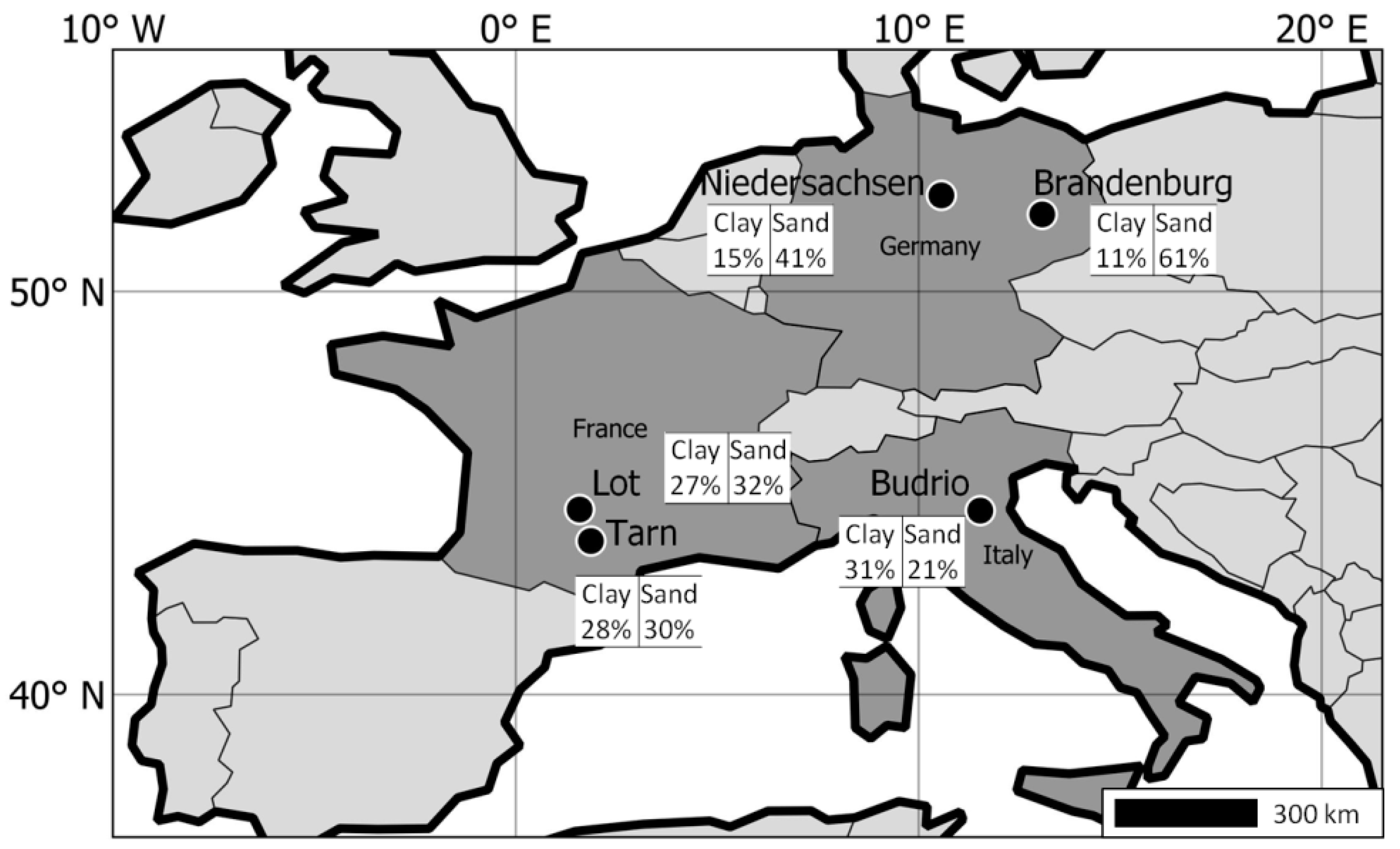
Funding

This research was funded by European Space Agency (contract 4000129870/20/I-NB, project “Irrigation+”) and Agence Nationale de la Recherche (ANR-19-CE01-0017, project “HILIAISE”).

Data Availability Statement

The irrigation dataset for Italy has been provided by CER (Canale Emiliano Romagnolo). The dataset for Germany has been provided by the Leibniz Centre for Agricultural Landscape Research (ZALF). The dataset for France has been provided separately by the Chambre d’Agriculture of the Tarn, and the Chambre d’Agriculture of the Lot under a special agreement which does not allow to distribute the data; however, we will provide all necessary connections to reach the data providers. The meteorological datasets were provided by the national rainfall network, managed by the Department of Civil and Environmental Protection (DPC) of Italy for the Italian pilot areas and by the German Weather Service (DWD) Climate Data Center (CDC).

Acknowledgments

The authors acknowledge the support from the European Space Agency (ESA) under the IRRIGATION+ project (contract n. 4000129870/20/I-NB); for further details please visit https://esairrigationplus.org/, accessed on 1 January 2022. We acknowledge the Chambre d’Agriculture of Tarn, and Lot in France for providing their dataset of irrigation. We wish to thank CER (Canale Emiliano Romagnolo) for providing the irrigation amounts over the Italian pilot site. We also thank Claas Nendel and Beate Zimmerman for providing the Germany irrigation data.

Conflicts of Interest

The authors declare no conflict of interest.

Appendix A

Appendix A.1. The Saxton Pedotransfer Equation

Saxton et al. [34] developed the following equations to estimate the Brooks–Corey parameters according to the percentage of sand (S) and clay (C):
a = e 4.396 0.0715 C 0.000488 S 2 C
b = 3.14 0.00222 C 2 0.00003484 S 2 C
Field capacity ( θ f c ) and wilting point ( θ w p ) can then be obtained at −33 Pa and 1500 Pa, respectively, with
θ f c = 15 / a 1 / b
θ w p = 0.33333 / a 1 / b

Appendix A.2. The Water Budget Used for the Detection of Irrigation

(1)
Initialization
θ fc : Field capacity
θ wp : Wilting point
T A W = θ fc     θ wp . Zr 0
T E W = θ fc   θ wp 2 . Ze
T D W = θ fc     θ wp . Zd
R E W = f i x e d   v a l u e   f o u n d   i n   F A O 56   t a b l e   19
R A W = p . T A W
D e = T E W . H i     ;   D r = T A W . H i     ; D d = T D W . H i
where TAW: Total Available Water.
TEW:
Total Evaporable Water.
TDW:
Total Deep Water.
REW:
Readily Evaporable Water.
RAW:
Readily Available Water.
De, Dr, Dd:
Depletion for upper, middle and lower bucket.
Zr0:
Initial root depth set to 10 cm.
Ze:
Evaporable depth depends of the soil. Ze is associated with the upper soil of the soil map, and can be found in FAO-56 tables.
Zd:
maximum depth as described in the soil map.
(2)
Horizontal partition according to fraction cover and fraction wet
First, the horizontal partition of the upper layer is carried on, comparing the fraction wet (fw) to the fraction cover derived from NDVI (Fcsat). The soil wetted by both irrigation and precipitation (Fewi) and the soil wetted by precipitation (Fewp) are computed as follows:
F e w i = min 1 F c s a t , f w           w i t h   1 f e w i 0.001
F e w p = 1 F c s a t f e w i               w i t h   1 f e w p 0.001
(3)
Rooting depth
Rooting depth is actualized when maximum root depth is different from minimum root depth, in fact for annual crops. Rooting Depth is derived from a linear relation to Fraction Cover which assumes that the crop will reach its full rooting at maximum fraction cover.
Z r j = F c s a t j F c s a t m a x . M a x Z r L C
where Zrj = Root Depth at day j, with Zrj > Ze+0.01.
Fcsatj = Fraction Cover of the day j.
Fcsatmax = Maximum Fraction Cover of the time series.
MaxZr(LC) = parameter for Max Root Depth of this land cover (LC).
As roots may enter different soil horizons, average wilting point and field capacity are taken from the pre-processed soil map mentioned earlier. Depletions are then actualized in the deep (Dd) and root (Dr) bucket for each day j.
D r j = [ D r j 1 + ( θ fc     θ wp ) . Zr j Zr j 1 . ( Dd TDW ) ] 0
D d j = [ D d j 1 + θ fc     θ wp . Zr j Zr j 1 . Dr TAW 0
Readily Available Water at day j (RAWj) is actualized with the equation from FAO-56, where EThb is described in part 5:
R A W j = R A W j 1 + ( T A W p + 0.04 5 E T h b j 1
(4)
Water balance, part 1
The water balance proceeds to input water from Irrigation (I) which either comes from actual or simulated irrigation and rainfall (R). The depletion of the evaporation bucket wetted with rain only (Dep), the bucket wetted with rain and irrigation (De), and the root bucket (Dr) are actualized:
Dep j = 0   Dep j 1     R   TEW
D e j = 0 D e j 1 R I f w T E W
D r j = D r j 1 R I f w             if   D r j < 0 ( D p = D r )
0<=Drj<=TAW→Dd<=TDW
(5)
Evapotranspiration
Stresses are calculated. They represent the stress after receiving water input, and after root actualization induced from the EO of the day. As remote sensing images are generally shot at mid-day, it appears to be a good compromise. Kr, the reduction coefficient for evaporation, is expressed for the fewi and fewp fractions as
K r i = T E W D e j 1 T E W R E W             for   De ( j 1 ) > = 0
K r p = T E W D e p j 1 T E W R E W             for   De p ( j 1 ) > = 0
A weighting coefficient (W) for partitioning the energy available for evaporation in the two wetted, exposed fractions of the surface layer, depending on water availability is calculated:
W = 1 / 1 + f e w p . T E W D e p f e w i . T E W D e
w i t h       0 D e T E W       ;       0 D e p T E W       ; f e w i . T E W D e p > 0.001
Evaporation coefficients are finally obtained with
K e i = Kr i . W . Kcmax Kcb > 0.05   < few i . Kcmax > k c b + 0.05 0
Ke p = Kr p . 1 W . Kcmax Kcb > 0.05   < few p . Kcmax > k c b + 0.05 0
The calculation of Ks, the reduction coefficient for basal evapotranspiration (similar to transpiration) does not change from FAO-56; it is computed with:
Ks = (TAW − (max(Dr, RAW)))/(TAW − RAW)
Evapotranspiration of the water budget is finally calculated:
ET hb = ET 0 . Ks . Kcb interp + Ke i + Ke p
where ET0 is the reference evapotranspiration computed according to the Penman–Monteith equation [20].
(6)
Water balance, part 2
We can now conclude with the calculation of the water budget.
Two coefficients (Kti, Ktp) are introduced for the purpose of separating the proportion of basal ET = Kcb.ET0 extracted as transpiration into the two fractions of the upper layer. Those coefficients vary from 0 to 1, and are calculated for 1 − Dr/TAW ≥ 0.001
K t i = 1 D e T E W 1 D r T A W . Z e Z r 0.6 1
K t p = 1 D e T E W 1 D r T A W . Z e Z r 0.6 1
Water balance is computed for the two fractions of the upper layer:
D e p j = 0 D e p j 1 + K e p . E T 0 f e w p + K t p . K c p . K s . E T 0 T E W
D e j = 0 D e j 1 + K e i + K e p . E T 0 f e w i + K t i . K c b i n t e r p . K s . E T 0 T E W
The root layer is actualized taking into account evapotranspiration:
D r i = D r i 1 + E T h b

Appendix A.3. Estimation of Surface Soil Moisture from the Buckets

According to Raes [31], 40% of the transpiration comes from the first upper quarter of soil (Zr/4). The main bucket is divided into two layers, with the upper layer having a depth equal to one-quarter of the root layer. Drtop is the depletion of water in the upper layer. TAWtop and TAWdown correspond to the total available water content in the upper and lower layers, and are computed in the same way as TAW in the FAO-56 model, but are fractioned into the upper (25%) and lower (75%) percentages. The depletion of the bottom layer Drdown is computed as the difference in depletion between the full root layer and the top root layer.
D r t o p = min   ( max   D r t o p   p r e c i p   ,   0 )   ,     T A W t o p
T A W t o p = θ f c θ w p Z r   0.25
T A W d o w n = θ f c θ w p Z r   0.75
D r t o p = min   ( max   D r t o p   p r e c i p   ,   0 )   ,     T A W t o p
T A W t o p = θ f c θ w p Z r   0.25
T A W d o w n = θ f c θ w p Z r   0.75
In a second step, Drtop is updated in accordance with known wetting events, and depletion is constrained between 0 and the maximum water content TAWtop:
D r t o p = min   ( max   D r t o p   p r e c i p   ,   0 )   ,     T A W t o p
The stress coefficient of the top layer (Kstop) was computed in the exactly the same way as Ks in the FAO-56 model, but with the water quantities of the top layer, where padjust is the average fraction of TAW that can be depleted from the root zone before water stress occurs. The transpiration of the top layer (Ttop) was then obtained with the basal crop coefficients Kcb and previously computed Kstop. In accordance with the findings of Raes [31], 40% of the transpiration is affected by the top layer. Ttop cannot be greater than the total amount of transpiration T computed with the regular FAO-56 model:
K s t o p = min ( ( T A W t o p D r t o p ) / T A W t o p 1 p a d j u s t ,   1
T t o p = m i n   ( T   ,   E T 0 K c b K s t o p 0.4 )
K s t o p = min ( ( T A W t o p D r t o p ) / T A W t o p 1 p a d j u s t ,   1
T t o p = m i n   ( T   ,   E T 0 K c b K s t o p 0.4 )
Drtop is updated by summing the evaporation (E) and the transpiration (Ttop):
D r t o p = min max   D r t o p + E + T t o p   ,   0 , T A W t o p

Appendix A.4. Estimation of Surface Soil Moisture with the Force-Restore Approach

The force-restore model receives the volumetric water content of the evaporation and root compartment, and precipitation, evaporation, and evapotranspiration daily fluxes from the FAO-56 model. The soil parameters and coefficients are computed according to [32]: θ s a t , the saturated volumetric water content (m 3 m−3), θ w p , the wilting point volumetric water content (m 3 m−3), and θ f c the field capacity volumetric water content (m 3 m−3), the slope of the retention Curve (b), and the coefficients c 2 r e f and c 1 s a t at saturation.
θ s a t = 1.08 S A N D + 494.305 10 3
θ f c = 89.0467 10 3 C L A Y 0.3496
θ w p = 35.1342 10 3 C L A Y 0.5
b = 0.137 C L A Y + 3.501
c 2 r e f = 13.815 C L A Y 0.954
c 1 s a t = 5.58 C L A Y + 84.88 10 2
The coefficients of the θ g e q equation are
a = 732.42 10 3 C L A Y 0.539
p = 0.134 C L A Y + 3.4
Then, as we are moving from a daily time step to a shorter time step, some unit conversions are needed. Fluxes of precipitation and evaporation and evapotranspiration are converted from mm.day−1 to mm.s−1. For each time step of one hour ( t s t e p = τ 24 , w i t h   τ = 86400 ) in one day, the force restore model is applied. The total soil depth (d2) is set to 0.60 m, and the evaporation depth (d1 of 0.1 m) is implicitly included in the c1sat regression equation.
First, the hourly evapotranspiration (Etr) and evaporation (Eg) are obtained from the daily values, based on the cosines of the zenith angle (coszenith). The coszenith function is the same as the one described in [20] to compute the zenithal angle for a position (lat, lon) and hour at some Julian day.
E t r = E t r d a i l y c o s z e n i t h
E g = E g d a i l y c o s z e n i t h
The variation of soil moisture is updated according to the force-restore approach from [33] derived from [19], where Pge is the hourly precipitation, which in this case supposes that the precipitation is evenly distributed over the whole day (Pg = P/24):
δ θ 2 δ t = 1 ρ d 2 P g E g E t r
θ 2 = θ 2 + t s t e p δ θ 2
x = θ 2 / θ s a t
θ e q = θ s a t x a x p 1 x 8 p
c 2 = c 2 r e f ( w 2 / ( θ s a t w 2 + 1 e 10
c 1 = c 1 s a t ( θ s a t / max θ g , θ w p b 2 + 1
δ θ g δ t = c 1 ρ P g E g c 2 τ θ g θ g e q
θ g = ( θ g + t s t e p c 1 ρ P g E g + c 2 τ θ e q ) / 1 + t s t e p c 2 τ

Appendix A.5

Table A1. The plot and seasons of the dataset.
CountryRegionPlotsCompletely Configured SeasonsBeginning YearEnding Year
GermanyBrandenburg41120162019
Niedersachsen493520182018
FranceTarn174020162019
Lot101420162019
ItalyBudrio5520162017
Total 85105

References

  1. Busschaert, L.; de Roos, S.; Thiery, W.; Raes, D.; De Lannoy, G.J.M. Net Irrigation Requirement under Different Climate Scenarios Using AquaCrop over Europe. Hydrol. Earth Syst. Sci. 2022, 26, 3731–3752. [Google Scholar] [CrossRef]
  2. Stenzel, F.; Greve, P.; Lucht, W.; Tramberend, S.; Wada, Y.; Gerten, D. Irrigation of Biomass Plantations May Globally Increase Water Stress More than Climate Change. Nat. Commun. 2021, 12, 1512. [Google Scholar] [CrossRef]
  3. Olesen, J.E.; Trnka, M.; Kersebaum, K.C.; Skjelvåg, A.O.; Seguin, B.; Peltonen-Sainio, P.; Rossi, F.; Kozyra, J.; Micale, F. Impacts and Adaptation of European Crop Production Systems to Climate Change. Eur. J. Agron. 2011, 34, 96–112. [Google Scholar] [CrossRef]
  4. Zappa, L.; Schlaffer, S.; Brocca, L.; Vreugdenhil, M.; Nendel, C.; Dorigo, W. How Accurately Can We Retrieve Irrigation Timing and Water Amounts from (Satellite) Soil Moisture? Int. J. Appl. Earth Obs. Geoinf. 2022, 113, 102979. [Google Scholar] [CrossRef]
  5. Massari, C.; Modanesi, S.; Dari, J.; Gruber, A.; De Lannoy, G.J.M.; Girotto, M.; Quintana-Seguí, P.; Le Page, M.; Jarlan, L.; Zribi, M.; et al. A Review of Irrigation Information Retrievals from Space and Their Utility for Users. Remote Sens. 2021, 13, 4112. [Google Scholar] [CrossRef]
  6. Jalilvand, E.; Tajrishy, M.; Ghazi Zadeh Hashemi, S.A.; Brocca, L. Quantification of Irrigation Water Using Remote Sensing of Soil Moisture in a Semi-Arid Region. Remote Sens. Environ. 2019, 231, 111226. [Google Scholar] [CrossRef]
  7. Brocca, L.; Tarpanelli, A.; Filippucci, P.; Dorigo, W.; Zaussinger, F.; Gruber, A.; Fernández-Prieto, D. How Much Water Is Used for Irrigation? A New Approach Exploiting Coarse Resolution Satellite Soil Moisture Products. Int. J. Appl. Earth Obs. Geoinf. 2018, 73, 752–766. [Google Scholar] [CrossRef]
  8. Ulaby, F.T.; Moore, R.K.; Fung, A.K. Microwave Remote Sensing: Active and Passive. Volume III: From Theory to Applications; Haralick, R.M., Simonett, D.S., Eds.; Artech Hou.: Dedham, MA, USA, 1986. [Google Scholar]
  9. Kalma, J.D.; McVicar, T.R.; McCabe, M.F. Estimating Land Surface Evaporation: A Review of Methods Using Remotely Sensed Surface Temperature Data. Surv. Geophys. 2008, 29, 421–469. [Google Scholar] [CrossRef]
  10. Olivera-Guerra, L.; Merlin, O.; Er-Raki, S. Irrigation Retrieval from Landsat Optical/Thermal Data Integrated into a Crop Water Balance Model: A Case Study over Winter Wheat Fields in a Semi-Arid Region. Remote Sens. Environ. 2020, 239, 111627. [Google Scholar] [CrossRef] [Green Version]
  11. Bazzi, H.; Baghdadi, N.; Fayad, I.; Zribi, M.; Belhouchette, H.; Demarez, V. Near Real-Time Irrigation Detection at Plot Scale Using Sentinel-1 Data. Remote Sens. 2020, 12, 1456. [Google Scholar] [CrossRef]
  12. Bazzi, H.; Baghdadi, N.; Najem, S.; Jaafar, H.; Le Page, M.; Zribi, M.; Faraslis, I.; Spiliotopoulos, M. Detecting Irrigation Events over Semi-Arid and Temperate Climatic Areas Using Sentinel-1 Data: Case of Several Summer Crops. Agronomy 2022, 12, 2725. [Google Scholar] [CrossRef]
  13. Le Page, M.; Jarlan, L.; El Hajj, M.M.; Zribi, M.; Baghdadi, N.; Boone, A. Potential for the Detection of Irrigation Events on Maize Plots Using Sentinel-1 Soil Moisture Products. Remote Sens. 2020, 12, 1621. [Google Scholar] [CrossRef]
  14. El Hajj, M.; Baghdadi, N.; Zribi, M.; Bazzi, H. Synergic Use of Sentinel-1 and Sentinel-2 Images for Operational Soil Moisture Mapping at High Spatial Resolution over Agricultural Areas. Remote Sens. 2017, 9, 1292. [Google Scholar] [CrossRef] [Green Version]
  15. Ouaadi, N.; Jarlan, L.; Khabba, S.; Ezzahar, J.; Le Page, M.; Merlin, O. Irrigation Amounts and Timing Retrieval through Data Assimilation of Surface Soil Moisture into the FAO-56 Approach in the South Mediterranean Region. Remote Sens. 2021, 13, 2667. [Google Scholar] [CrossRef]
  16. Ouaadi, N.; Jarlan, L.; Ezzahar, J.; Zribi, M.; Khabba, S.; Bouras, E.; Bousbih, S.; Frison, P. Monitoring of Wheat Crops Using the Backscattering Coe Ffi Cient and the Interferometric Coherence Derived from Sentinel-1 in Semi-Arid Areas. Remote Sens. Environ. 2020, 251, 112050. [Google Scholar] [CrossRef]
  17. Brombacher, J.; Silva, I.R.d.O.; Degen, J.; Pelgrum, H. A Novel Evapotranspiration Based Irrigation Quantification Method Using the Hydrological Similar Pixels Algorithm. Agric. Water Manag. 2022, 267, 107602. [Google Scholar] [CrossRef]
  18. Allen, R.; Pereira, L.; Smith, M.; Raes, D.; Wright, J. FAO-56 Dual Crop Coefficient Method for Estimating Evaporation from Soil and Application Extensions. J. Irrig. Drain. Eng. 2005, 131, 2–13. [Google Scholar] [CrossRef] [Green Version]
  19. Deardorff, J.W. Efficient Prediction of Ground Surface Temperature and Moisture, with Inclusion of a Layer of Vegetation. J. Geophys. Res. 1978, 83, 1889–1903. [Google Scholar] [CrossRef] [Green Version]
  20. Allen, R.G.; Pereira, L.; Raes, D.; Smith, M. FAO Irrigation and Drainage N°56: Guidelines for Computing Crop Water Requirements; FAO: Rome, Italy, 1998; Volume 300, ISBN 92-5-104219-5. [Google Scholar]
  21. Le Page, M.; Toumi, J.; Khabba, S.; Hagolle, O.; Tavernier, A.; Kharrou, M.; Er-Raki, S.; Huc, M.; Kasbani, M.; Moutamanni, A.; et al. A Life-Size and Near Real-Time Test of Irrigation Scheduling with a Sentinel-2 Like Time Series (SPOT4-Take5) in Morocco. Remote Sens. 2014, 6, 11182–11203. [Google Scholar] [CrossRef] [Green Version]
  22. Hengl, T.; Mendes de Jesus, J.; Heuvelink, G.B.M.; Ruiperez Gonzalez, M.; Kilibarda, M.; Blagotić, A.; Shangguan, W.; Wright, M.N.; Geng, X.; Bauer-Marschallinger, B.; et al. SoilGrids250m: Global Gridded Soil Information Based on Machine Learning. PLoS ONE 2017, 12, e0169748. [Google Scholar] [CrossRef] [Green Version]
  23. Zappa, L.; Schlaffer, S.; Bauer-Marschallinger, B.; Nendel, C.; Zimmerman, B.; Dorigo, W. Detection and Quantification of Irrigation Water Amounts at 500 m Using Sentinel-1 Surface Soil Moisture. Remote Sens. 2021, 13, 1727. [Google Scholar] [CrossRef]
  24. Muñoz-Sabater, J.; Dutra, E.; Agustí-Panareda, A.; Albergel, C.; Arduini, G.; Balsamo, G.; Boussetta, S.; Choulga, M.; Harrigan, S.; Hersbach, H.; et al. ERA5-Land: A State-of-the-Art Global Reanalysis Dataset for Land Applications. Earth Syst. Sci. Data 2021, 13, 4349–4383. [Google Scholar] [CrossRef]
  25. Main-Knorn, M.; Pflug, B.; Louis, J.; Debaecker, V.; Müller-Wilm, U.; Gascon, F. Sen2Cor for Sentinel-2. In Image and Signal Processing for Remote Sensing XXIII; Bruzzone, L., Bovolo, F., Benediktsson, J.A., Eds.; SPIE: Warsaw, Poland, 2017; p. 3. [Google Scholar]
  26. Doxani, G.; Vermote, E.; Roger, J.-C.; Gascon, F.; Adriaensen, S.; Frantz, D.; Hagolle, O.; Hollstein, A.; Kirches, G.; Li, F.; et al. Atmospheric Correction Inter-Comparison Exercise. Remote Sens. 2018, 10, 352. [Google Scholar] [CrossRef] [Green Version]
  27. Skakun, S.; Wevers, J.; Brockmann, C.; Doxani, G.; Aleksandrov, M.; Batič, M.; Frantz, D.; Gascon, F.; Gómez-Chova, L.; Hagolle, O.; et al. Cloud Mask Intercomparison EXercise (CMIX): An Evaluation of Cloud Masking Algorithms for Landsat 8 and Sentinel-2. Remote Sens. Environ. 2022, 274, 112990. [Google Scholar] [CrossRef]
  28. Savitzky, A.; Golay, M.J.E. Smoothing and Differentiation of Data by Simplified Least Squares Procedures. Anal. Chem. 1964, 36, 1627–1639. [Google Scholar] [CrossRef]
  29. Attema, E.P.W.; Ulaby, F.T. Vegetation Modeled as a Water Cloud. Radio Sci. 1978, 13, 357–364. [Google Scholar] [CrossRef]
  30. Simonneaux, V.; Le Page, M.; Helson, D.; Thomas, S. Estimation Spatialisée de l’évapotranspiration Des Cultures Irriguées Par Télédétection: Application à La Gestion de l’irrigation Dans La Plaine Du Haouz. Secheresse 2009, 20, 123–130. [Google Scholar] [CrossRef] [Green Version]
  31. Raes, D. BUDGET, a Soil Water and Salt Balance Model: Reference Manual. K.U.Leuven, Department Land Management: Leuven, Belgium. Available online: https://iupware.be/wp-content/uploads/2016/03/budget_manual.pdf. (accessed on 1 January 2019).
  32. Noilhan, J.; Mahfouf, J.F. The ISBA Land Surface Parameterization Scheme. Glob. Planet. Chang. 1996, 13, 145–159. [Google Scholar] [CrossRef]
  33. Noilhan, J.; Planton, S. A Simple Parameterization of Land Surface Processes for Meteorological Models. Mon. Weather Rev. 1989, 117, 536–549. [Google Scholar] [CrossRef]
  34. Saxton, K.E.; Rawls, W.J.; Romberger, J.S.; Papendick, R.I. Estimating Generalized Soil-Water Characteristics from Texture. Soil Sci. Soc. Am. J. 1986, 50, 1031–1036. [Google Scholar] [CrossRef]
  35. Paolini, G.; Escorihuela, M.J.; Merlin, O.; Sans, M.P.; Bellvert, J. Classification of Different Irrigation Systems At Field Scale Using Time-Series of Remote Sensing Data. IEEE J. Sel. Top. Appl. Earth Obs. Remote Sens. 2022, 15, 10055–10072. [Google Scholar] [CrossRef]
  36. Portmann, F.T.; Siebert, S.; Döll, P. MIRCA2000—Global Monthly Irrigated and Rainfed Crop Areas around the Year 2000: A New High—Resolution Data Set for Agricultural and Hydrological Modeling. Glob. Biogeochem. Cycles 2010, 24, 1–24. [Google Scholar] [CrossRef]
  37. Gao, B.C. NDWI—A Normalized Difference Water Index for Remote Sensing of Vegetation Liquid Water from Space. Remote Sens. Environ. 1996, 58, 257–266. [Google Scholar] [CrossRef]
Figure 1. Regions location and average soil texture from the dataset’s fields.
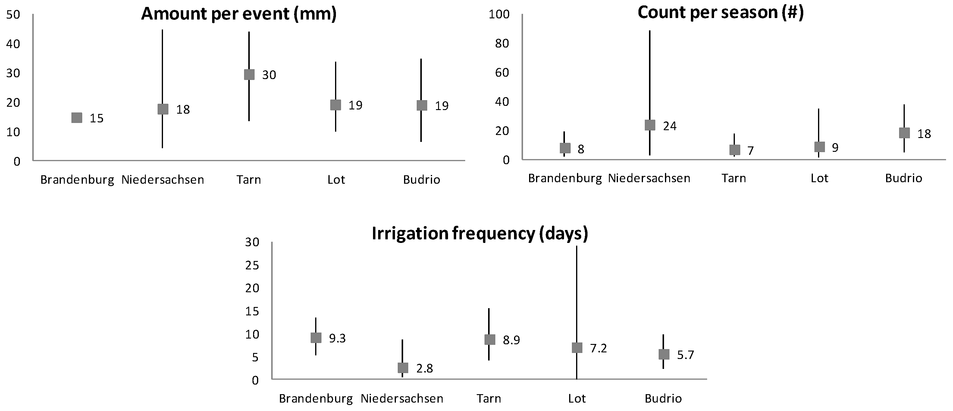
Remotesensing 15 01449 g001
Figure 2. Statistics of irrigation events. The bars show the minimum and maximum. The square and number show the average value.
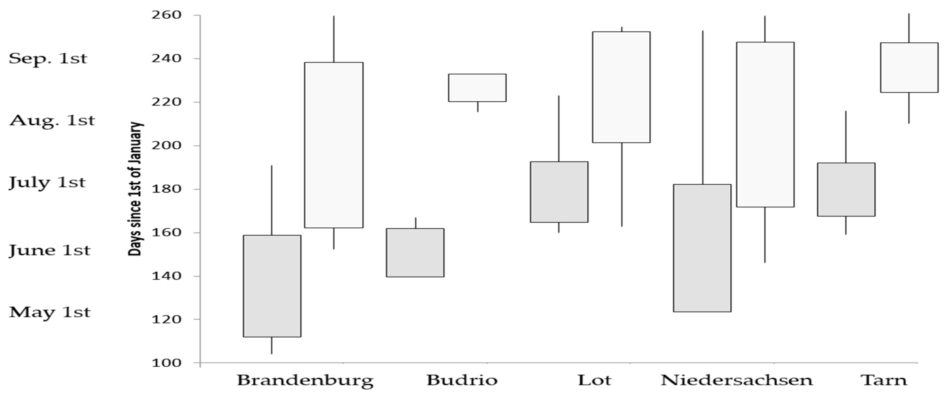
Remotesensing 15 01449 g002
Figure 3. Start (gray color) and end (white color) of irrigation season per region. The box shows the mean date plus or minus one standard deviation. The line indicates the extremes, i.e., the minimum and maximum date of beginning and end of the irrigation season.
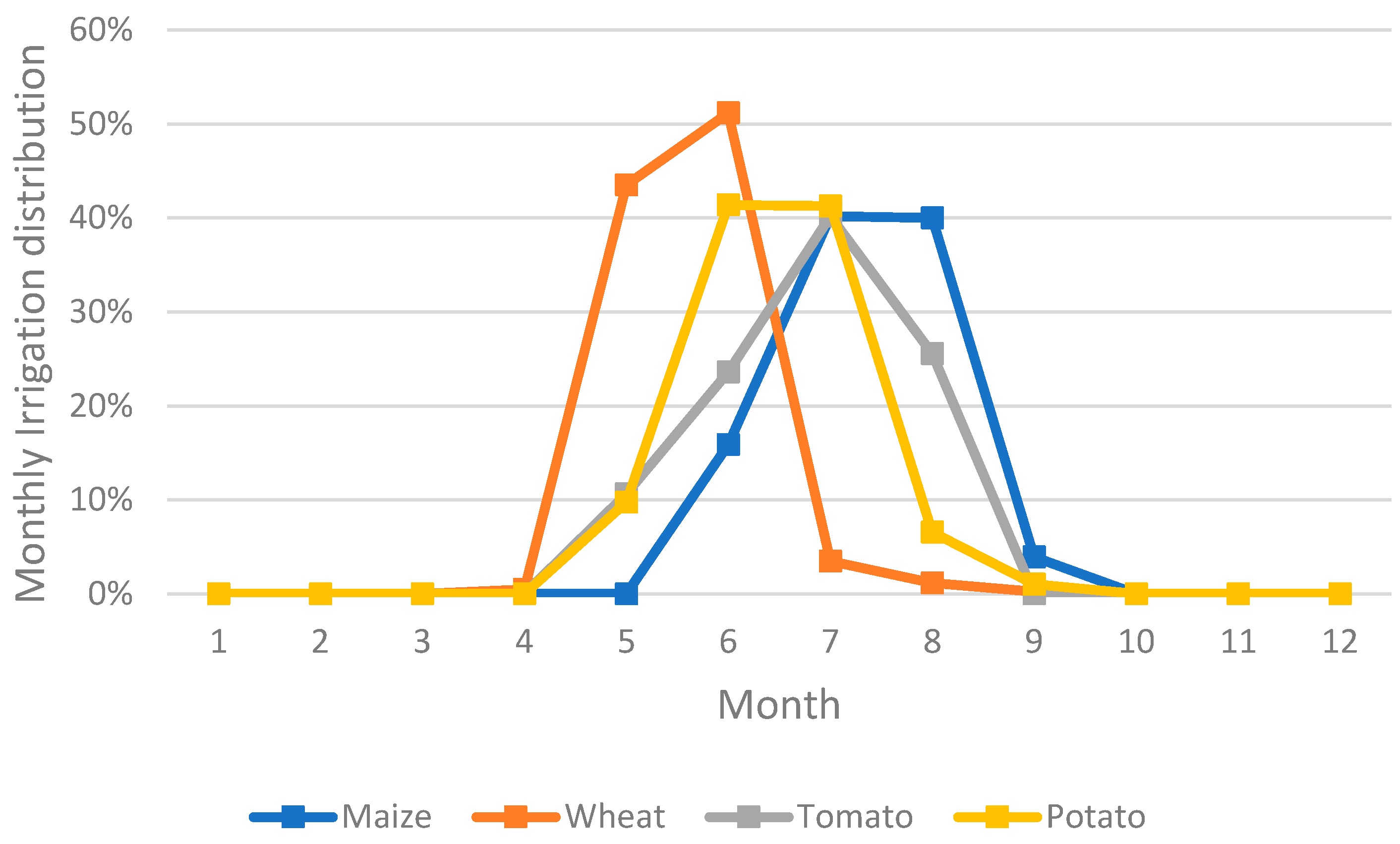
Remotesensing 15 01449 g003
Figure 4. Irrigation distribution of the four main crops of the dataset.
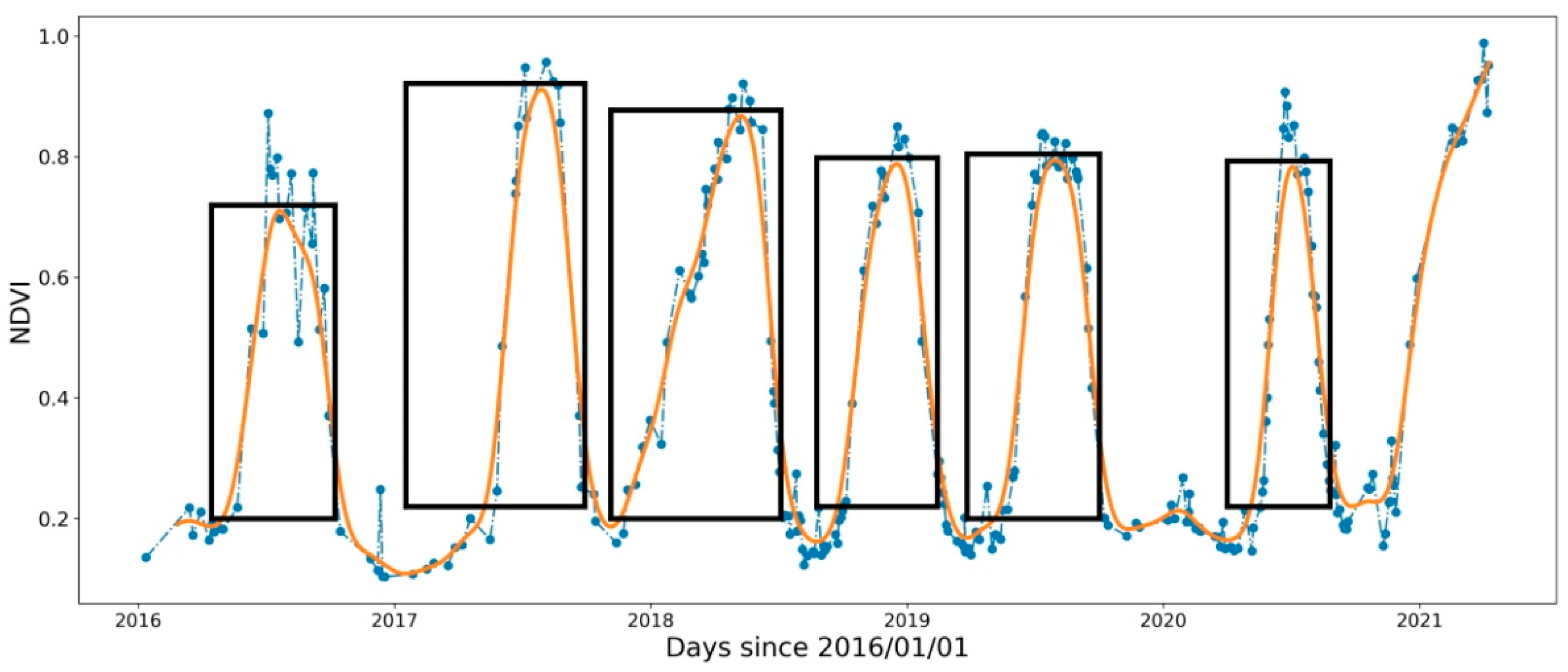
Remotesensing 15 01449 g004
Figure 5. Example of identification of the start and end of the crop season from Sentinel-2 NDVI time series. The dashed blue line is the original Sentinel-2 time series of NDVI. The orange line is the filtered NDVI. The black boxes are the estimated crop seasons.
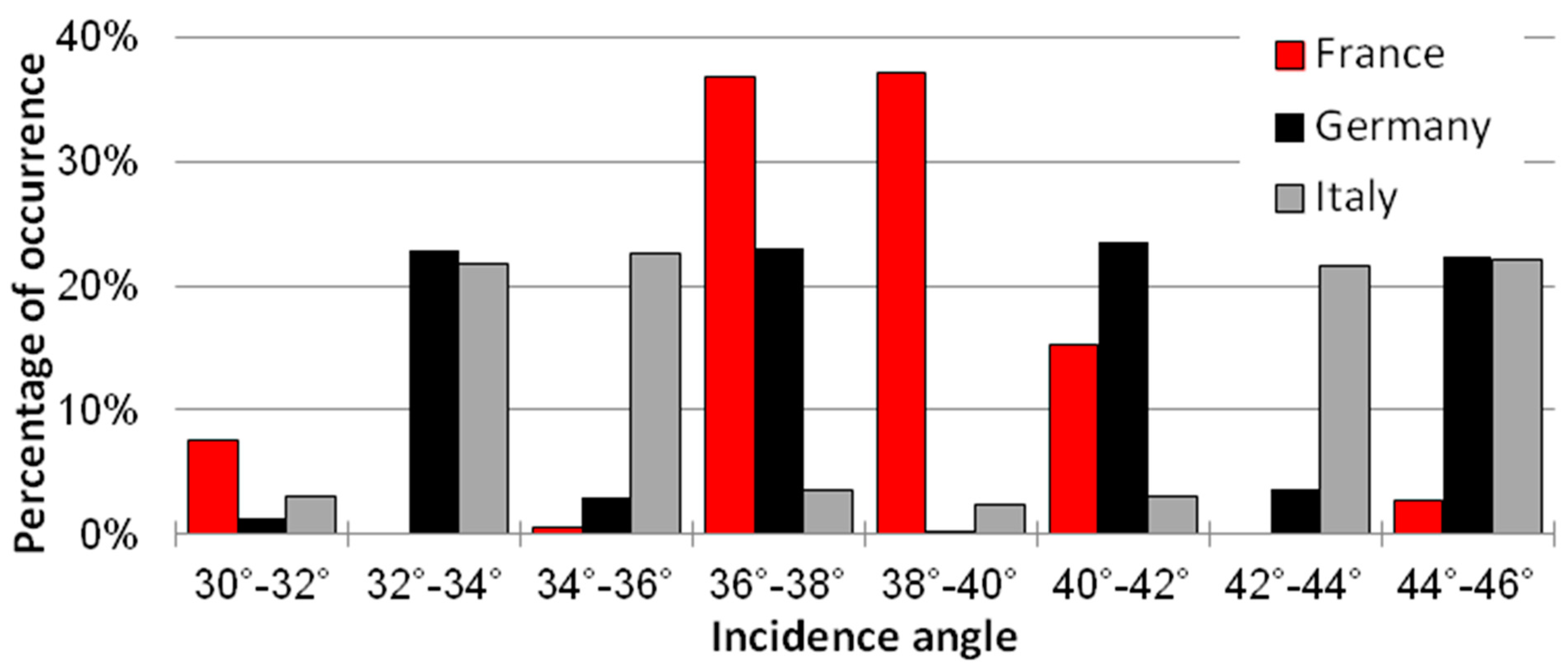
Remotesensing 15 01449 g005
Figure 6. Incidence angle Sentinel-1 A and B acquisitions per country studied.
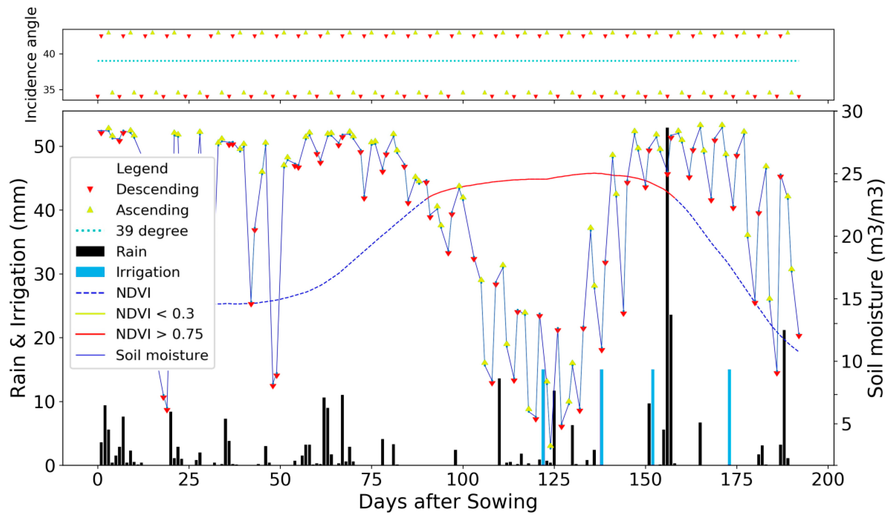
Remotesensing 15 01449 g006
Figure 7. Lower panel: An example of the time series used for the timing of irrigation. The main graph shows the rainfall and irrigation events as black and blue bars, respectively. The NDVI is drawn with a dark-blue dashed line when lower than 0.75 and red dashes when higher than 0.75. The S2SM product is drawn with yellow arrows (ascending orbit) and red arrows (descending orbit); Upper panel: the incidence angle of acquisition is shown.
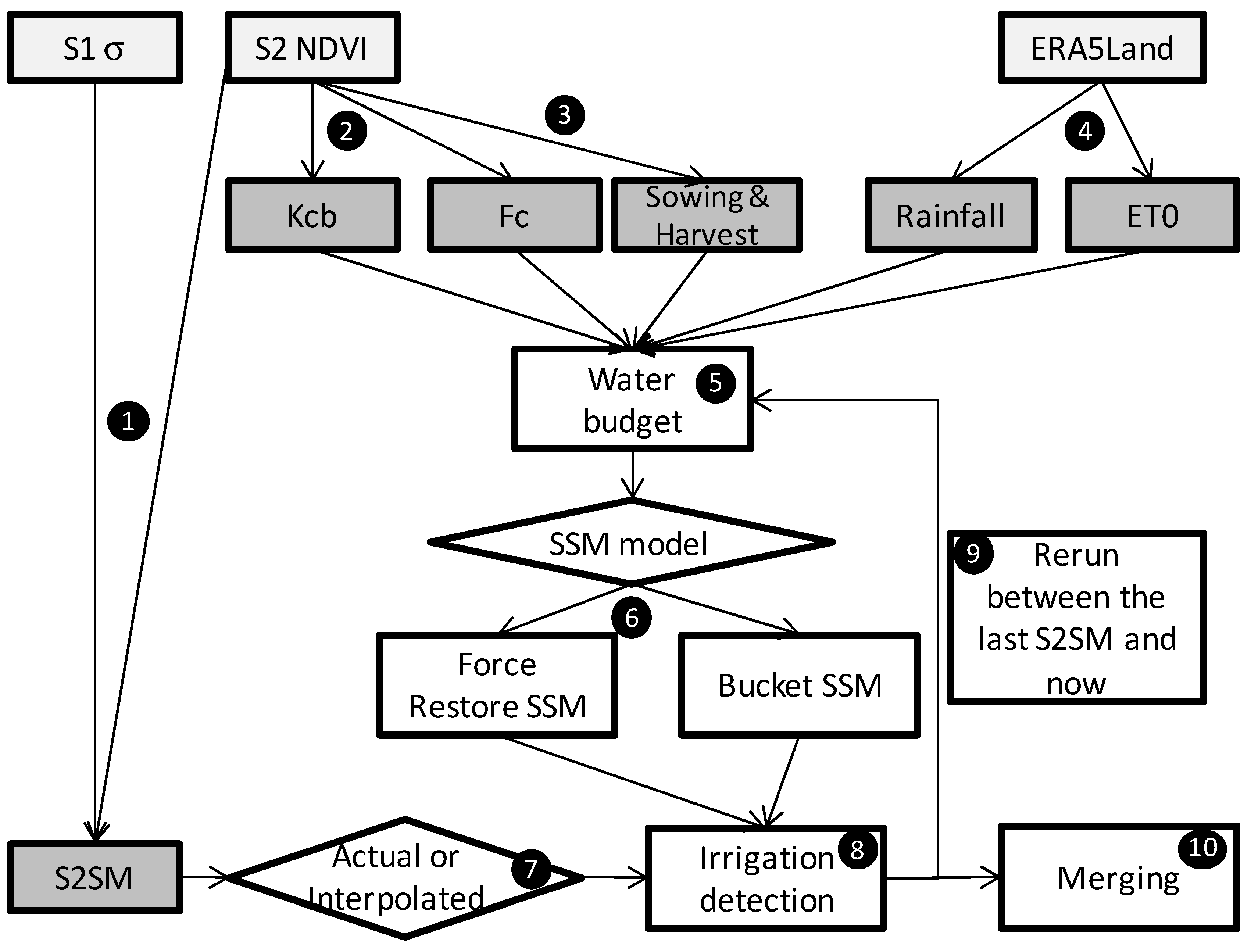
Remotesensing 15 01449 g007
Figure 8. The workflow of this article is based on three datasets (in light gray boxes). The steps 1 to 4 allow to obtain intermediate variables, with, on one side, the Surface Soil Moisture product obtained from satellite observations (S2SM), and, on the other side, the variables that will allow the computing of a water budget for the estimation of the surface soil moisture (basal crop coefficient (Kcb), Fraction cover (Fc), sowing and harvest date, precipitation and reference evapotranspiration (ET0)). Steps 5 to 9 are the irrigation detection steps. The two diamonds (6 and 7) indicate sub-methods for dealing with soil moisture observation and soil moisture estimation, respectively. The final step (10) consists of merging results.
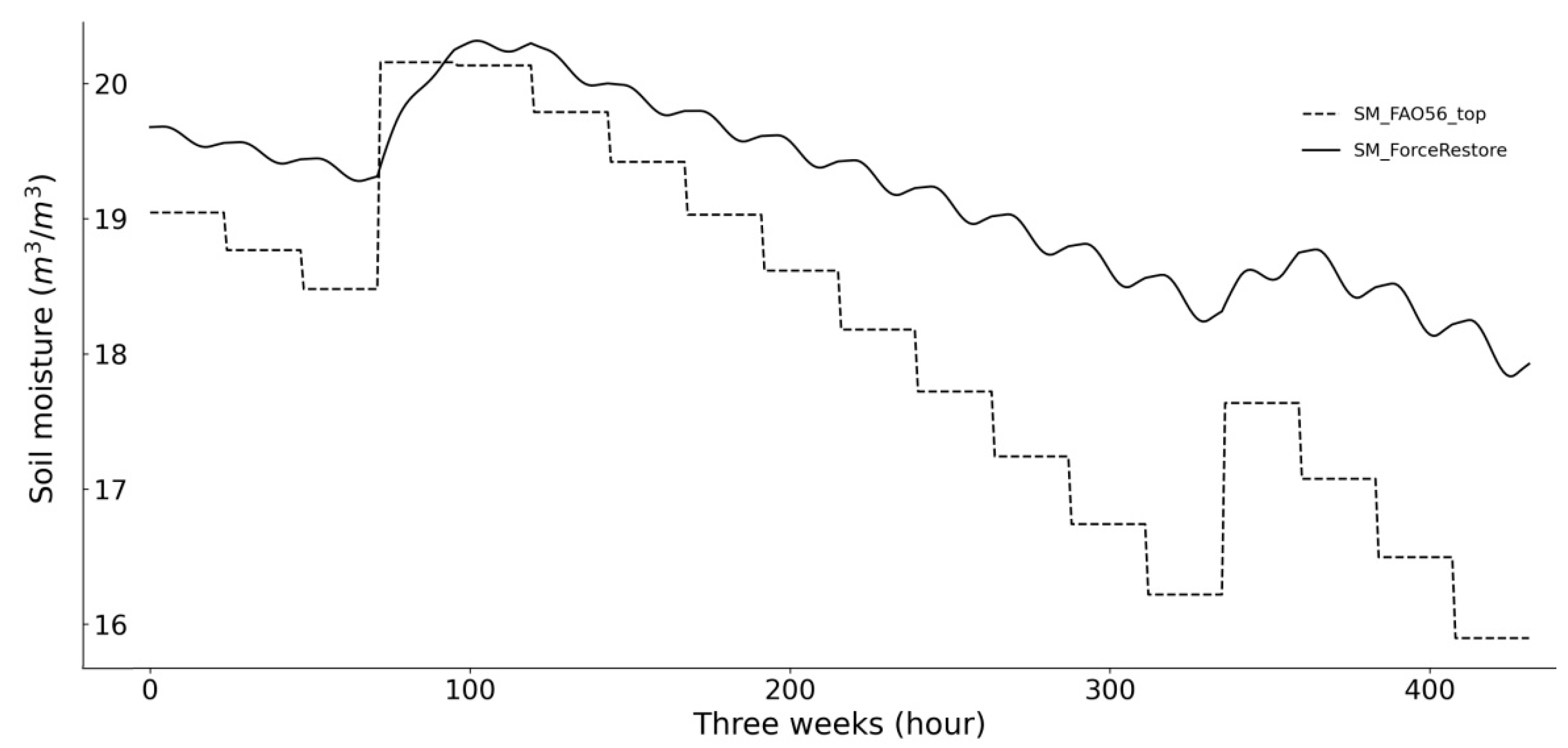
Remotesensing 15 01449 g008
Figure 9. Example of SSM dynamic simulated by the modified FAO-56 (dashed line) and the force-restore model (dash and point line) after a wetting event.
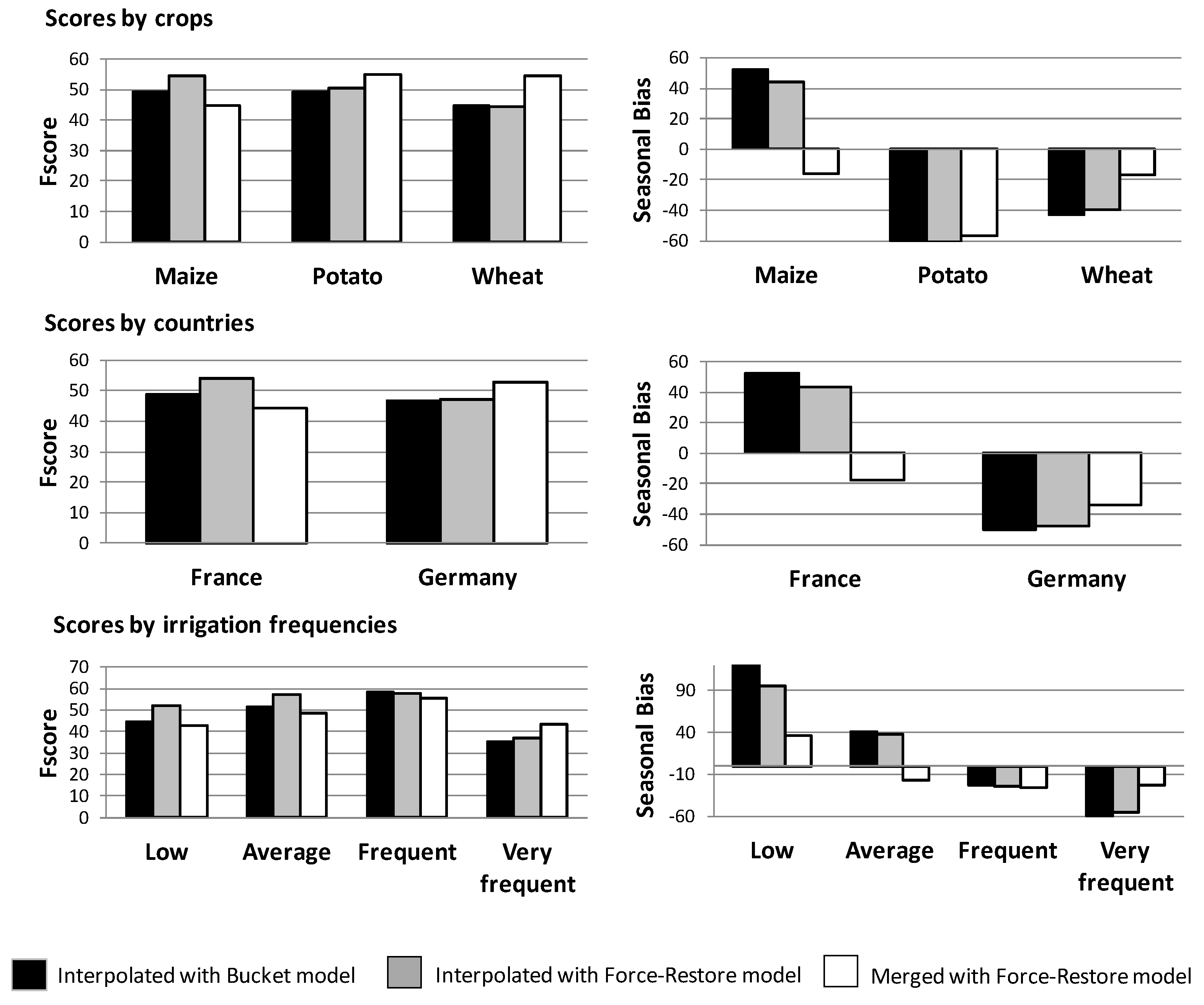
Remotesensing 15 01449 g009
Figure 10. Comparison of the interpolated method with all data and the original SSM model, the interpolated method with all data and the force-restore model, and the merged runs with the force restore. On the left side, the histograms show the F-scores. On the right side, the histograms show the seasonal biases. From top to bottom, the results are shown for crops, countries, and irrigation frequencies.
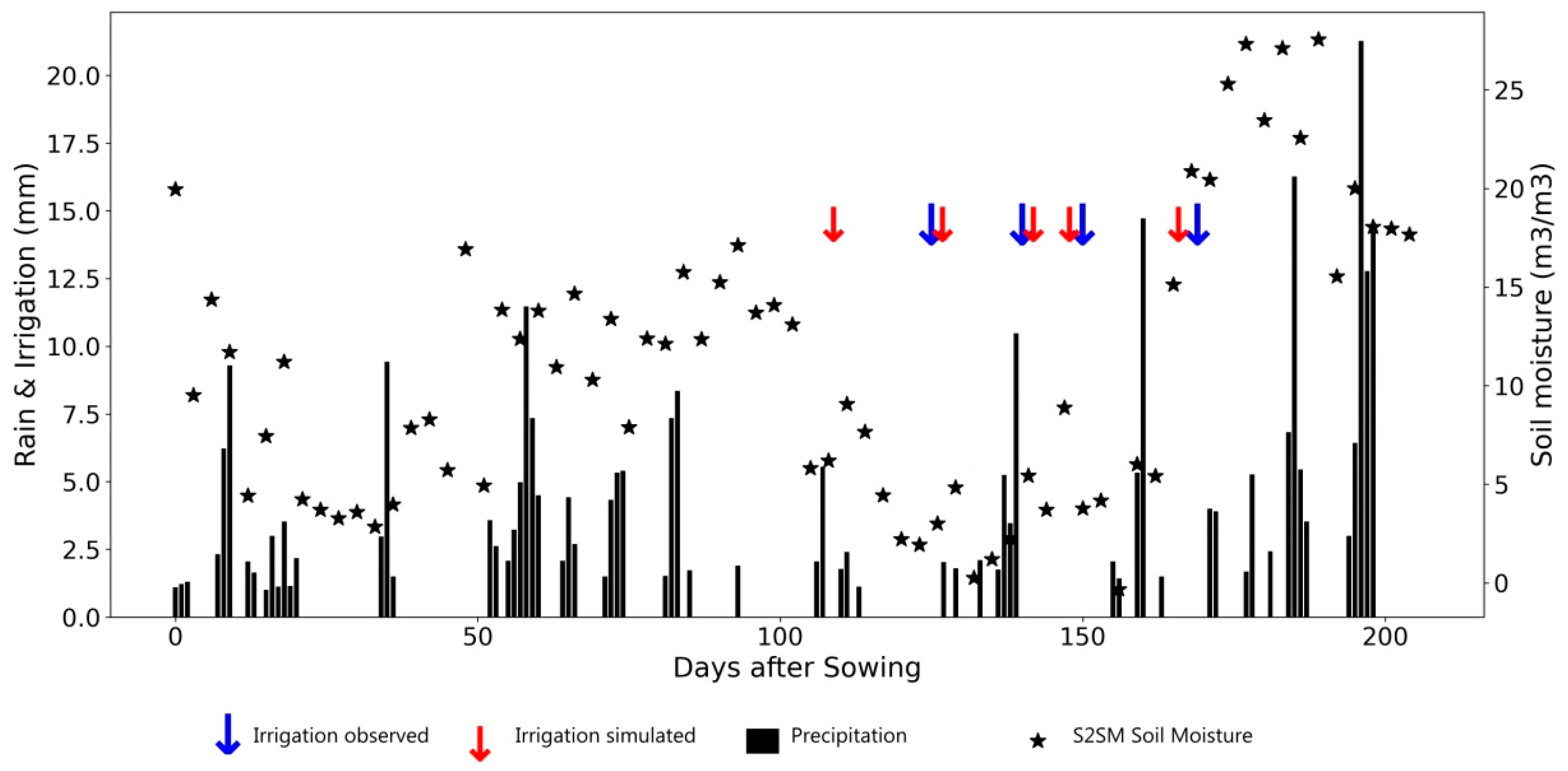
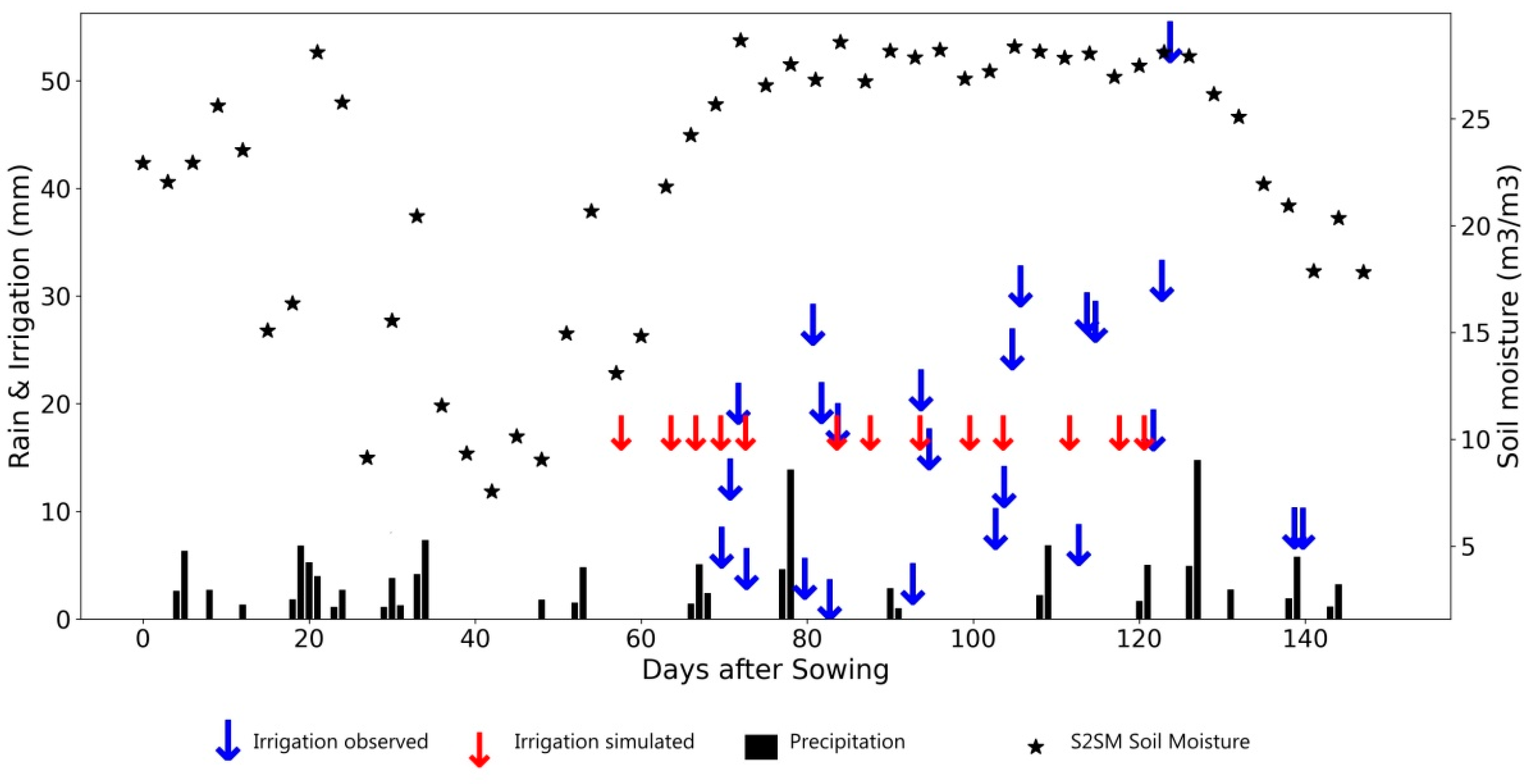
Remotesensing 15 01449 g010
Figure 11. Example of detection events of low frequency and average amounts of irrigation on winter rye in Brandenburg in 2017. Irrigation observations are indicated by blue arrows (Irri_obs); irrigation simulations are indicated by red arrows (Irri_simu). Actual rainfall events are shown with black bars. The interpolated S2SM product (selected every three days) is shown by stars. Vegetation (Kcb) is shown with blue dashed lines and the model predictions of soil moisture are also shown (SM_FAO, and SM_top).
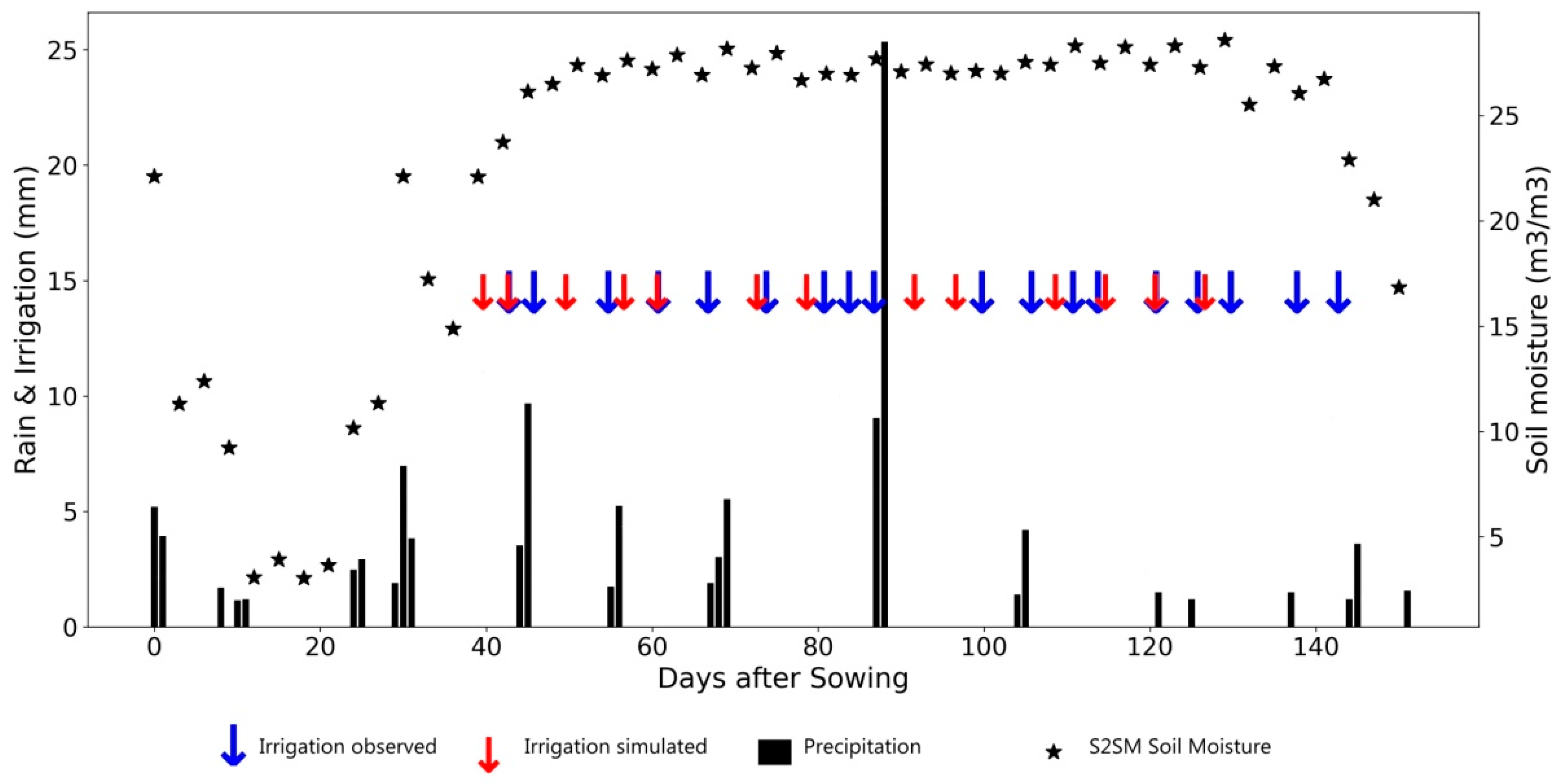
Remotesensing 15 01449 g011
Figure 12. Same as Figure 12 for a potato field in Brandenburg in 2018 (high irrigation frequency and average irrigation amounts).
Remotesensing 15 01449 g012
Figure 13. Same as Figure 12 for a potato field in Niedersachsen in 2018 (high irrigation frequency and low amounts of irrigation).
Remotesensing 15 01449 g013
Table 1. The number of seasons per crop and region in the dataset.
GermanyFranceItaly
Crop Brand.Nied.LotTarnBudrioTotal
VegetablesSoybean 11 1116
Asparragus 1 1
Tomato 33
Pea1 1
CerealsTriticale 4 470
Winter Rye3 3
Winter wheat49 13
Maize2 29233
Maize (seed) 7 7
Summer barley 10 10
FodderMaize (forrage) 7 713
Rapeseed13 4
Grass2 2
TubersPotato212 1424
Sugar beet 10 10
OthersTobacco 8 810
Walnut 2 2
Table 2. Scores (F-score, bias) of the bucket approach according to different configurations (orbit, incidence angle, crop, country, irrigation frequency), and the level of NDVI (all data, small NDVI values, high NDVI values).
FscoreBias
ConfigurationAll NDVILarge NDVISmall NDVIAll NDVILarge NDVISmall NDVI
OrbitASC (6PM)322824−221−68−69
DES (6AM)353028−167−64−62
Incidence angle37-41352926−131−59−55
Other342927−228−69−69
CropMaize403430−42−41−7
Potato322527−402−82−79
Wheat312724−225−70−68
CountryFrance403332−41−41−8
Germany322824−277−74−73
Irrigation FrequencyLow4442344−1258
Average443927−49−41−21
Frequent383032−177−68−61
Very Frequent242121−435−83−80
Table 3. Scores (F-score, bias) of the merging of irrigations runs according to 3 merging windows (one day, two days, three days) and according to crops, country, and irrigation frequency.
MergingFscoreBias
Configuration1 Day2 Days3 Days1 Day2 Days3 Days
CropMaize454545−16−19−22
Potato555345−57−60−68
Wheat514742−16−27−40
CountryFrance444545−18−20−22
Germany534944−34−42−53
Irrigation FrequencyLow434444363025
Average494949−17−20−24
Frequent565349−24−32−41
Very Frequent434033−53−58−67
Table 4. Scores (F-score, bias) of the force-restore model according to irrigation frequency and NDVI.
Force-Restore Model Fscore Bias
ConfigurationAll NDVILarge NDVISmall NDVIAll NDVILarge NDVISmall NDVI
Irrigation FrequencyLow5051292917118
Average504829−11−187
Frequent413436−119−58−48
Very Frequent262224−337−80−74
Table 5. Comparison of scores between the initial bucket soil water budget and the force-restore—FR—approach (score FR minus score Bucket), according to different configurations (Crop, Country, Irrigation frequency, Acquisition, Angle).
CropprecisionrecallF-score CountryprecisionrecallF-score
Maize−2.913.36.6 France−3.113.26.3
Potato−2.62.12.6 Germany−7.13.32.4
Wheat−9.43.32.0
AcquisitionprecisionrecallF-score
Irrigation frequencyprecisionrecallF-score ASC−3.57.35.0
DES−7.45.72.7
Low−1.915.36.1
Average−2.311.25.8 AngleprecisionrecallF-score
Frequent−8.04.63.1 37–41−3.010.36.0
Very−7.42.92.3 Other−7.83.82.0
Table 6. Scores (F-score, bias) of the interpolated approach according to different configurations orbit, incidence angle, crop, country, irrigation frequency), and the level of NDVI (all data, small NDVI values, high NDVI values).
Fscore Bias
ConfigurationAll NDVILarge NDVISmall NDVIAll NDVILarge NDVISmall NDVI
CropMaize494235452872
Potato494348−60−70−51
Wheat454036−43−43−40
CountryFrance484133392857
Germany474240−50−54−45
Irrigation FrequencyLow45473110274168
Average524435352451
Frequent584844−24−25−21
Very Frequent342833−61−70−53
Disclaimer/Publisher’s Note: The statements, opinions and data contained in all publications are solely those of the individual author(s) and contributor(s) and not of MDPI and/or the editor(s). MDPI and/or the editor(s) disclaim responsibility for any injury to people or property resulting from any ideas, methods, instructions or products referred to in the content.

