
The Role of Aerosol Concentration on Precipitation in a Winter Extreme Mixed-Phase System: The Case of Storm Filomena

 , , , and
Abstract
:1. Introduction
2. Methodology
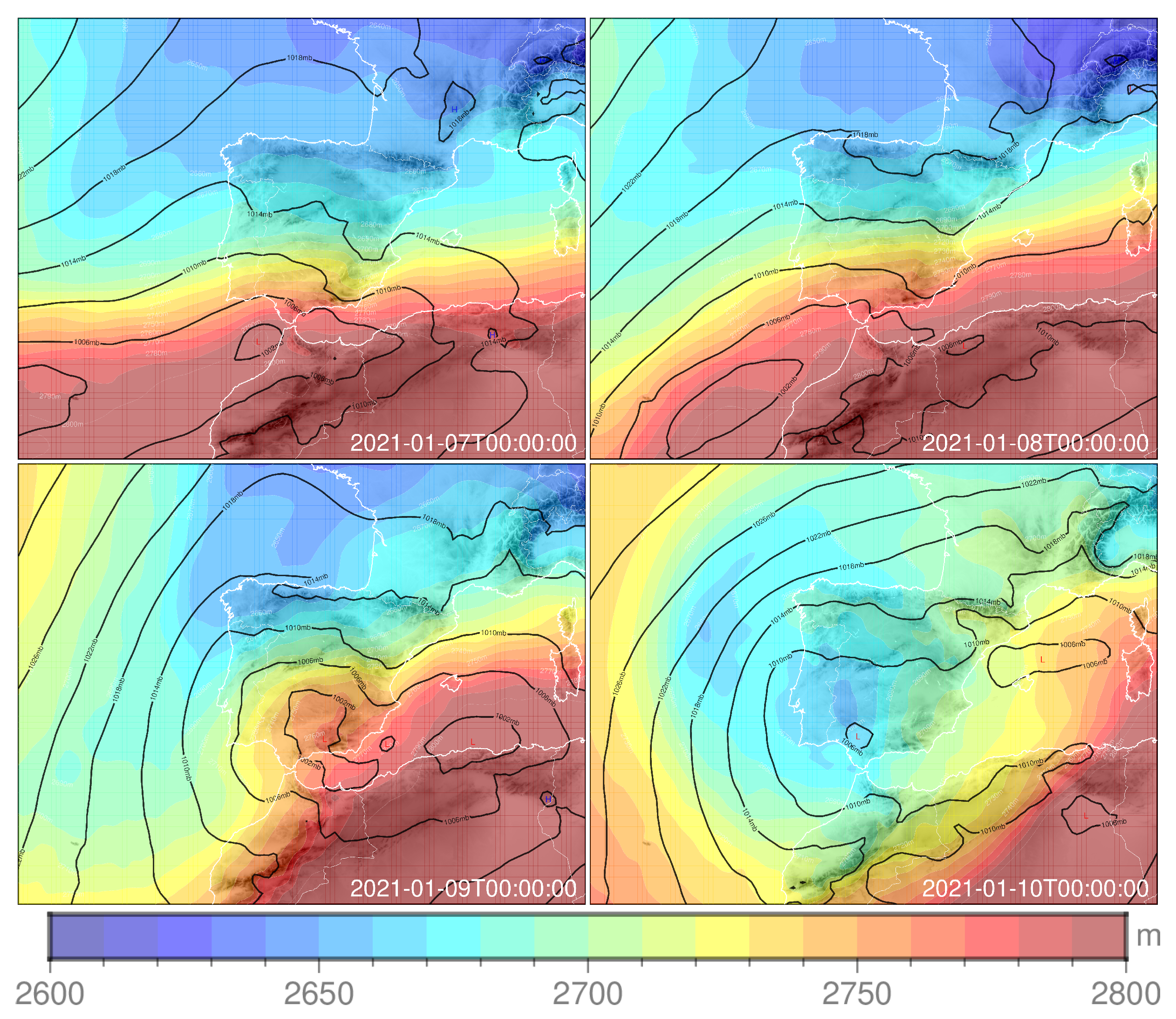
2.1. Storm Filomena
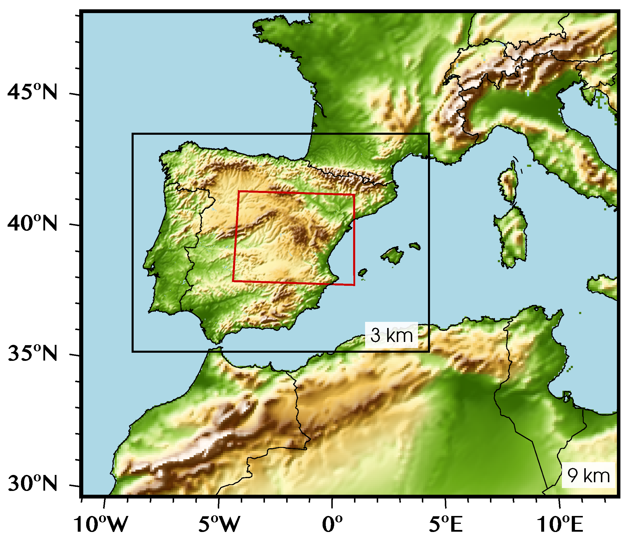
2.2. Model Configuration
2.3. Microphysics Setup
3. Results
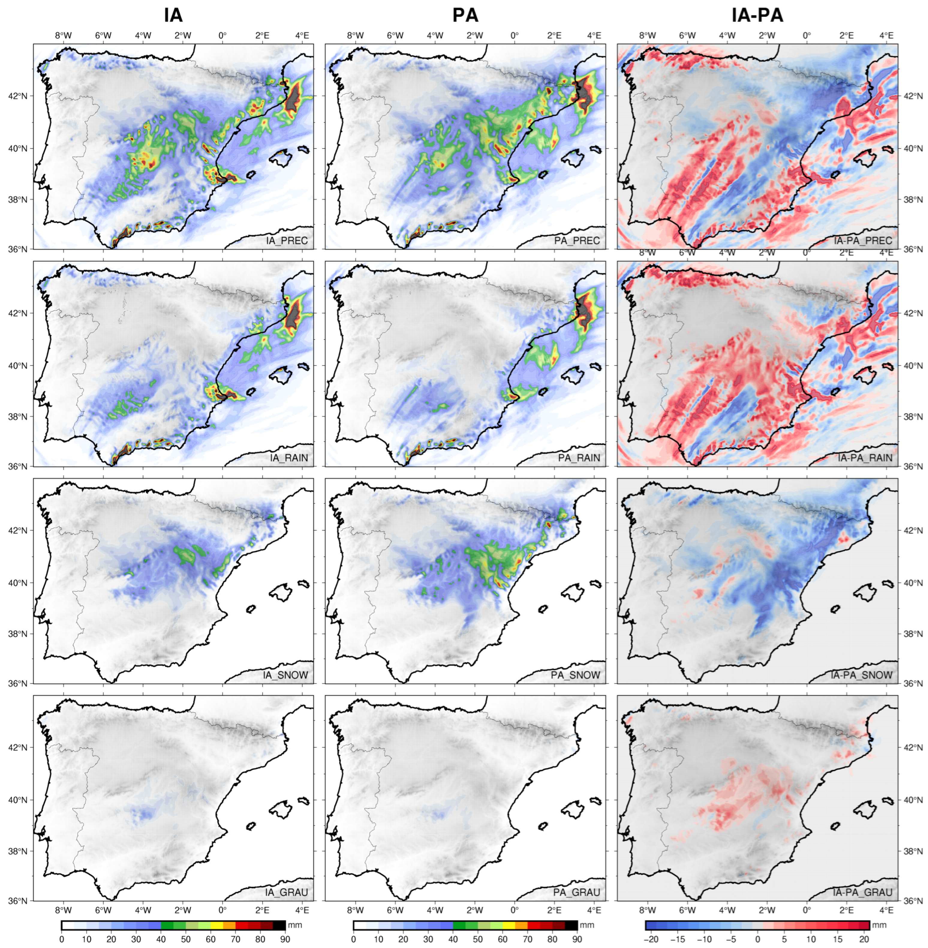
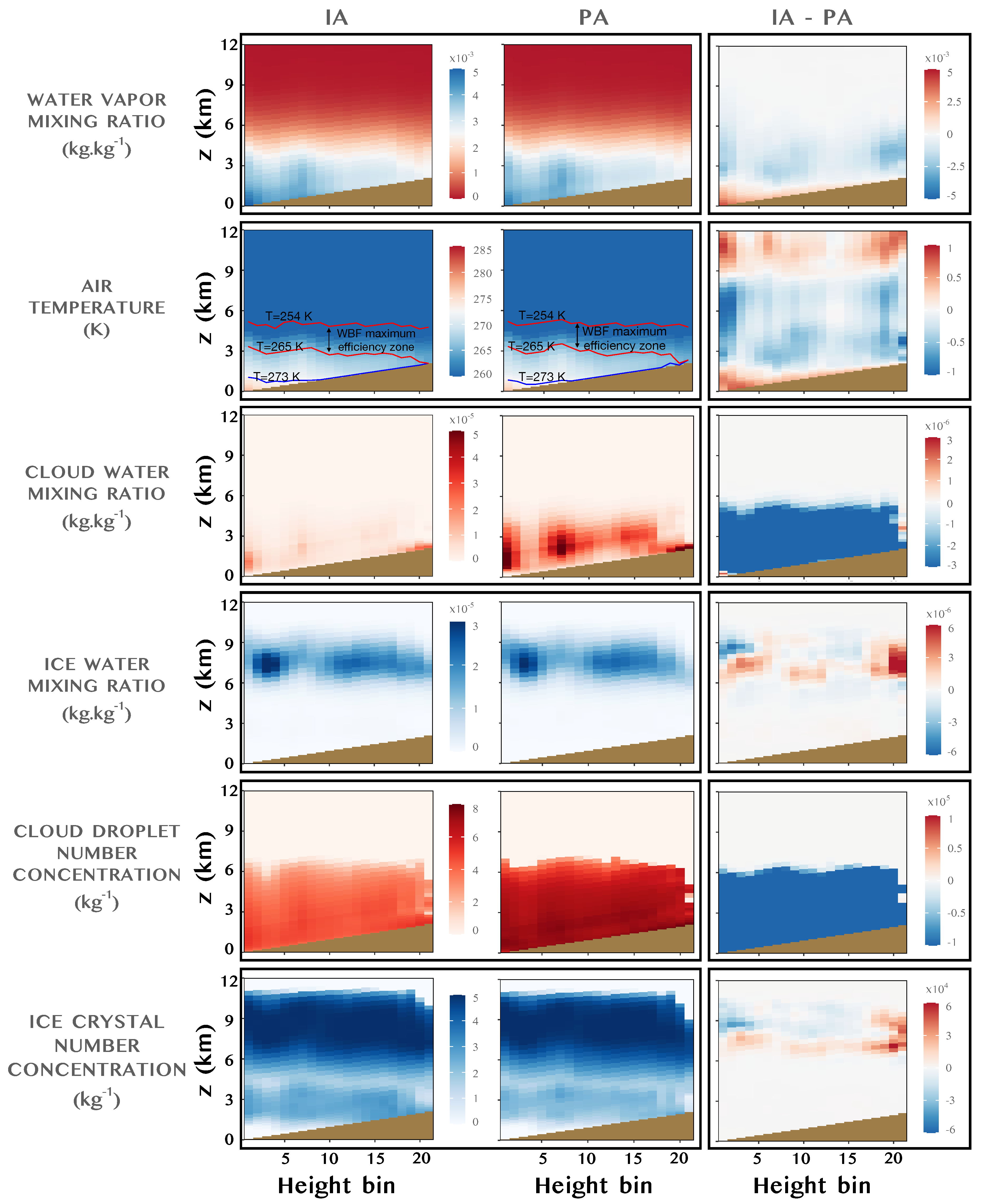
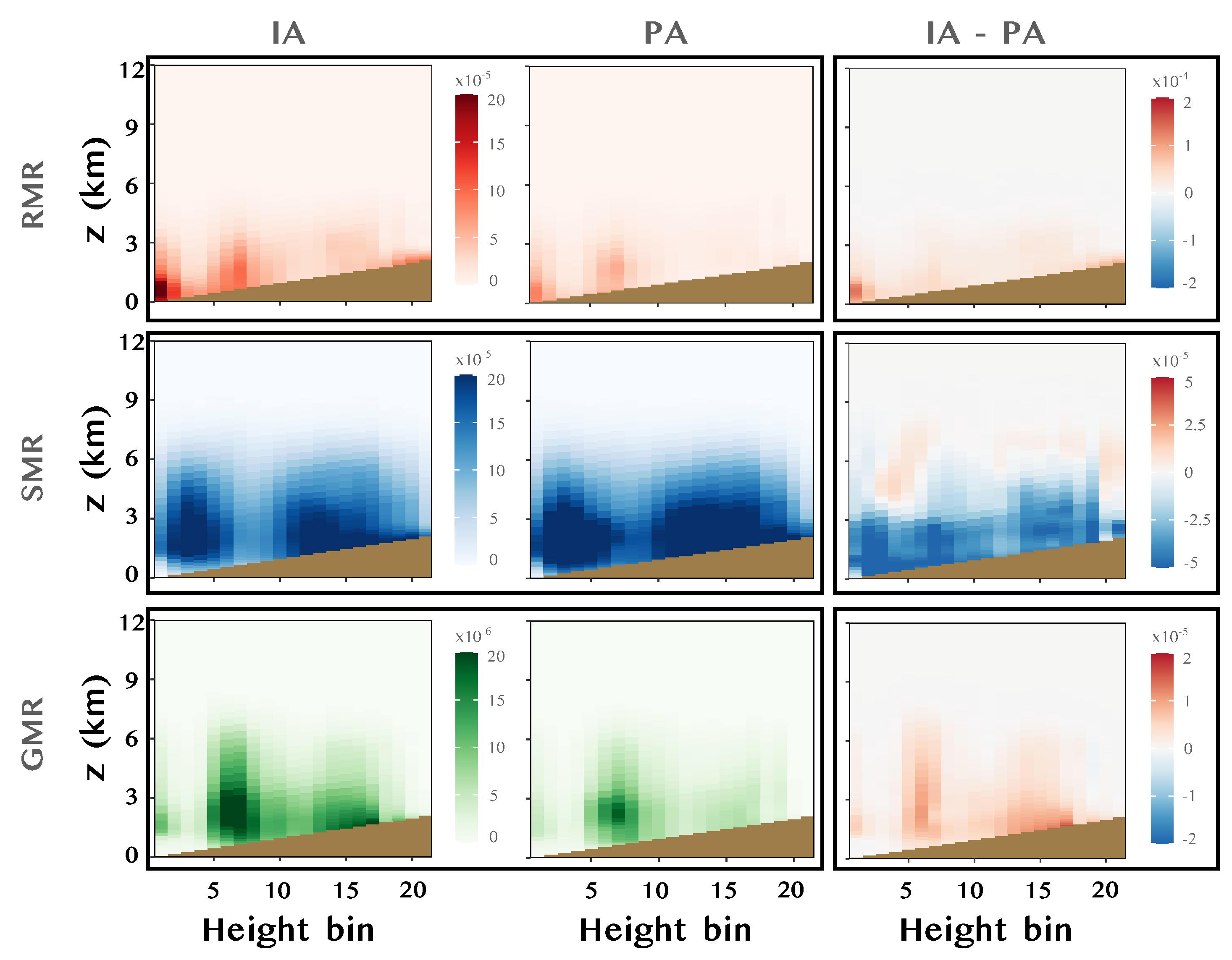
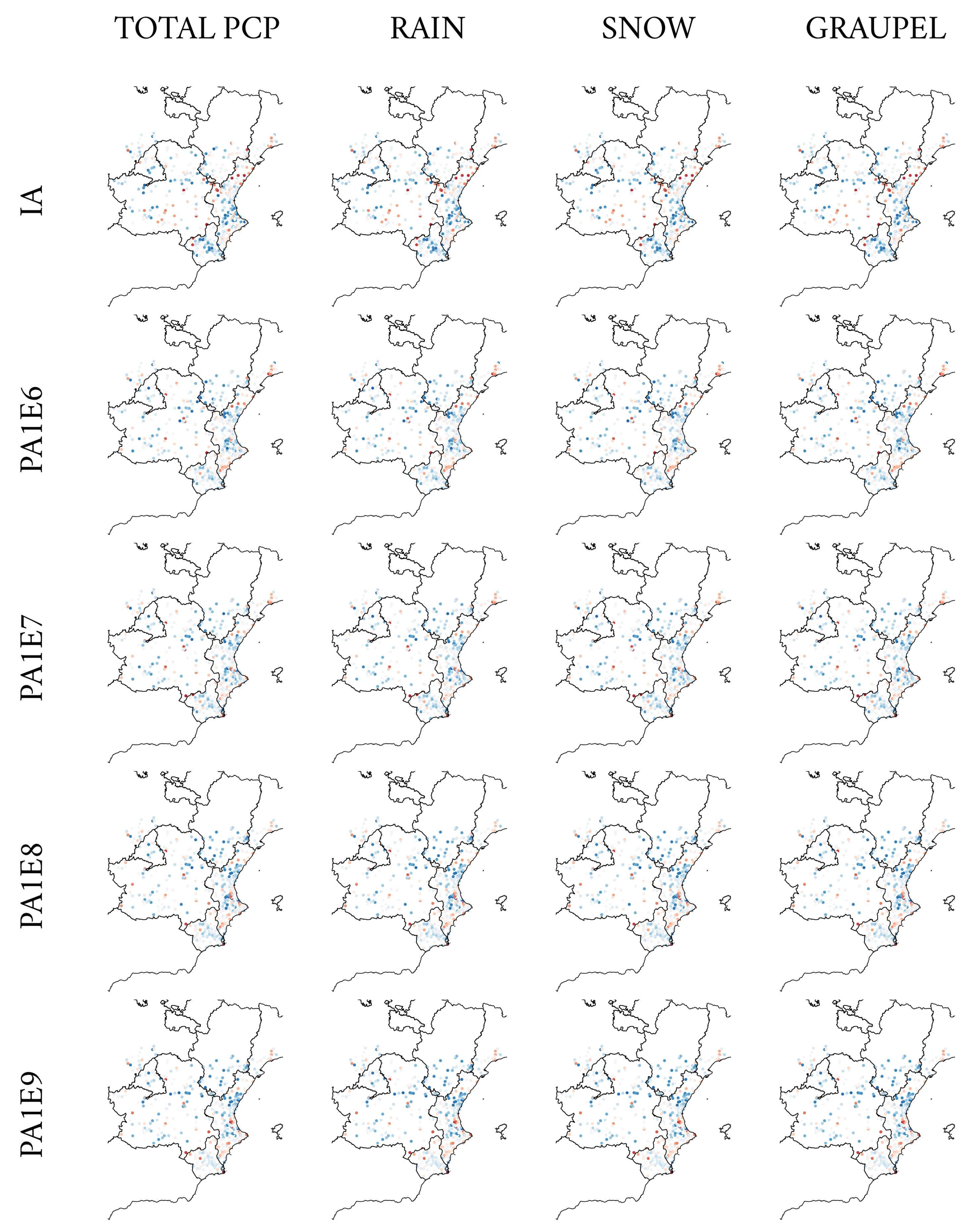
3.1. Effect of Interactive versus Prescribed Aerosols
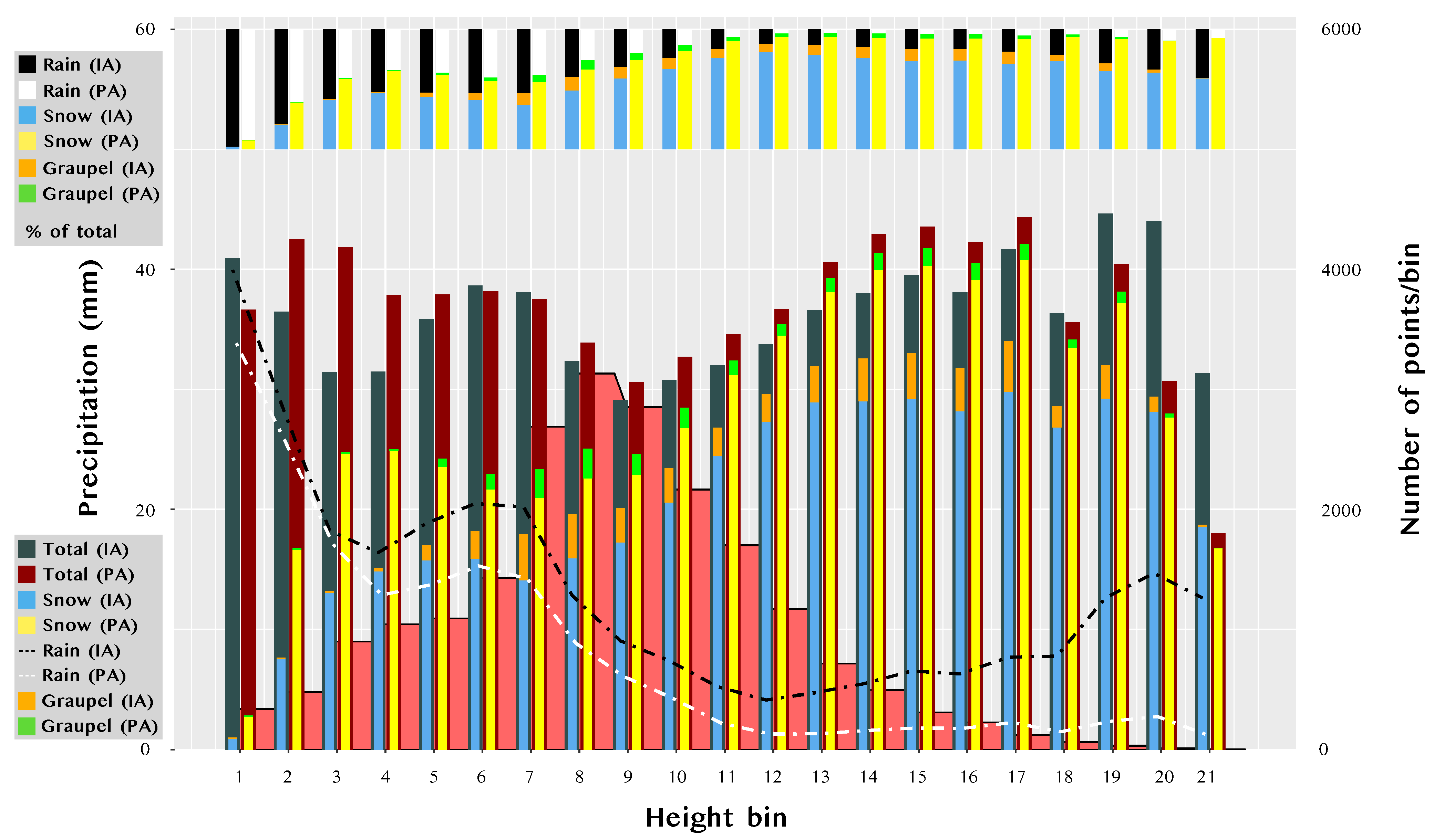
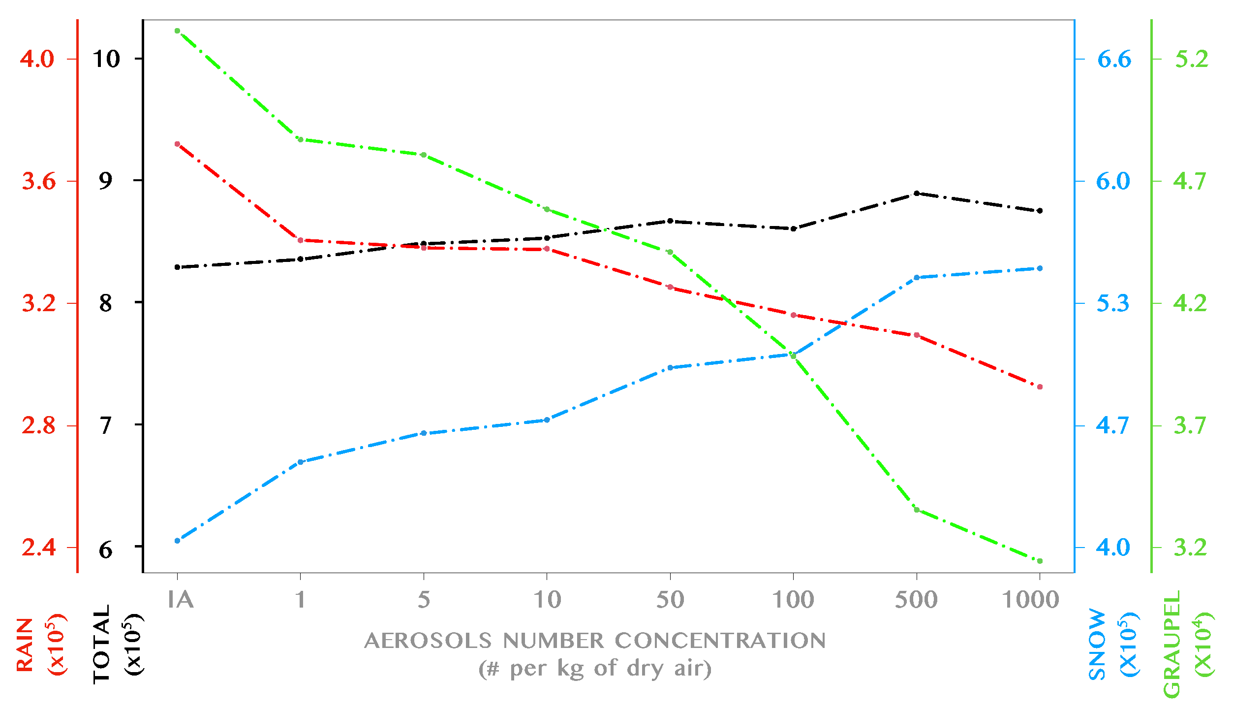
3.2. Sensitivity of Snow Formation Efficiency to the Number Concentration of Aerosols
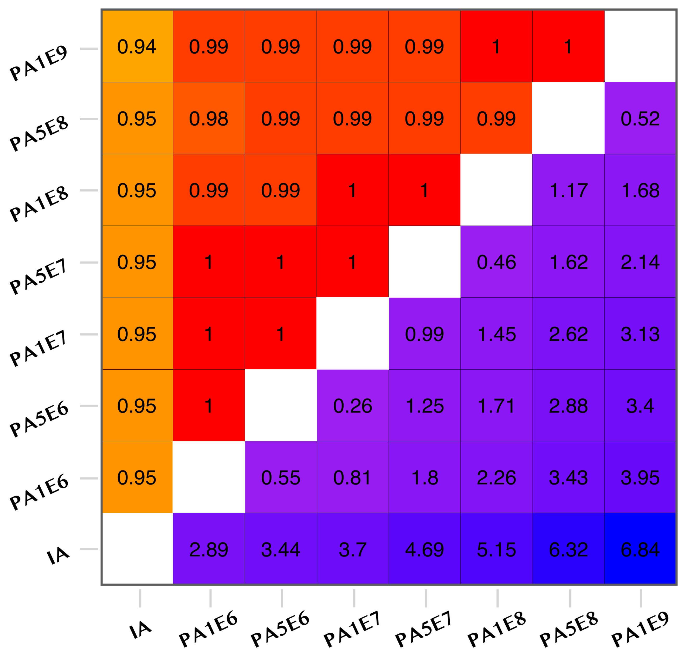
3.3. Evaluation of Simulations
4. Conclusions
Author Contributions
Funding
Data Availability Statement
Acknowledgments
Conflicts of Interest
Abbreviations
| PA | Prescribed Aerosols |
| IA | Intereactive Aerosols |
| CCN | Cloud Condensation Nuclei |
| LWC | Liquid Water Content |
| WBF | Wegener-Bergeron-Findeisen |
| WRF | Weather Research Forecast Model |
Appendix A

References
- Korolev, A.; McFarquhar, G.; Field, P.R.; Franklin, C.; Lawson, P.; Wang, Z.; Williams, E.; Abel, S.J.; Axisa, D.; Borrmann, S.; et al. Mixed-Phase Clouds: Progress and Challenges. Meteorol. Monogr. 2017, 58, 5.1–5.50. [Google Scholar] [CrossRef]
- Braham, R.R. Meteorological bases for precipitation development. Bull. Am. Meteorol. Soc. 1968, 49, 343–353. [Google Scholar] [CrossRef] [Green Version]
- Beard, K.V.; Ochs, H.T., III. Warm-rain initiation: An overview of microphysical mechanisms. J. Appl. Meteorol. Climatol. 1993, 32, 608–625. [Google Scholar] [CrossRef]
- Wegener, A. Thermodynamik der Atmosphäre; JA Barth: Leipzig, Germany, 1911. [Google Scholar]
- Bergeron, T. On the physics of clouds and precipitation. In Proceedings of the 5th Assembly UGGI, Lisbon, Portugal, 28 March 1935; pp. 156–180. [Google Scholar]
- Findeisen, W. Kolloid-meteorologische Vorgänge bei Neiderschlags-bildung. Meteor. Z. 1938, 55, 121–133. [Google Scholar]
- Twomey, S.; Squires, P. The influence of cloud nucleus population on the microstructure and stability of convective clouds. Tellus 1959, 11, 408–411. [Google Scholar] [CrossRef]
- Albrecht, B.A. Aerosols, Cloud Microphysics, and Fractional Cloudiness. Science 1989, 245, 1227–1230. [Google Scholar] [CrossRef]
- Bigg, E. The formation of atmospheric ice crystals by the freezing of droplets. Q. J. R. Meteorol. Soc. 1953, 79, 510–519. [Google Scholar] [CrossRef]
- Kanji, Z.A.; Ladino, L.A.; Wex, H.; Boose, Y.; Burkert-Kohn, M.; Cziczo, D.J.; Krämer, M. Overview of ice nucleating particles. Meteorol. Monogr. 2017, 58, 1.1–1.33. [Google Scholar] [CrossRef] [Green Version]
- Morrison, H.; van Lier-Walqui, M.; Fridlind, A.M.; Grabowski, W.W.; Harrington, J.Y.; Hoose, C.; Korolev, A.; Kumjian, M.R.; Milbrandt, J.A.; Pawlowska, H.; et al. Confronting the challenge of modeling cloud and precipitation microphysics. J. Adv. Model. Earth Syst. 2020, 12, e2019MS001689. [Google Scholar] [CrossRef]
- Reisin, T.; Levin, Z.; Tzivion, S. Rain production in convective clouds as simulated in an axisymmetric model with detailed microphysics. Part II: Effects of varying drops and ice initiation. J. Atmos. Sci. 1996, 53, 1815–1837. [Google Scholar] [CrossRef]
- Fan, J.; Leung, L.R.; Rosenfeld, D.; DeMott, P.J. Effects of cloud condensation nuclei and ice nucleating particles on precipitation processes and supercooled liquid in mixed-phase orographic clouds. Atmos. Chem. Phys. 2017, 17, 1017–1035. [Google Scholar] [CrossRef] [Green Version]
- Muhlbauer, A.; Hashino, T.; Xue, L.; Teller, A.; Lohmann, U.; Rasmussen, R.M.; Geresdi, I.; Pan, Z. Intercomparison of aerosol-cloud-precipitation interactions in stratiform orographic mixed-phase clouds. Atmos. Chem. Phys. 2010, 10, 8173–8196. [Google Scholar] [CrossRef] [Green Version]
- Borys, R.D.; Lowenthal, D.H.; Cohn, S.A.; Brown, W.O. Mountaintop and radar measurements of anthropogenic aerosol effects on snow growth and snowfall rate. Geophys. Res. Lett. 2003, 30, GL016855. [Google Scholar] [CrossRef]
- Xiao, H.; Yin, Y.; Chen, Q.; Zhao, P. Impact of aerosol and freezing level on orographic clouds: A sensitivity study. Atmos. Res. 2016, 176–177, 19–28. [Google Scholar] [CrossRef] [Green Version]
- Hallett, J.; Mossop, S. Production of secondary ice particles during the riming process. Nature 1974, 249, 26–28. [Google Scholar] [CrossRef]
- Reinking, R.F. Formation of graupel. J. Appl. Meteorol. 1975, 14, 745–754. [Google Scholar] [CrossRef]
- Scott, B.C.; Hobbs, P.V. A theoretical study of the evolution of mixed-phase cumulus clouds. J. Atmos. Sci. 1977, 34, 812–826. [Google Scholar] [CrossRef]
- Matsuo, T.; Mizuno, H.; Masataka, M.; Yoshinori, Y. Requisites of graupel formation in snow clouds over the sea of Japan. Atmos. Res. 1994, 32, 55–74. [Google Scholar] [CrossRef]
- Kumjian, M.R.; Ganson, S.M.; Ryzhkov, A.V. Freezing of raindrops in deep convective updrafts: A microphysical and polarimetric model. J. Atmos. Sci. 2012, 69, 3471–3490. [Google Scholar] [CrossRef]
- Sun, J.; Shi, Z.; Chai, J.; Xu, G.; Niu, B. Effects of mixed phase microphysical process on precipitation in a simulated convective cloud. Atmosphere 2016, 7, 97. [Google Scholar] [CrossRef] [Green Version]
- Thériault, J.M.; Stewart, R. On the effects of vertical air velocity on winter precipitation types. Nat. Hazards Earth Syst. Sci. 2007, 7, 231–242. [Google Scholar] [CrossRef] [Green Version]
- Ramelli, F.; Henneberger, J.; David, R.O.; Bühl, J.; Radenz, M.; Seifert, P.; Wieder, J.; Lauber, A.; Pasquier, J.T.; Engelmann, R.; et al. Microphysical investigation of the seeder and feeder region of an Alpine mixed-phase cloud. Atmos. Chem. Phys. 2021, 21, 6681–6706. [Google Scholar] [CrossRef]
- Khain, A. Notes on state-of-the-art investigations of aerosol effects on precipitation: A critical review. Environ. Res. Lett. 2009, 4, 015004. [Google Scholar] [CrossRef]
- Letcher, T.; Cotton, W.R. The effect of pollution aerosol on wintertime orographic precipitation in the Colorado Rockies using a simplified emissions scheme to predict CCN concentrations. J. Appl. Meteorol. Climatol. 2014, 53, 859–872. [Google Scholar] [CrossRef]
- Saleeby, S.M.; Cotton, W.R.; Lowenthal, D.; Messina, J. Aerosol impacts on the microphysical growth processes of orographic snowfall. J. Appl. Meteorol. Climatol. 2013, 52, 834–852. [Google Scholar] [CrossRef]
- Ilotoviz, E.; Khain, A.P.; Benmoshe, N.; Phillips, V.T.; Ryzhkov, A.V. Effect of aerosols on freezing drops, hail, and precipitation in a midlatitude storm. J. Atmos. Sci. 2016, 73, 109–144. [Google Scholar] [CrossRef]
- Agencia Estatal de Meteorología. Informe Sobre el Episodio Meteorológico de Fuertes Nevadas y Precipitaciones Ocasionadas por Borrasca Filomena y Posterior Ola de FríO. 2021. Available online: http://www.aemet.es/documentos/es/conocermas/recursos_en_linea/publicaciones_y_estudios/estudios/Informe_episodio_filomena.pdf (accessed on 11 November 2012).
- Grell, G.A.; Peckham, S.E.; Schmitz, R.; McKeen, S.A.; Frost, G.; Skamarock, W.C.; Eder, B. Fully coupled “online” chemistry within the WRF model. Atmos. Environ. 2005, 39, 6957–6975. [Google Scholar] [CrossRef]
- Skamarock, W.; Klemp, J.; Dudhia, J.; Gill, D.; Barker, D.; Wang, W.; Powers, J. A Description of the Advanced Research WRF Version 3; NCAR: Boulder, CO, USA, 2008; Volume 27, pp. 3–27. [Google Scholar]
- Mlawer, E.J.; Taubman, S.J.; Brown, P.D.; Iacono, M.J.; Clough, S.A. Radiative transfer for inhomogeneous atmospheres: RRTM, a validated correlated-k model for the longwave. J. Geophys. Res. Atmos. 1997, 102, 16663–16682. [Google Scholar] [CrossRef] [Green Version]
- Monin, A.S.; Obukhov, A.M. Basic laws of turbulent mixing in the surface layer of the atmosphere. Contrib. Geophys. Inst. Acad. Sci. USSR 1954, 151, e187. [Google Scholar]
- Jiménez, P.A.; Dudhia, J.; González-Rouco, J.F.; Navarro, J.; Montávez, J.P.; García-Bustamante, E. A Revised Scheme for the WRF Surface Layer Formulation. Mon. Weather Rev. 2012, 140, 898–918. [Google Scholar] [CrossRef] [Green Version]
- Mitchell, K. The Community Noah Land-Surface Model (LSM). User’s Guide. Recover. 2005; Volume 7. Available online: http://www.emc.ncep.noaa.gov/mmb/gcp/ldas/noahlsm/ver_2 (accessed on 20 July 2022).
- Hong, S.Y.; Noh, Y.; Dudhia, J. A new vertical diffusion package with an explicit treatment of entrainment processes. Mon. Weather Rev. 2006, 134, 2318–2341. [Google Scholar] [CrossRef] [Green Version]
- Jiménez, P.A.; Dudhia, J. Improving the representation of resolved and unresolved topographic effects on surface wind in the WRF model. J. Appl. Meteorol. Climatol. 2012, 51, 300–316. [Google Scholar] [CrossRef] [Green Version]
- Grell, G.A.; Dévényi, D. A generalized approach to parameterizing convection combining ensemble and data assimilation techniques. Geophys. Res. Lett. 2002, 29, 38-1–38-4. [Google Scholar] [CrossRef] [Green Version]
- Berrisford, P.; Dee, D.; Poli, P.; Brugge, R.; Fielding, M.; Fuentes, M.; Kållberg, P.; Kobayashi, S.; Uppala, S.; Simmons, A. The ERA-Interim Archive Version 2.0; ECMWF: Reading, UK, 2011; p. 23. [Google Scholar]
- Morrison, H.; Curry, J.; Khvorostyanov, V. A new double-moment microphysics parameterization for application in cloud and climate models. Part I: Description. J. Atmos. Sci. 2005, 62, 1665–1677. [Google Scholar] [CrossRef]
- Lim, K.S.S.; Hong, S.Y. Development of an effective double-moment cloud microphysics scheme with prognostic cloud condensation nuclei (CCN) for weather and climate models. Mon. Weather Rev. 2010, 138, 1587–1612. [Google Scholar] [CrossRef] [Green Version]
- Grabowski, W.W.; Morrison, H. Untangling microphysical impacts on deep convection applying a novel modeling methodology. Part II: Double-moment microphysics. J. Atmos. Sci. 2016, 73, 3749–3770. [Google Scholar] [CrossRef]
- Grabowski, W.W. Indirect impact of atmospheric aerosols in idealized simulations of convective–radiative quasi equilibrium. J. Clim. 2006, 19, 4664–4682. [Google Scholar] [CrossRef] [Green Version]
- Gettelman, A.; Morrison, H.; Santos, S.; Bogenschutz, P.; Caldwell, P. Advanced two-moment bulk microphysics for global models. Part II: Global model solutions and aerosol–cloud interactions. J. Clim. 2015, 28, 1288–1307. [Google Scholar] [CrossRef]
- Morrison, H.; Thompson, G.; Tatarskii, V. Impact of cloud microphysics on the development of trailing stratiform precipitation in a simulated squall line: Comparison of one-and two-moment schemes. Mon. Weather Rev. 2009, 137, 991–1007. [Google Scholar] [CrossRef] [Green Version]
- Chapman, E.G.; Gustafson, W.I., Jr.; Easter, R.C.; Barnard, J.C.; Ghan, S.J.; Pekour, M.S.; Fast, J.D. Coupling aerosol-cloud-radiative processes in the WRF-Chem model: Investigating the radiative impact of elevated point sources. Atmos. Chem. Phys. 2009, 9, 945–964. [Google Scholar] [CrossRef] [Green Version]
- Gustafson, W.I., Jr.; Chapman, E.G.; Ghan, S.J.; Easter, R.C.; Fast, J.D. Impact on modeled cloud characteristics due to simplified treatment of uniform cloud condensation nuclei during NEAQS 2004. Geophys. Res. Lett. 2007, 34, GL030021. [Google Scholar] [CrossRef]
- Morrison, H.; Grabowski, W.W. Comparison of Bulk and Bin Warm-Rain Microphysics Models Using a Kinematic Framework. J. Atmos. Sci. 2007, 64, 2839–2861. [Google Scholar] [CrossRef] [Green Version]
- Petters, M.D.; Kreidenweis, S.M. A single parameter representation of hygroscopic growth and cloud condensation nucleus activity. Atmos. Chem. Phys. 2007, 7, 1961–1971. [Google Scholar] [CrossRef] [Green Version]
- Wang, Y.; Fan, J.; Zhang, R.; Leung, L.R.; Franklin, C. Improving bulk microphysics parameterizations in simulations of aerosol effects. J. Geophys. Res. Atmos. 2013, 118, 5361–5379. [Google Scholar] [CrossRef]
- Abdul-Razzak, H.; Ghan, S.J. A parameterization of aerosol activation: 2. Multiple aerosol types. J. Geophys. Res. Atmos. 2000, 105, 6837–6844. [Google Scholar] [CrossRef]
- Chin, M.; Rood, R.B.; Lin, S.J.; Müller, J.F.; Thompson, A.M. Atmospheric sulfur cycle simulated in the global model GOCART: Model description and global properties. J. Geophys. Res. Atmos. 2000, 105, 24671–24687. [Google Scholar] [CrossRef]
- Hoarau, T.; Barthe, C.; Tulet, P.; Claeys, M.; Pinty, J.P.; Bousquet, O.; Delanoë, J.; Vié, B. Impact of the generation and activation of sea salt aerosols on the evolution of Tropical Cyclone Dumile. J. Geophys. Res. Atmos. 2018, 123, 8813–8831. [Google Scholar] [CrossRef]
- Gong, S.L. A parameterization of sea-salt aerosol source function for sub- and super-micron particles. Glob. Biogeochem. Cycles 2003, 17, 2079. [Google Scholar] [CrossRef]
- Bian, H.; Froyd, K.; Murphy, D.M.; Dibb, J.; Darmenov, A.; Chin, M.; Colarco, P.R.; da Silva, A.; Kucsera, T.L.; Schill, G.; et al. Observationally constrained analysis of sea salt aerosol in the marine atmosphere. Atmos. Chem. Phys. 2019, 19, 10773–10785. [Google Scholar] [CrossRef] [Green Version]
- Gerber, H.E. Relative-Humidity Parameterization of the Navy Aerosol Model (NAM); Technical Report; Naval Research Lab: Washington, DC, USA, 1985. [Google Scholar]
- Chin, M.; Ginoux, P.; Kinne, S.; Torres, O.; Holben, B.N.; Duncan, B.N.; Martin, R.V.; Logan, J.A.; Higurashi, A.; Nakajima, T. Tropospheric aerosol optical thickness from the GOCART model and comparisons with satellite and Sun photometer measurements. J. Atmos. Sci. 2002, 59, 461–483. [Google Scholar] [CrossRef]
- Yahya, K.; Glotfelty, T.; Wang, K.; Zhang, Y.; Nenes, A. Modeling regional air quality and climate: Improving organic aerosol and aerosol activation processes in WRF/Chem version 3.7.1. Geosci. Model Dev. 2017, 10, 2333–2363. [Google Scholar] [CrossRef] [Green Version]
- Morrison, H.; Gettelman, A. A New Two-Moment Bulk Stratiform Cloud Microphysics Scheme in the Community Atmosphere Model, Version 3 (CAM3). Part I: Description and Numerical Tests. J. Clim. 2008, 21, 3642–3659. [Google Scholar] [CrossRef]
- Cooper, W.A. Ice Initiation in Natural Clouds. In Precipitation Enhancement—A Scientific Challenge; American Meteorological Society: Boston, MA, USA, 1986; pp. 29–32. [Google Scholar] [CrossRef]
- Morrison, H.; Milbrandt, J.A. Parameterization of Cloud Microphysics Based on the Prediction of Bulk Ice Particle Properties. Part I: Scheme Description and Idealized Tests. J. Atmos. Sci. 2015, 72, 287–311. [Google Scholar] [CrossRef]
- Pravia-Sarabia, E.; Halifa-Marín, A.; Gómez-Navarro, J.J.; Palacios-Peña, L.; Jiménez-Guerrero, P.; Montávez, J.P. On the role of aerosols in the production of orographically-induced extreme rainfall in near-maritime environments. Atmos. Res. 2022, 268, 106001. [Google Scholar] [CrossRef]
- Cooke, W.; Liousse, C.; Cachier, H.; Feichter, J. Construction of a 1° × 1° fossil fuel emission data set for carbonaceous aerosol and implementation and radiative impact in the ECHAM4 model. J. Geophys. Res. Atmos. 1999, 104, 22137–22162. [Google Scholar] [CrossRef]
- Murray, B.; O’sullivan, D.; Atkinson, J.; Webb, M. Ice nucleation by particles immersed in supercooled cloud droplets. Chem. Soc. Rev. 2012, 41, 6519–6554. [Google Scholar] [CrossRef] [Green Version]


| Sim | T | |||||||||||
|---|---|---|---|---|---|---|---|---|---|---|---|---|
| IA | [0–5] | 255.7 | 2154.6 | 2.4 (2) | 0.002 (9) | 4.7 (1) | 0.01 (7) | 32.0 | 0.02 (25) | 28.3 | 85.7 | 6.1 |
| PA1E6 | 1 | 255.8 | 2169.6 | 2.4 (6) | 0.003 (0) | 4.6 (9) | 0.02 (4) | 29.0 | 0.02 (25) | 26.5 | 91.0 | 5.3 |
| PA5E6 | 5 | 255.8 | 2174.0 | 3.3 | 0.004 (0) | 4.7 (2) | 0.07 (6) | 21.7 | 0.02 (27) | 25.2 | 93.5 | 5.3 |
| PA1E7 | 10 | 255.8 | 2172.4 | 4.0 | 0.004 (8) | 4.7 (1) | 0.14 (7) | 18.6 | 0.02 (25) | 24.2 | 94.6 | 5.1 |
| PA5E7 | 50 | 255.8 | 2170.8 | 6.4 | 0.007 (8) | 4.7 (3) | 0.70 (3) | 13.0 | 0.02 (29) | 20.8 | 98.4 (8) | 4.9 |
| PA1E8 | 100 | 255.8 | 2171.1 | 7.6 | 0.009 (3) | 4.6 (8) | 1.31 (1) | 11.1 | 0.02 (26) | 18.7 | 98.5 (5) | 4.5 |
| PA5E8 | 500 | 255.8 | 2175.4 | 10.6 | 0.013 (0) | 4.7 (5) | 4.85 (2) | 8.1 | 0.02 (32) | 15.4 | 105.1 | 3.9 |
| PA1E9 | 1000 | 255.8 | 2169.7 | 11.6 | 0.014 (2) | 4.6 (9) | 7.75 (5) | 7.1 | 0.02 (30) | 14.0 | 105.6 | 3.7 |
| Sim | T | |||||||||||
|---|---|---|---|---|---|---|---|---|---|---|---|---|
| IA | [0–5] | 285.6 | 9171.6 | 563.8 | 0.6 (9) | 180.2 | 3.8 (7) | 32.6 | 0.7 (12) | 3524.1 | 2676.9 | 3024.1 |
| PA1E6 | 1 | 285.2 | 8855.2 | 573.1 | 0.7 (0) | 164.1 | 3.9 (4) | 32.6 | 0.7 (05) | 2919.4 | 2789.9 | 2366.0 |
| PA5E6 | 5 | 285.2 | 8902.1 | 633.5 | 0.7 (7) | 160.8 | 5.0 | 31.2 | 0.7 (00) | 2582.2 | 3631.5 | 2156.0 |
| PA1E7 | 10 | 285.2 | 8878.1 | 754.5 | 0.9 (2) | 167.2 | 10.0 | 26.2 | 0.7 (12) | 2867.8 | 2890.8 | 1969.6 |
| PA5E7 | 50 | 285.5 | 8965.0 | 911.6 | 1.1 (2) | 162.7 | 49.9 | 16.3 | 0.7 (06) | 2201.5 | 3558.2 | 2549.4 |
| PA1E8 | 100 | 285.5 | 8959.1 | 925.0 | 1.1 (3) | 167.3 | 99.6 | 13.1 | 0.7 (01) | 2159.2 | 3294.0 | 2186.0 |
| PA5E8 | 500 | 285.9 | 9160.6 | 1163.5 | 1.4 (3) | 178.7 | 498.4 | 8.2 | 0.7 (06) | 1986.8 | 3440.6 | 2454.6 |
| PA1E9 | 1000 | 285.5 | 8873.7 | 1321.8 | 1.6 (2) | 163.2 | 993.5 | 6.8 | 0.7 (09) | 2179.9 | 3320.4 | 2076.9 |
| Sim | PTCP RM | RAIN RM | SNOW RM | TPCP CR | RAIN CR | SNOW CR | TPCP BS | RAIN BS | SNOW BS |
|---|---|---|---|---|---|---|---|---|---|
| IA | 17.99 | 17.81 | 15.29 | 0.64 | 0.78 | 0.66 | 5.01 | 9.26 | −4.70 |
| PA1E6 | 16.11 | 15.34 | 15.07 | 0.67 | 0.79 | 0.66 | 4.03 | 6.42 | −2.82 |
| PA5E6 | 16.31 | 15.25 | 15.24 | 0.66 | 0.79 | 0.66 | 4.60 | 6.41 | −2.21 |
| PA1E7 | 16.45 | 15.33 | 15.28 | 0.65 | 0.78 | 0.66 | 4.69 | 6.43 | −2.08 |
| PA5E7 | 16.39 | 14.72 | 15.32 | 0.65 | 0.79 | 0.66 | 4.67 | 5.75 | −1.33 |
| PA1E8 | 16.59 | 14.49 | 15.39 | 0.63 | 0.79 | 0.66 | 4.32 | 5.02 | −0.80 |
| PA5E8 | 17.13 | 14.25 | 15.75 | 0.61 | 0.78 | 0.67 | 5.08 | 4.37 | 0.90 |
| PA1E9 | 16.70 | 13.74 | 15.51 | 0.61 | 0.79 | 0.68 | 4.27 | 3.42 | 1.08 |
| Sim | TPCP RM | RAIN RM | SNOW RM | TPCP CR | RAIN CR | SNOW CR | TPCP BS | RAIN BS | SNOW BS |
|---|---|---|---|---|---|---|---|---|---|
| IA | 11.16 | 12.13 | 13.09 | 0.83 | 0.88 | 0.77 | 2.51 | 5.86 | −3.97 |
| PA1E6 | 10.02 | 10.68 | 12.53 | 0.86 | 0.89 | 0.78 | 2.01 | 4.07 | −2.64 |
| PA5E6 | 10.43 | 10.74 | 12.58 | 0.85 | 0.89 | 0.77 | 2.54 | 4.11 | −2.14 |
| PA1E7 | 10.43 | 10.62 | 12.51 | 0.85 | 0.89 | 0.77 | 2.61 | 4.10 | −2.02 |
| PA5E7 | 11.23 | 10.67 | 12.40 | 0.82 | 0.89 | 0.78 | 2.70 | 3.61 | −1.42 |
| PA1E8 | 11.70 | 10.46 | 12.28 | 0.80 | 0.89 | 0.78 | 2.62 | 3.12 | −0.99 |
| PA5E8 | 12.53 | 10.37 | 12.35 | 0.77 | 0.89 | 0.79 | 3.14 | 2.67 | 0.26 |
| PA1E9 | 12.32 | 10.12 | 12.17 | 0.77 | 0.89 | 0.79 | 2.55 | 1.97 | 0.49 |
Disclaimer/Publisher’s Note: The statements, opinions and data contained in all publications are solely those of the individual author(s) and contributor(s) and not of MDPI and/or the editor(s). MDPI and/or the editor(s) disclaim responsibility for any injury to people or property resulting from any ideas, methods, instructions or products referred to in the content. |
© 2023 by the authors. Licensee MDPI, Basel, Switzerland. This article is an open access article distributed under the terms and conditions of the Creative Commons Attribution (CC BY) license (https://creativecommons.org/licenses/by/4.0/).
Share and Cite
Pravia-Sarabia, E.; Montávez, J.P.; Halifa-Marin, A.; Jiménez-Guerrero, P.; Gomez-Navarro, J.J. The Role of Aerosol Concentration on Precipitation in a Winter Extreme Mixed-Phase System: The Case of Storm Filomena. Remote Sens. 2023, 15, 1398. https://doi.org/10.3390/rs15051398
Pravia-Sarabia E, Montávez JP, Halifa-Marin A, Jiménez-Guerrero P, Gomez-Navarro JJ. The Role of Aerosol Concentration on Precipitation in a Winter Extreme Mixed-Phase System: The Case of Storm Filomena. Remote Sensing. 2023; 15(5):1398. https://doi.org/10.3390/rs15051398
Chicago/Turabian StylePravia-Sarabia, Enrique, Juan Pedro Montávez, Amar Halifa-Marin, Pedro Jiménez-Guerrero, and Juan José Gomez-Navarro. 2023. "The Role of Aerosol Concentration on Precipitation in a Winter Extreme Mixed-Phase System: The Case of Storm Filomena" Remote Sensing 15, no. 5: 1398. https://doi.org/10.3390/rs15051398