1. Introduction
As an important part of the earth system, Antarctica’s ice sheet not only plays an important role in the study of surface heat balance, atmospheric circulation, sea level rise and fall, ocean physics, and biogeochemical cycles but also stores a large amount of information reflecting the global climate and ecological environment changes [
1].
As one of the basic characteristic parameters of an ice sheet, accurate snow temperature profiles above the ice sheet is not only a boundary condition for establishing an ice sheet dynamics model and estimating ice sheet mass balance but also an important variable for studying ice sheet isostatic adjustment, ice sheet dynamics [
2], and global sea level change [
3].
Up to now, the snow temperature profiles are usually obtained in situ in a limited number of boreholes [
4,
5], which can be very accurate, but the samples are too sparse to represent the whole continent. Remote sensing of snow temperature by spaceborne radiometers was limited to the snow surface or at a single depth by using thermal infrared sensors [
6] and microwave passive sensors [
7]. Processed MODIS snow surface temperature data were compared with in situ hourly measurements of surface temperature data with a bias ranging from −1.8 °C to 0.1 °C, and root mean square error ranging from 2.2 °C to 4.8 °C in Freville’s research [
6]. Brogioni used the microwave BT at 19 GHz and 37 GHz to invert the snow temperature at 1 m depth, with RMSE around 1 K [
7].
The snow surface temperature can be inverted from infrared BT or microwave BT. Combining infrared BT and microwave BT to invert snow surface temperature is helpful in improving the accuracy of snow surface temperature. Meanwhile, microwaves with different frequencies have different penetration depths in snow, indicating that the microwave brightness temperature (BT) contains information on snow temperature at different depths. Thus, it is better to invert the snow temperature profiles by combining multi-frequency microwave BT and infrared BT.
This paper proposes a conjoint inversion algorithm to invert snow temperature profiles by combining microwave BT from AMSR2 with infrared BT from MODIS. The MODIS BT data are weighted by microwave antenna pattern, while the weight functions are applied to the AMSR2 BT data, and the atmospheric correction is also taken into consideration. The results are evaluated by comparing them with the measured snow temperature at Dome-C station in 2017 and 2018.
The paper is structured as follows.
Section 2 provides the data sources used in this study.
Section 3 describes the methodology used for snow temperature profile inversion.
Section 4 and
Section 5 are devoted to the presentation of the obtained results and to their discussion, respectively. Finally,
Section 6 presents the main conclusions of the study.
2. Data
The input data are microwave and infrared data. We choose the input data from AMSR2 and MODIS to reduce the influence of time-space mismatch because the satellites GCOM-W1 (equipped with the microwave radiometer, AMSR2) and Aqua (equipped with the infrared radiometer, MODIS) are in parallel operation (both belong to A-Train) [
8]. The verification data of snow temperature profiles are obtained from Dome-C scientific station.
2.1. Input Data
2.1.1. AMSR2 Data
The AMSR2 BT data are provided by the G-Portal website (
https://gportal.jaxa.jp, accessed on 28 April 2022), including the channels of 6.93 GHz, 10.63 GHz, 18.7 GHz, 23.8 GHz, 36.5 GHz, and 89.0 GHz with both V and H polarization. AMSR2 was launched on GCOM-W1 in May 2012 with the main mission of monitoring the global water cycle [
8].
Table 1 shows the frequency, polarization, and spatial resolution of the channels. Because the 6.93 GHz brightness temperature is essential for remote sensing of snow temperature in deep layers, the BT data of all channels need to be processed by quality control, resampled, and matched to the resolution of the 6.93 GHz channel. The processed BT can be obtained from the L1 R brightness temperature provided by the G-Portal website.
2.2. Verification Data
The data observed at Dome-C scientific station are used to assess the accuracy of the inverted snow temperature profiles. The snow temperature profiles are recorded every hour by Dome-C scientific station (
http://www.climantartide.it, accessed on 22 April 2022). Dome-C scientific station was established jointly by Italy and France. The Dome-C scientific station is located in the middle of the East Antarctic plateau (75.1°S, 123.35°E). This website provides snow temperature data for 5 cm, 10 cm, 25 cm, 50 cm, 100 cm, 150 cm, 200 cm, 250 cm, 300 cm, 400 cm, 500 cm, and 1000 cm depths under the snow at Dome-C scientific station.
3. Methods
This paper proposes a conjoint inversion algorithm to retrieve snow temperature profiles by combining multi-frequency microwave BT with infrared BT.
Figure 1 shows the differences in penetration depth and spatial resolution between microwave and infrared remote sensing for snow temperature profiles and shows that atmospheric factors cannot be ignored. Thus, the conjoint inversion algorithm takes the following aspects into consideration.
The infrared BT and the microwave BT received from space are both affected by the atmosphere. In order to accurately invert snow temperature profiles, it is necessary to adopt atmospheric correction for microwave BT and infrared BT.
Considering that infrared and microwaves at different frequencies have different penetration depths in snow, the snow temperature profiles can be retrieved by combining multi-frequency microwave and infrared BT. The weight functions of microwave BT at different frequencies are applied because the penetration depths in snow are different at different frequencies.
Considering that the spatial resolution of infrared is higher than that of microwaves, the infrared BT data are synthesized in each microwave footprint by the normalized microwave antenna pattern weighting method to match the microwave and infrared BT data in the footprint [
11].
Section 3.2 analyzes the relationship between brightness temperature and snow temperature. Based on the analysis, the conjoint inversion algorithm is proposed in
Section 3.3, and inversion steps are shown in
Section 3.4.
3.1. Atmospheric Correction
According to the radiation transfer theory, the BT that the spaceborne infrared radiometers receive is affected by atmospheric scattering. Meanwhile, BT received by the spaceborne microwave radiometers is partially absorbed by the atmosphere. Different atmospheric correction methods are used for microwave and infrared. The influence of the atmosphere is eliminated in infrared surface temperature inversion by comparing absorption property differences of 10.4~12.9 μm thermal infrared band [
12].
Based on the radiation transfer model, atmospheric correction is adopted for the microwave BT [
13]:
where
is the BT received by a microwave radiometer, which is called the top atmosphere BT;
is the atmospheric transmissivity;
is the surface BT;
and
are the upwelling atmospheric BT and the downwelling atmospheric BT, respectively;
is the surface reflectivity;
is the brightness temperature from snow, and
is the cold space BT.
,
, and
are calculated as follows [
13]:
where
represents the absorption coefficient of the atmosphere which can be calculated by the water vapor and air temperature according to Wentz’s work [
14]; TOA means the top of the atmosphere;
represents air temperature at z (m) above the surface. The air temperature and water vapor profile data used to calculate atmospheric parameters are from MODIS.
The snow BT can be obtained by:
3.2. Analysis of the Relationship between Brightness Temperature and Snow Temperature
In order to determine the brightness temperature combination form of the inversion algorithm, the variation trend of brightness temperature with snow temperature should be analyzed. In this section, we will analyze the relationship between snow temperature and infrared BT and microwave BT, respectively.
For infrared remote sensing of snow temperature, the penetration depth into snow is extremely thin at a depth of ~20 μm. The infrared brightness temperature on the snow surface can be expressed as:
where
is snow emissivity of infrared,
is the snow surface temperature. According to Equation (7), the snow temperature on the surface is linearly correlated with the infrared brightness temperature.
For microwave remote sensing of snow temperature, the brightness temperature of snow
can be expressed as:
where
is snow emissivity of microwave channel
i, which mainly depends on the snow grain size and the snow density [
15].
is the absorption coefficient and scattering coefficient in snow, which is related to the frequencies of microwaves, so microwaves at different frequencies have different penetration depths in the snow.
is the incidence angle,
is the snow temperature profile, and z is the vertical depth of the snow. If the snow is divided into
layers of thickness
, Equation (8) can be written as Equation (9). Because the change of the emissivity at a given location with time is negligible [
16], according to Equation (9), the snow microwave BT has a linear relationship with the snow temperature.
The microwave BT is related to the snow temperature profile and penetration depth, and microwaves at different frequencies have different penetration depths; thus, the variation amplitude of microwave BT at different frequencies caused by the change of snow temperature at different depths is also different.
The brightness temperature change
caused by two different snow temperature profiles
and
is:
where
represents the BT change of microwave channel
i when the snow temperature profile changes from
to
. Therefore, we can analyze the variation amplitude of the brightness temperature of different frequencies due to the snow temperature variation at different depths.
When inverting snow temperature by linear combination of microwave BT, microwave BT can be weighted, and the weight functions can be expressed as:
Considering the linear relationship between BT and snow temperature, the microwave BT and the infrared BT data are linearly combined in the conjoint inversion algorithm, while the different weight functions of microwave BT at different frequencies are applied because the penetration depths in snow are different at different frequencies.
3.3. Conjoint Inversion Algorithm of Snow Temperature Profiles
The conjoint inversion algorithm is derived by linear combination of infrared BT and weighted microwave BT and considering atmospheric correction:
where
is the snow temperature at
(m) depth;
is regression coefficient;
is the infrared term;
is the microwave term.
The infrared term
uses the form of surface temperature algorithm [
10,
12,
17]:
where
are regression coefficients;
is the zenith angle;
and
are the synthesis infrared BT at 11 μm and 12 μm. The synthesis infrared BT is the integral of infrared BT weighted by microwave antenna pattern [
11].
.
is used for atmospheric correction.
are obtained from Equation (15):
where
and
are the infrared BT at 11 μm and 12 μm respectively;
represents the normalized microwave antenna pattern corresponding to the specific observation. F refers to the coverage of infrared data within the microwave footprint [
11].
The microwave term
can be expressed as:
where
and
are the regression coefficient;
are weight functions from Equation (12); subscript
of
and
means the channel
i of AMSR2 (see
Table 1).
is the BT above the snow surface, which can be obtained from Equation (6).
is the auxiliary term for atmospheric correction of the corresponding frequency band.
The conjoint inversion algorithm is also applicable to the inversion of snow temperature separately from microwave or infrared. When there are no infrared BT data, microwave BT data can be used to invert snow temperature profiles with Equation (13), in which is set to 0. When there are no microwave BT data, the snow surface temperature data can be inverted from infrared BT data with set to 0 in Equation (13).
3.4. Inversion Steps
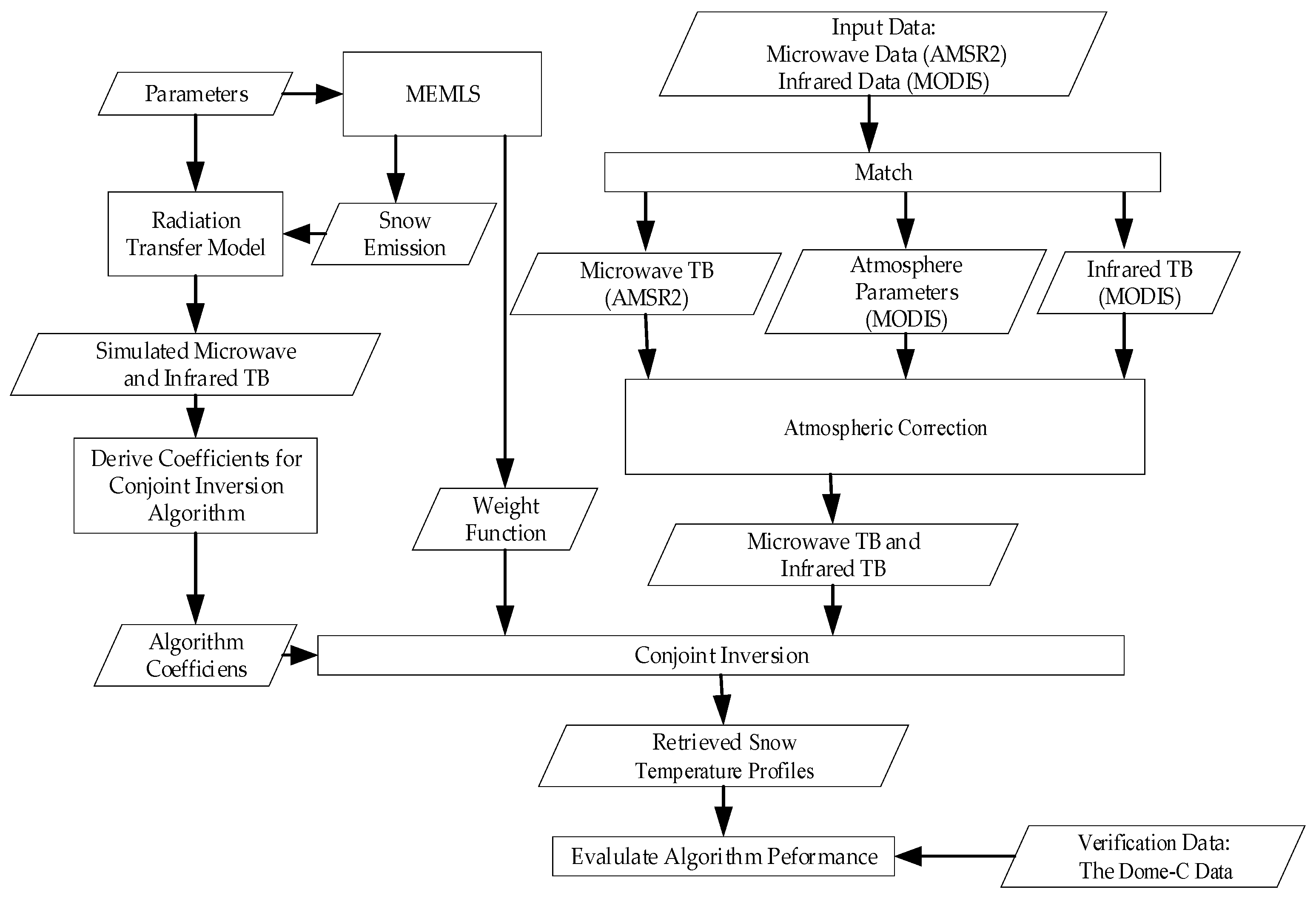
Figure 2 shows the inversion steps of snow temperature profiles.
For the emission of snow, because the wavelength of microwave frequency in 5~100 GHz is close to snow particle size, the scattering effect caused by snow grain can not be ignored. A number of snow emission radiative transfer models have been developed based on a range of theoretical assumptions [
18,
19,
20]. Pan compares the basic theories of two models: the multiplayer Helsinki University of Technology (HUT) model [
19] and the microwave emission model of layered snowpacks (MEMLS) [
18,
21], and finds that MEMLS performs better [
22]. Wiesmann and Mätzler have developed the MEMLS based on radiative transfer, using the six-flux theory to describe multiple volume scattering and absorption, including radiation trapping due to internal reflection and a combination of coherent and incoherent superposition of reflections between layer interfaces [
18,
21]. The input parameters of MEMLS include frequency (GHz), incidence angle (°), snow temperature profile (°C), snow correlation length profile (mm) (can be calculated by snow grain size profile [
23]), and snow density profile (kg/m
3).
The specific inversion steps are as follows.
The parameters of snow density and snow grain size required for MEMLS calculation of brightness temperature come from the Dome-C station. Microwave frequencies are set to 6.93 GHz, 10.65 GHz, 18.7 GHz, 23.8 GHz, 36.5 GHz, and 89.0 GHz, according to the AMSR2 parameters. The incidence angle is set to 55.3°. The snow temperature profile was obtained from Dome-C station at 0 UCT on 1 January 2017. Snow grain size profiles are obtained from Macelloni’s work [
24]. Measurements showed that the density fluctuations are larger near the surface and tend to disappear as a function of depth [
16]. The average snow density profile used in this paper is from [
25]:
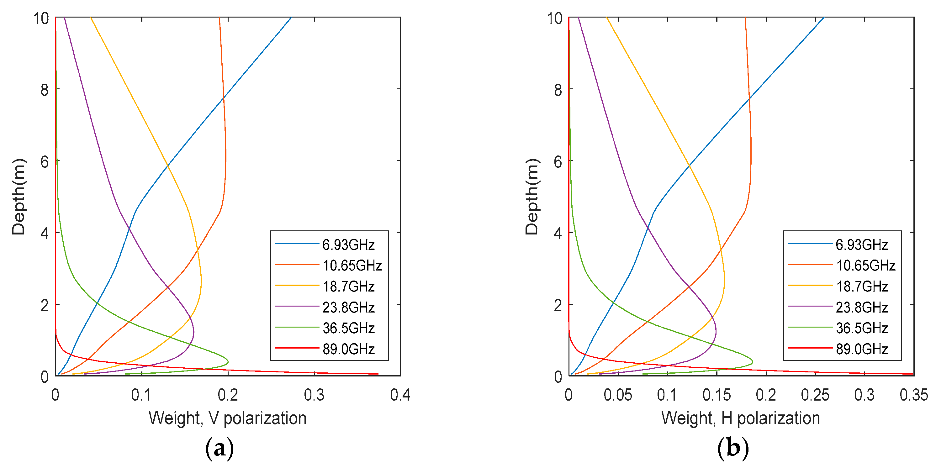
Then, the weight functions
can be calculated by Equation (12).
Figure 3 shows the weight of microwave BT at different frequencies.
- 2.
Based on the observed snow density and snow grain size at Dome-C station, we set up a scenario where snow temperature at different depths is randomly varied from −80 °C to −10 °C. About 40,000 scenes are generated in this manner. The microwave and infrared BT calculated from the theory of radiative transfer model are used as the input data to fit the parameters of Equation (13), and the coefficients are determined.
- 3.
We match the AMSR2 BT data, MODIS BT data, MODIS air temperature profile data, and MODIS water vapor profile data from 1 January 2017 to 31 December 2018 within the microwave footprint corresponding to the specific observation in space and 1 h in time. The normalized microwave antenna pattern is obtained from 6.93 GHz antenna pattern of AMSR2.
- 4.
Based on the atmospheric parameters provided by MODIS, atmospheric correction is applied to AMSR2 microwave BT.
- 5.
The snow temperature profile data are obtained by inversion according to Equation (13), and the data observed at the Dome-C station are used as the validation data to evaluate the accuracy.
When there are no infrared BT data, microwave BT data can be used to invert snow temperature profiles through inversion steps 1, 2, 4, and 5 with is set to 0 in Equation (13). When there are no microwave BT data, infrared BT data can be used to invert snow surface temperature through inversion steps 1, 2, and 5 with set to 0 in Equation (13).
4. Results and Analysis
In this section, the snow temperature profiles are retrieved from AMSR2 data and MODIS data, whereas the data measured at Dome-C station from 1 January 2017 to 31 December 2018 are used as a comparison reference to evaluate the accuracy of the snow temperature profiles inverted by the conjoint inversion algorithm.
4.1. Results
The area with the relatively uniform spatial distribution of snow grain size and snow density has been chosen for the inversion of the snow temperature profiles. This area is around Dome-C station (74.125°S~76.125°S; 119.125°E~126.125°E; about 222 km × 201 km).
The conjoint inverted snow temperature profile data near the Dome-C station on 1 April 2017 are shown in
Figure 4, in which the pentagram is the location of the Dome-C station.
Figure 4a shows the snow surface temperature in this area, and
Figure 4b shows the snow temperature profile from the snow surface to 10 m depth between 74.125°S and 76.125°S at 123.35°E.
4.2. Comparison and Verification
The data observed at Dome-C station are used to verify the conjoint inverted snow temperature profile data. In total, 2756 sets of data were matched in the years 2017 and 2018, which are used for verification.
Figure 5 presents the comparison between the conjoint inverted snow temperature curve and the observed data at Dome-C station over time at depths of 0.05 m, 0.5 m, and 10 m from 2017 to 2018.
Figure 6 presents the comparison between the conjoint inverted snow temperature profiles and the observed data at Dome-C station at 6:00 on 1 March, 6:00 on 1 June 6:00 on 5 September, and 8:00 on 1 December 2017, representing the four seasons.
Figure 7 presents the temperature difference (
) between the conjoint inverted snow temperature profiles and the observed data at the Dome-C station. The conjoint inverted snow temperature profiles can well reflect the trend of snow temperature change with time and depth.
As seen in
Figure 5,
Figure 6 and
Figure 7, the fluctuations of the conjoint inverted snow temperature profiles are larger near the snow surface and substantially decrease with depth, which is consistent with the snow temperature profile measured at Dome-C station.
Figure 8 presents the frequency histogram of the temperature difference (
) between the conjoint inverted snow temperature profiles and observed data at 0.05 m, 1.5 m, and 10 m depths, respectively. The figure shows the temperature difference at different depths is normally distributed.
The conjoint inverted snow temperature profile data are compared with the observed data from the Dome-C station. Due to the small annual variation of snow temperature in the deep layer, we add the relative accuracy parameter to assess the accuracy of the conjoint inverted snow temperature profiles in addition to the mean bias and standard deviation. The relative accuracy is defined by the following formula:
where
is the standard deviation of the results at
z (m) depth.
and
are the maximum and minimum snow temperature at
z (m) depth in the year of
, respectively.
is the start year, and
means that 6 years of data are used to calculate
and
.
The results are shown in
Table 2. For example, the mean value and standard deviation of snow temperature difference obtained from inversion are 0.1967 °C and 2.1617 °C at 0.05 m depth, with −0.0153 °C and 0.0870 °C at 10 m depth, respectively. The
of the conjoint inverted snow temperature is smaller at the deeper layer than that of the snow surface. The relative accuracy of snow temperature inversion for the snow layer within 1 m is about 4%, which is less than that for the deeper layer. This is because the microwave BT in deep layers is less than that in shallow layers. However, under the depth of 4 m, the snow temperature changes very little, and a small inversion difference can be obtained, so the relative accuracy begins to decrease with the increase in depth.
Here, we compare the conjoint inverted snow temperature profile data with the snow temperature data inverted from microwave or infrared BT separately. The snow temperature profiles are inverted from microwave BT with Equation (13), in which
is set to 0, and the coefficients
are retrained. The snow surface temperature is inverted from infrared BT following Hall’s work [
10,
12,
17]. The accuracy of snow temperature data inverted from microwave or infrared BT is also shown in
Table 2. Because the shallowest depth of measured snow temperature at Dome-C station is 0.05 m, which is deeper than the penetration depth of infrared in the snow, the accuracy of infrared snow surface temperature inversion is worse than that of microwave snow temperature inversion and becomes worse with the increase in depth. The comparison in
Table 2 shows that, within the depth of 0.1 m, the mean bias and standard deviation of the conjoint inverted snow temperature profiles are smaller than the results of microwave inversion or infrared inversion, indicating that the addition of infrared BT can improve the inversion accuracy of snow surface temperature.
5. Discussion
In
Section 3, it is shown that two parameters, snow grain size, and snow density, are required for retrieving snow temperature profiles. If snow grain size and snow density can be obtained in the whole target area, snow temperature profiles in this area can be retrieved. Up to now, these snow physical parameters are usually obtained from in situ measurements, which limits the application of the conjoint inversion algorithm.
In this section, the polarization ratio P is defined to analyze the area with relatively uniform spatial distribution of snow grain size and snow density. If the value of P is stable in an area, it can be considered that snow grain size and snow density in this region are uniform. The snow temperature profiles of the whole area can be retrieved by using the snow particle size and snow density at one location in this area, which can expand the application of the conjoint inversion algorithm.
The polarization ratio P is defined as the ratio of V polarization BT to H polarization BT:
where the effective temperature
measured by microwave is an integration of the temperature profile across the penetration depth [
26]:
In Equation (19),
and
can be calculated by temperature and water vapor profiles.
and
are 5 K and 0.987 at 19 GHz, respectively [
26]. According to the microwave penetration depth [
27] in snow,
is estimated by Equation (20), and the value of
is about 0.04, which only accounts for about 4% of the emissivity. The main factors affecting the change of snow emissivity are snow grain size and snow density [
28].
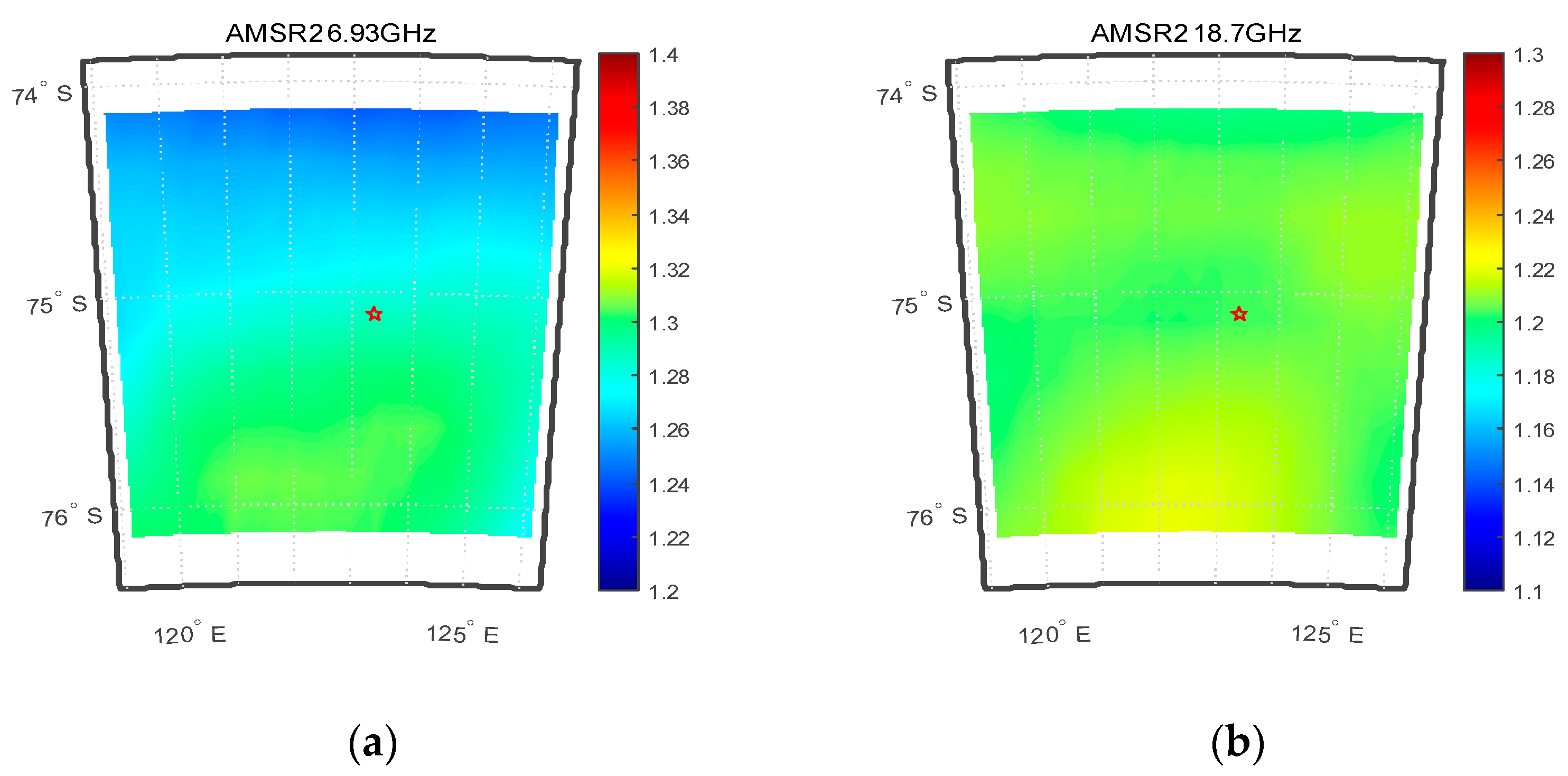
Figure 9 shows the polarization ratio near Dome C station (74.125°S~76.125°S; 119.125°E~126.125°E; about 222 km × 201 km). The value of P in this area is almost stable, indicating that the distribution of snow grain size and snow density in this area is relatively uniform. The snow temperature profile of the whole area can be obtained by using the snow grain size and snow density observed at the Dome-C station. As in
Section 4.1, the area around the Dome-C station with the relatively uniform spatial distribution of snow grain size and snow density has been selected.
6. Conclusions
Microwave BT contains information on snow temperature at different depths, while infrared BT reflects the temperature of the snow surface. Thus, snow temperature profiles can be retrieved by combining multi-frequency microwave BT with infrared BT. In addition, different weight functions are necessary for microwave BT at different frequencies because of the different penetration depths of different frequencies. A conjoint inversion algorithm for inverting snow temperature profiles is developed by combining weighted multi-frequency microwave BT with synthesis infrared BT. The synthesis infrared BT is the integral of infrared BT weighted by microwave antenna pattern, while the weight functions are applied to the microwave BT, and the atmospheric correction is also taken into consideration.
The snow temperature profile data are retrieved based on AMSR2 microwave BT data and MODIS infrared BT data in 2017 and 2018, which are evaluated by comparing with the measured snow temperature data at the Dome-C station. The change of the conjoint inverted snow temperature is consistent with the observation data from the Dome-C station over time at different depths. The mean bias and standard deviation of the conjoint inverted snow temperature are smaller at the deeper layer than that of the snow surface, and the relative accuracy of the conjoint inverted snow temperature is worse at the deeper level than that of the snow surface. Multi-frequency microwave brightness temperature can be used to invert the snow temperature profiles; however, the inverted snow surface temperature is more accurate by combining the infrared BT with the microwave BT in the conjoint inversion algorithm.
Author Contributions
Conceptualization, Z.C. and Q.L.; methodology and validation, Z.C.; theory analysis, R.J., K.C., L.Z. and Z.C.; investigation, L.Z.; writing—preparation, discussion and editing, Z.C., Q.L., R.J. and K.C.; funding acquisition, Q.L. All authors have read and agreed to the published version of the manuscript.
Funding
This work was supported by the National Natural Science Foundation of China (42276183, 42275141).
Conflicts of Interest
The authors declare no conflict of interest.
References
- Rignot, E.; Velicogna, I.; van den Broeke, M.R.; Monaghan, A.; Lenaerts, J.T.M. Acceleration of the contribution of the Greenland and Antarctic ice sheets to sea level rise. Geophys. Res. Lett. 2011, 38, 5. [Google Scholar] [CrossRef] [Green Version]
- Van Liefferinge, B.; Pattyn, F. Using ice-flow models to evaluate potential sites of million year-old ice in Antarctica. Clim. Past 2013, 9, 2335–2345. [Google Scholar] [CrossRef] [Green Version]
- Weller, G.; Schwerdtfeger, P. Thermal properties and heat transfer processes of low-temperature snow. Antarct. Res. Ser. 1977, 25, 27–34. [Google Scholar]
- Durand, G.; Weiss, J. EPICA Dome C Ice Cores Grain Radius Data; IGBP P AGES/World Data Center for Paleoclimatology Data Contribution Series #2004-039; NOAA/NGDC Paleoclimatology Program: Boulder, CO, USA, 2004. [Google Scholar]
- Baker, I.; Obbard, R. Microstructural Location and Composition of Impurities in Polar Ice Cores; US Antarctic Program (USAP) Data Center: Boulder, CO, USA, 2010. [Google Scholar]
- Freville, H.; Brun, E.; Picard, G.; Tatarinova, N.; Arnaud, L.; Lanconelli, C.; Reijmer, C.; Van den Broeke, M. Using MODIS land surface temperatures and the Crocus snow model to understand the warm bias of ERA-Interim reanalyses at the surface in Antarctica. Cryosphere 2014, 8, 1361–1373. [Google Scholar] [CrossRef] [Green Version]
- Brogioni, M.; Macelloni, G.; Pettinato, S. Estimation of air and surface temperature evolution of the East Antarctic Sheet by means of passive microwave remote sensing. In Proceedings of the 2011 IEEE Geoscience and Remote Sensing Symposium (IGARSS), Vancouver, BC, Canada, 24–29 July 2011; pp. 3859–3862. [Google Scholar]
- Maeda, T.; Taniguchi, Y.; Imaoka, K. GCOM-W1 AMSR2 Level 1R Product: Dataset of Brightness Temperature Modified Using the Antenna Pattern Matching Technique. IEEE Tran. Geosci. Remote Sens. 2016, 54, 770–782. [Google Scholar] [CrossRef]
- King, M.D.; Kaufman, Y.J.; Menzel, W.P.; Tanre, D. Remote sensing of cloud, aerosol, and water vapor properties from the moderate resolution imaging spectrometer (MODIS). IEEE Tran. Geosci. Remote Sens. 1992, 30, 2–27. [Google Scholar] [CrossRef] [Green Version]
- Walton, C.C.; Pichel, W.G.; Sapper, J.F.; May, D.A. The development and operational application of nonlinear algorithms for the measurement of sea surface temperatures with the NOAA polar-orbiting environmental satellites. J. Geophys. Res. Oceans 1998, 103, 27999–28012. [Google Scholar] [CrossRef]
- Chen, Z.; Jin, R.; Li, Q.; Zhao, G.; Xiao, C.; Lei, Z.; Huang, Y. Joint Inversion Algorithm of Sea Surface Temperature from Microwave and Infrared Brightness Temperature. IEEE Tran. Geosci. Remote Sens. 2022, 60, 4207013. [Google Scholar] [CrossRef]
- McMillin, L.M.; Crosby, D.S. Theory and validation of the multiple window sea surface temperature technique. J. Geophys. Res. Oceans 1984, 89, 3655–3661. [Google Scholar] [CrossRef]
- Ulaby, F.; Long, D. Microwave Radar and Radiometric Remote Sensing; University of Michigan Press: Ann Arbor, MI, USA, 2014. [Google Scholar]
- Wentz, F.J.; Meissner, T. Algorithm Theoretical Basis Document: AMSR Ocean Algorithm; Remote Sensing Systems: Santa Rosa, CA, USA, 2000. [Google Scholar]
- Surdyk, S. Using microwave brightness temperature to detect short-term surface air temperature changes in Antarctica: An analytical approach. Remote Sens. Environ. 2002, 80, 256–271. [Google Scholar] [CrossRef]
- Jay Zwally, H. Microwave Emissivity and Accumulation Rate of Polar Firn. J. Glaciol. 1977, 18, 195–215. [Google Scholar] [CrossRef] [Green Version]
- Hall, D.K.; Key, J.R.; Case, K.A.; Riggs, G.A.; Cavalieri, D.J. Sea ice surface temperature product from MODIS. IEEE Tran. Geosci. Remote Sens. 2004, 42, 1076–1087. [Google Scholar] [CrossRef]
- Wiesmann, A.; Mätzler, C. Microwave Emission Model of Layered Snowpacks. Remote Sens. Environ. 1999, 70, 307–316. [Google Scholar] [CrossRef]
- Pulliainen, J.T.; Grandell, J.; Hallikainen, M.T. HUT snow emission model and its applicability to snow water equivalent retrieval. IEEE Tran. Geosci. Remote Sens. 1999, 37, 1378–1390. [Google Scholar] [CrossRef]
- Picard, G.; Brucker, L.; Roy, A.; Dupont, F.; Fily, M.; Royer, A.; Harlow, C. Simulation of the microwave emission of multi-layered snowpacks using the dense media radiative transfer theory: The DMRT-ML model. Geosci. Model Dev. 2013, 6, 1061–1078. [Google Scholar] [CrossRef] [Green Version]
- Mätzler, C.; Wiesmann, A. Extension of the Microwave Emission Model of Layered Snowpacks to Coarse-Grained Snow. Remote Sens. Environ. 1999, 70, 317–325. [Google Scholar] [CrossRef]
- Pan, J.; Durand, M.; Sandells, M.; Lemmetyinen, J.; Kim, E.J.; Pulliainen, J.; Kontu, A.; Derksen, C. Differences Between the HUT Snow Emission Model and MEMLS and Their Effects on Brightness Temperature Simulation. IEEE Tran. Geosci. Remote Sens. 2016, 54, 2001–2019. [Google Scholar] [CrossRef]
- Weise, T.; Matzler, C. Radiometric and structural measurements of snow samples. In Proceedings of the 1995 IEEE Geoscience and Remote Sensing Symposium (IGARSS), Firenze, Italy, 10–14 July 1995; pp. 1762–1764. [Google Scholar]
- Macelloni, G.; Brogioni, M.; Pampaloni, P.; Cagnati, A. Multifrequency Microwave Emission Fromthe Dome-C Area on the East Antarctic Plateau: Temporal and Spatial Variability. IEEE Tran. Geosci. Remote Sens. 2007, 45, 2029–2039. [Google Scholar] [CrossRef]
- Bingham, A.W.; Drinkwater, M.R. Recent changes in the microwave scattering properties of the Antarctic ice sheet. IEEE Trans. Geosci. Remote Sens. 2000, 38, 1810–1820. [Google Scholar] [CrossRef]
- Picard, G.; Brucker, L.; Fily, M.; Gallée, H.; Krinner, G. Modeling time series of microwave brightness temperature in Antarctica. J. Glaciol. 2009, 55, 537–551. [Google Scholar] [CrossRef] [Green Version]
- Rott, H.; Sturm, K.; Miller, H. Active and passive microwave signatures of Antarctic firn by means of field measurements and satellite data. Ann. Glaciol. 1993, 17, 337–343. [Google Scholar] [CrossRef] [Green Version]
- West, R.D.; Winebrenner, D.P.; Tsang, L.; Rott, H. Microwave emission from density-stratified Antarctic firn at 6 cm wavelength. J. Glaciol. 1996, 42, 63–76. [Google Scholar] [CrossRef] [Green Version]
| Disclaimer/Publisher’s Note: The statements, opinions and data contained in all publications are solely those of the individual author(s) and contributor(s) and not of MDPI and/or the editor(s). MDPI and/or the editor(s) disclaim responsibility for any injury to people or property resulting from any ideas, methods, instructions or products referred to in the content. |
© 2023 by the authors. Licensee MDPI, Basel, Switzerland. This article is an open access article distributed under the terms and conditions of the Creative Commons Attribution (CC BY) license (https://creativecommons.org/licenses/by/4.0/).


