Airspace Contamination by Volcanic Ash from Sequences of Etna Paroxysms: Coupling the WRF-Chem Dispersion Model with Near-Source L-Band Radar Observations

Abstract

Volcanic emissions (ash, gas, aerosols) dispersed in the atmosphere during explosive eruptions generate hazards affecting aviation, human health, air quality, and the environment. We document for the first time the contamination of airspace by very fine volcanic ash due to sequences of transient ash plumes from Mount Etna. The atmospheric dispersal of sub-10 μm (PM10) ash is modelled using the WRF-Chem model, coupled online with meteorology and aerosols and offline with mass eruption rates (MERs) derived from near-vent Doppler radar measurements and inferred plume altitudes. We analyze two sequences of paroxysms with widely varied volcanological conditions and contrasted meteorological synoptic patterns in October–December 2013 and on 3–5 December 2015. We analyze the PM10 ash dispersal simulation maps in terms of time-averaged columnar ash density, concentration at specified flight levels averaged over the entire sequence interval, and daily average concentration during selected paroxysm days at these flight levels. The very fine ash from such eruption sequences is shown to easily contaminate the airspace around the volcano within a radius of about 1000 km in a matter of a few days. Synoptic patterns with relatively weak tropospheric currents lead to the accumulation of PM10 ash at a regional scale all around Etna. In this context, closely interspersed paroxysms tend to accumulate very fine ash more diffusively at a lower troposphere and in stretched ash clouds higher up in the troposphere. Low-pressure, high-winds weather systems tend to stretch ash clouds into ~100 km wide clouds, forming large-scale vortices 800–1600 km in diameter. Daily average PM10 ash concentrations commonly exceed the aviation hazard threshold, up to 1000 km downwind from the volcano and up to the upper troposphere for intense paroxysms. Vertical distributions show ash cloud thicknesses in the range 0.7–3 km, and PM10 sometimes stagnates at ground level, which represent a potential health hazard.

1. Introduction

1.1. Volcanic Ash Hazards in Aviation

During explosive eruptions, large quantities of volcanic material (gas, ash, aerosols) are injected into the atmosphere as an ash plume, reaching tropospheric and sometimes even stratospheric heights. The subsequent ash cloud drifts, according to the dominant winds in altitude, generate hazards for aviation, human health, and the environment (pollution), both in the short and long term. Whereas lapilli and coarse ash (>1 mm in diameter) fall out within an hour, fine ash (<1 mm, atmospheric residence > 30 min) and especially very fine ash (<30 μm, atmospheric residence from three hours to several days) are agents for volcanic cloud hazards to aircraft and aviation services [1]. The impacts can include engine power loss, blockage of sensors, impaired vision owing to windscreen damage, contamination of aircraft ventilation and pressurization systems, health risks to crew and passengers, abrasive damage to the aircraft exterior, malfunction of the electric/electronic elements with potential short-circuits, maneuvers for cloud avoidance, flight disruptions, deposits of volcanic ash on runways, limited ground operations, airspace and airport closure, and all the subsequent implications for travelling passengers [2]. Because very fine ash is often dispersed thousands of kilometers from the source volcano, it may remain for weeks in the atmosphere in amounts hardly detectable by aircraft, air traffic control, and weather radars, or even visually. Ash products from satellite imagery used for real-time monitoring (e.g., Jiménez-Escalona et al. [3]) sometimes also fail to detect ash due to: (1) overcast weather, (2) mask effects from very fine ash acting as cloud condensation and ice nuclei resulting in a mixed plume/cloud containing liquid water, SO₂, and ice, as reported by Marchese et al. [4] for the 3 December 2015 paroxysm at Etna, and (3) dilute particle concentrations below the detection threshold in distal areas. Even when ash is detected, communication delays to aircraft after the hazard occurrence time remain another limitation. In our study, we model the dispersion of ash particles considering ten bins of volcanic ash with diameters ranging from 2 mm down to less than 3.9 μm. Specific interest is devoted to ash particles less than 10 μm in size (PM10), as these are also well-known to affect air quality and human health (sub-10 μm inhalable volcanic ash, including the subset of respirable volcanic ash below 4 μm) (e.g., Eychenne et al. [5]). Very fine volcanic ash, SO₂, and aerosols further impact the environment and climate through radiative forcing (e.g., Sellito et al. [6]).

The modelling of volcanic plume transport has attracted increasing attention from the natural hazard research community because of the impact of volcanic emissions dispersal on aviation and the economy. The global economic impact of the eruption of Eyjafjallajökull in 2010 was estimated by Oxford Economics to be ~USD 5 billion, with about USD 2 billion in direct financial losses to the aviation industry. According to EUROCONTROL [7], it could be more than halved owing to improvements achieved in the last decade in the air sector regarding crisis management and optimized operational performance. For example, cost-based trajectory optimization based on dispersion models and flight planning software decreases the cost and disruption to air traffic deriving from volcanic events [8].

The number of reported aircraft encounters with volcanic ash clouds causing various degrees of airframe or engine damage amounted to 129 between 1953 and 2009 [9], and to 113 between 2010 and 2014 [10]; however, not all encounters are reported and, therefore, the number remains underestimated. While the most damaging encounters have occurred within 24 h of eruption onset and/or within 1000 km of the source, less safety-significant, but still economically damaging, encounters have occurred at greater distances and extended times [9]. In parallel, the total number of passengers transported each year also increases, including by a factor of 2.8 in the two decades preceding 2019 when it reached over 4.5 billion people [2].

As demonstrated in this paper, Mount Etna emissions present significant hazards to regional air traffic, in addition to significant economic losses. The closest international aeronautic infrastructure, Catania airport, must frequently limit its services because of Etna ash emissions, leading to numerous rerouted or cancelled flights and airport closures. About 11 million commercial passengers transited through Catania airport in 2022 (6.4 and 7.1 million in 2013 and 2015, respectively), utilizing about 76,000 flights in 2022 involving 86 routes to domestic and European destinations (https://cataniaairport.com/statistics/; accessed on 3 May 2023).

1.2. Volcanic Ash Advisories on Etna

With the purpose of keeping aviators informed about volcanic hazards, the International Civil Aviation Organization (ICAO) established nine Volcanic Ash Advisory Centres (VAACs) covering the world as part of the International Airways Volcano Watch (IAVW). Each of the nine centers under the IAVW respond to reports of volcanic ash within their region and provide the aviation community with information on the ash cloud’s current location and forecasts on the future extent in the case of significant volcanic eruptions. Ash warnings issued by the VAACs are in the form of standardized Volcanic Ash Advisory messages (VAA, sometimes including Graphics: VAG) based on a Volcano Observatory Notice for Aviation (VONA), aircraft in flight (AIREP) and governmental agencies utilizing meteorological ground stations and satellite imagery (SIGMET, NOTAM, ASHTAM) (https://www.ssd.noaa.gov/VAAC/vaac.html, accessed on 10 February 2023).

The Toulouse VAAC operated by Météo-France (https://vaac.meteo.fr/, accessed on 10 February 2023), with the London VAAC as a backup, is in charge of the nowcasting of volcanic emissions dispersal in a very large zone of the globe, including the Mediterranean basin, which hosts very active volcanoes like Etna and Stromboli. Between 2006 and 2022, the Toulouse VAAC released 792 Volcanic Ash Advisories (VAA, most including Graphics: VAG) for Etna, including 22 and 29 during/following the eruptions from the two sequences analyzed in this paper (Table 1, Table 2 and

Table A1. VAA issued by the Toulouse VAAC, Météo-France, for the 2013 and 2015 eruptive sequences. NIL = no ash cloud is produced; yellow = advisory; orange = watch; red = warning.

N	VA Advisory (UTC)	Aviation Color Code	Eruption Details
1	ETNA—2013-10-26 06:00	NIL	STARTED AT 0200Z
2	ETNA—2013-10-26 06:00	NIL	STARTED AT 0200Z
3	ETNA—2013-10-26 11:30	NIL	STOPPED AROUND 1100Z
4	ETNA—2013-10-26 17:30	NIL	STOPPED AROUND 1100Z
5	ETNA—2013-10-27 08:13	NIL	CLOUD SEEMS TO BE COMPOSED OF WATER VAPOUR, NO SIGNAL OF ASH NEITHER VOLCANIC GAS ON SAT IMAGERY
6	ETNA—2013-10-28 16:00	NIL	VA NOT IDENTIFIABLE
7	ETNA—2013-10-29 10:50	NIL	UNKNOWN
8	ETNA—2013-11-11 03:43	NIL	UNKNOWN
9	ETNA—2013-11-11 10:11	NIL	CLOUD IDENTIFIABLE ON WEBCAM MAY CONTAIN VA
10	ETNA—2013-11-16 23:03	NIL	IN PROGRESS LOW INTENSITY
11	ETNA—2013-11-17 02:17	NIL	GOING ON
12	ETNA—2013-11-17 05:09	NIL	ERUPTION STOPPED ABOUT 0500Z
13	ETNA—2013-11-17 11:29	NIL	ERUPTION ENDED
14	ETNA—2013-11-23 10:07	NIL	ASH CLOUD OF SEVERE INTENSITY STARTS AT 0930Z
15	ETNA—2013-11-23 11:17	NIL	ERUPTION ENDED AT 1030Z
16	ETNA—2013-11-23 14:26	NIL	ERUPTION ENDED AT 1030Z
17	ETNA—2013-11-23 20:19	NIL	ERUPTION ENDED
18	ETNA—2013-11-28 17:37	NIL	ERUPTION HAS STARTED AT 1730Z, GOING ON
19	ETNA—2013-11-28 19:50	NIL	ERUPTION HAS RESTARTED AT 1930Z, GOING ON
20	ETNA—2013-11-28 23:45	NIL	ERUPTION HAS STOPPED AT 2330Z
21	ETNA—2013-12-02 19:00	NIL	ERUPTION HAS STARTED AT 1820Z, GOING ON
22	ETNA—2013-12-02 23:40	NIL	ERUPTION ENDED AT 2300Z
1	ETNA—2015-12-02 23:00	ORANGE	STROMBOLIAN ACTIVITY
2	ETNA—2015-12-03 02:41	RED	EXPLOSIVE ERUPTION OCCURRED AT 02000Z
3	ETNA—2015-12-03 04:00	ORANGE	ERUPTION AND ASH EMISSION DECREASING. VA IDENTIFIABLE FM SATELLITE IMAGERY
4	ETNA—2015-12-03 10:00	ORANGE	SMALL ACTIVITY IN VICINITY OF VOLCANO
5	ETNA—2015-12-03 14:00	YELLOW	NO SIGNIFICANT ASH EMISSION
6	ETNA—2015-12-04 09:40	RED	ASH EMISSION VISIBLE ON WEBCAM
7	ETNA—2015-12-04 10:45	RED	ERUPTION ONGOING
8	ETNA—2015-12-04 15:45	RED	ASH PLUME NEAR SUMMIT VOLCANO
9	ETNA—2015-12-04 21:00	RED	ERUPTION STARTED AT 2045Z
10	ETNA—2015-12-05 03:00	RED	STROMBOLIAN EXPLOSIONS
11	ETNA—2015-12-05 08:45	RED	STROMBOLIAN EXPLOSIONS
12	ETNA—2015-12-05 15:00	ORANGE	SOME VOLCANIC ASH NEAR THE SUMMIT
13	ETNA—2015-12-05 15:05	RED	SIGNIFICANT EMISSION OF ASH OVER THE VOLCANO
14	ETNA—2015-12-05 20:31	ORANGE	EXPLOSIVE ACTIVITY AND SIGNIFICANT ASH EMISSION STOPPED
15	ETNA—2015-12-06 11:45	ORANGE	VOLCANIC ASH NEAR THE SUMMIT
16	ETNA—2015-12-06 12:00	ORANGE	VOLCANIC ASH NEAR THE SUMMIT
17	ETNA—2015-12-06 13:00	RED	INCREASING ACTIVITY
18	ETNA—2015-12-06 17:55	RED	ONGOING MODERATE INTENSITY
19	ETNA—2015-12-06 23:00	RED	EXPLOSIVE ACTIVITY
20	ETNA—2015-12-07 03:00	RED	ACTIVITY STILL ONGOING
21	ETNA—2015-12-07 09:00	ORANGE	ACTIVITY STILL ONGOING
22	ETNA—2015-12-07 15:00	RED	VA NOT IDENTIFIABLE FM SAT DATA, WINDS FL100 280/10KT FL300 290/15KT
23	ETNA—2015-12-07 20:50	RED	SPORADIC ERUPTIONS STILL GOING ON
24	ETNA—2015-12-08 03:00	RED	SPORADIC ERUPTIONS STILL GOING ON
25	ETNA—2015-12-08 09:00	ORANGE	STROMBOLIAN ACTIVITY HAS DECREASED
26	ETNA—2015-12-09 04:00	ORANGE	ERUPTION STILL GOING ON
27	ETNA—2015-12-09 09:17	RED	ERUPTION STILL GOING ON
28	ETNA—2015-12-09 14:50	RED	SEEMS TO BE DECREASING
29	ETNA—2015-12-09 20:45	ORANGE	WEAK ERUPTIVE ACTIVITY IS ONGOING

). The reaction time of the VAACs depends mainly on the on-site volcano observatory that must provide a VONA with critical information about the ongoing activity and input parameters in a timely manner. At Etna, the all-year 24/7 monitoring is mainly carried out by the INGV Osservatorio Etneo, transmitting VONA, but also by information provided to the Italian Department of Civil Protection (https://www.protezionecivile.gov.it/en/, accessed on 11 February 2023) through specific communication procedures during crises.

As for volcanic hazards to aviation, present challenges include the detection of volcanic ash clouds, the accurate forecasting of their dispersion, and the timely and targeted communication of this information. Dispersion model simulations may contribute to the evaluation of the space–time distribution of volcanic constituents (solid particles, gases, aerosols), including for ash dispersal nowcasting as implemented by the VAACs during eruptions. Understanding engine and airframe tolerances to ash ingestion and gas effects would further inform the operational risk management of airlines.

1.3. Improving Ash Dispersal Modelling: Coupling WRF-Chem and Time-Varying Eruption Source Parameters

Despite the knowledge gained from remote sensing data and the numerical modelling of volcanic eruptions, the identification of hazard areas around active volcanoes still remains a considerable scientific challenge [11]. The parameters that most influence the forecast of ash column loading distributions for mapping flight hazard areas are the free troposphere turbulence levels, the precipitation threshold for wet deposition, and eruption source parameters, such as plume height and the mass eruption rate (MER), and the onset and end times of the paroxysm [12,13,14]. Egan et al. [15] have implemented a simplified volcanic ash aggregation scheme into the Weather Research Forecasting model with Chemistry (WRF-Chem; Grell et al. [16]), for computing the aggregation rate coupled with the atmospheric environment at each model step. Harvey et al. [13] listed the observation of plume height through mobile radars among the top research priorities for reducing uncertainties in forecasts on the long-range transport of volcanic ash. The WRF-Chem model has recently been utilized [17] to model the volcanic plumes associated with Etna’s paroxysmal episodes on 3–7 December 2015 that led to the closure of the nearby Catania International Airport. It emerged that the WRF-Chem model reasonably reproduced the distribution of SO₂ and volcanic ash, as compared with multi-platform data from satellite sensors and Doppler radars. More recently, Rizza et al. [18] have demonstrated the need for time-dependent eruption source parameters (ESP), together with the correct specification for the injection height to properly describe the transport of Etna volcanic ash in the Mediterranean basin. The online coupling between chemistry/aerosols with meteorology represents an innovative development in the current volcanic ash transport and dispersion models (VATDM), as it avoids any space–time interpolation by considering the two-way feedback for all the processes (meteorology, chemistry, and physics) at the time step level, in the context of time-varying ESP [18].

The main aim of this paper is to document the large-scale contamination of airspace by a succession of closely interspersed explosive eruptions, providing insight on the hazards to air traffic and the atmospheric dispersion of volcanic pollutants. It also demonstrates the usefulness and good potential of nowcasting of ground-based near-vent radar observations to provide the most realistic source term estimates for volcanic ash that will undergo long-range transportation. For these purposes, we use MER retrievals from an L-band Doppler radar (carrier frequency 1.274 GHz) monitoring Etna (VOLDORAD-2B, here noted as V2B; [19,20]) as input into the WRF-Chem atmospheric model simulations, to evaluate the regional-scale dispersion and accumulation of very fine volcanic ash released by successive paroxysms. This full coupling methodology, using measured time-evolving source parameters, accurately reproduces the atmospheric dispersal from volcanic transient emissions, as attested by satellite imagery from various gas and ash sensors during the 23 November 2013 paroxysm [18]. The higher time resolution in the definition on the meteorological conditions and the specification of the eruption conditions allows for the reduction in the related uncertainties present in the modelling of the transportation and dispersal of tephra in the atmosphere.

In the present study, we analyze two test case eruptive sequences at Etna, the first one including six successive paroxysms from the New Southeast crater (NSE) that occurred in 38 days between October 26 and 2 December 2013, the second sequence including four paroxysms from the Voragine crater (VOR) that occurred in less than 3 days between 3 and 5 December 2015. The methods and data used in this study are described in Section 2, which also describes the details of the two eruptive sequences, the volcanic emission estimates determined using the V2B radar data, and the model setup. In Section 3, we discuss the modelling results, in terms of the meteorological and ash transportation characteristics in the numerical model domain. The conclusions and aims for future works are presented in Section 4.

2. Materials and Methods

2.1. Description of the Two Eruptive Sequences

2.1.1. The 2013 Sequence: 26 October to 2 December

The first simulation reproduces the sequence of paroxysms that occurred at the New Southeast (NSE) crater from 26 October to 2 December 2013 (Table 1, Figure 1). After a 6 month quiescence, a new paroxysm began on 26 October at the NSE crater. For this event, the SO₂ mass detected by the OMI (Ozone Monitoring Instrument) sensor onboard the Aura satellite peaked at 0.77 kilotons (https://so2.gsfc.nasa.gov/index.html, accessed on 5 May 2023). The October–December sequence includes six paroxysms featuring the usual lava fountain feeding many kilometers high tephra plumes, ranging in duration from 3.2 to 10 h and from 2.9 × 10⁴ to 3.9 × 10⁵ kg s⁻¹ for the average MER (peaks: 2.1 × 10⁵ to 8.9 × 10⁶ kg s⁻¹), as retrieved from the VOLDORAD-2B radar (Table 1). Only the last three paroxysms punctually exceeded 10⁶ kg s⁻¹, the shortest and most violent in the series occurred during strong westerly wind on November 23 [18,21,22]. This paroxysm averaged nearly 4 × 10⁵ kg s⁻¹ during 193 min, including 3.5 × 10⁶ kg s⁻¹ sustained during its 16 min climax phase, which released 80% of the total erupted mass of pyroclasts at maximum velocities over 200 m s⁻¹ [20]. The six successive paroxysms released in total about 18.9 × 10⁹ kg of tephra, with respective mass contributions of 18, 40, 24, 5, 8, and 5%.

Plume top altitudes for this sequence (8.1–11.1 km a.s.l.) can be found in the work of Corradini et al. [23]. The Toulouse VAAC, Météo-France, released 23 VAAs for Etna during the period of the six paroxysms for flight levels up to FL380 (11.58 km a.s.l.) with wind speed estimates up to 35 m s⁻¹.

Table 1. Onset/end of each paroxysm in the 2013 sequence and the mass eruption rates (MERs) obtained by the VOLDORAD-2B radar system. Volcanic Explosivity Index (VEI) from the MSVOLSO2L4 database (nd = no data or undetermined). Number of Volcanic Ash Advisories (VAAs) released from the Toulouse VAAC, Météo-France (https://vaac.meteo.fr/, accessed on 16 May 2023).

	2013	Julian Day	Start (UTC)	End (UTC)	Duration	Bins	V2B MER (kg s−1)	VEI	VAA
Paroxysm	Date	Start	HH:MM	HH:MM	HH:MM	Range in m (Bin Number)	Average (Max)
NSE1	26 October	299	01:35	10:27	08:52	3135–3285 (3; 4)	2.9 × 104 (2.1 × 105)	2	7
NSE2	11 November	315	00:01	11:52	11:51	3135–3285 (3; 4)	3.6 × 104 (2.3 × 105)	2	2
NSE3	16–17 November	320–321	22:14 (16/11)	04:35 (17/11)	05:21	3135–3285 (3; 4)	4.3 × 104 (2.8 × 105)	nd	4
NSE4	23 November	327	07:13	10:26	03:13	3135–3285 (3; 4)	3.9 × 105 (8.9 × 106)	2	4
NSE5	28 November	332	15:15	23:35	08:20	3135–3285 (3; 4)	2.5 × 105 (1.3 × 106)	nd	3
NSE6	2 December	336	19:08	22:42	03:34	3135–3285 (3; 4)	2.5 × 105 (1.8 × 106)	2	2

Table 1. Onset/end of each paroxysm in the 2013 sequence and the mass eruption rates (MERs) obtained by the VOLDORAD-2B radar system. Volcanic Explosivity Index (VEI) from the MSVOLSO2L4 database (nd = no data or undetermined). Number of Volcanic Ash Advisories (VAAs) released from the Toulouse VAAC, Météo-France (https://vaac.meteo.fr/, accessed on 16 May 2023).

	2013	Julian Day	Start (UTC)	End (UTC)	Duration	Bins	V2B MER (kg s−1)	VEI	VAA
Paroxysm	Date	Start	HH:MM	HH:MM	HH:MM	Range in m (Bin Number)	Average (Max)
NSE1	26 October	299	01:35	10:27	08:52	3135–3285 (3; 4)	2.9 × 104 (2.1 × 105)	2	7
NSE2	11 November	315	00:01	11:52	11:51	3135–3285 (3; 4)	3.6 × 104 (2.3 × 105)	2	2
NSE3	16–17 November	320–321	22:14 (16/11)	04:35 (17/11)	05:21	3135–3285 (3; 4)	4.3 × 104 (2.8 × 105)	nd	4
NSE4	23 November	327	07:13	10:26	03:13	3135–3285 (3; 4)	3.9 × 105 (8.9 × 106)	2	4
NSE5	28 November	332	15:15	23:35	08:20	3135–3285 (3; 4)	2.5 × 105 (1.3 × 106)	nd	3
NSE6	2 December	336	19:08	22:42	03:34	3135–3285 (3; 4)	2.5 × 105 (1.8 × 106)	2	2

2.1.2. The 2015 Sequence: 3–5 December

An exceptionally rapid sequence of eruptive episodes occurred in December 2015, generating powerful eruption columns during the paroxysms, tall lava fountains, Strombolian activity, lava flow emissions, and persistent ash emissions, involving all four summit craters at different times [24,25]. This activity culminated with four paroxysmal events on 3–5 December 2015 from the Voragine (VOR) crater, constituting the second sequence in our analysis (Table 2, Figure 2). As with most paroxysms at Etna, they were preceded by Strombolian activity and displayed lava fountains and, subsequent, high tephra plumes. These paroxysms were short (less than 1.5 h) and not accompanied by lava flows and, compared with the 2013 sequence, they were characterized by exceptional eruptive power and a rapid occurrence rate. They rank among the most violent eruptions in the last two decades, in part due to the depth of the magma source region at 1.5 km b.s.l. [26,27].

Table 2. Onset/end of each paroxysm in the 2015 sequence and the mass eruption rates (MERs) obtained by the V2B radar system. Volcanic Explosivity Index (VEI) from the MSVOLSO2L4 database (nd = no data or undetermined). Number of Volcanic Ash Advisories (VAAs) released from the Toulouse VAAC, Météo-France (https://vaac.meteo.fr/, accessed on 16 May 2023), totaling 29 for 3–9 December.

	2015	Julian Day	Start (UTC)	End (UTC)	Duration	Bins	V2B MER (kg s−1)	VEI	VAA
Paroxysm	Date	Start	HH:MM	HH:MM	HH:MM	Range in m (Bin Number)	Aver (Max)
VOR1	3 December	336	02:00	03:31	01:31	3885–4185 (8; 9; 10)	1.7 × 106 (4.5 × 106)	2	5
VOR2	4 December	337	09:03	10:14	01:11	3735–4035 (7; 8; 9)	1.7 × 105 (5.0 × 105)	nd	3
VOR3	4 December	337	20:26	21:15	00:49	3735–4035 (7; 8; 9)	1.8 × 105 (1.2 × 106)	nd	2
VOR4	5 December	338	14:45	16:10	01:25	3735–4035 (7; 8; 9)	1.0 × 105 (4.1 × 105)	nd	4

Table 2. Onset/end of each paroxysm in the 2015 sequence and the mass eruption rates (MERs) obtained by the V2B radar system. Volcanic Explosivity Index (VEI) from the MSVOLSO2L4 database (nd = no data or undetermined). Number of Volcanic Ash Advisories (VAAs) released from the Toulouse VAAC, Météo-France (https://vaac.meteo.fr/, accessed on 16 May 2023), totaling 29 for 3–9 December.

	2015	Julian Day	Start (UTC)	End (UTC)	Duration	Bins	V2B MER (kg s−1)	VEI	VAA
Paroxysm	Date	Start	HH:MM	HH:MM	HH:MM	Range in m (Bin Number)	Aver (Max)
VOR1	3 December	336	02:00	03:31	01:31	3885–4185 (8; 9; 10)	1.7 × 106 (4.5 × 106)	2	5
VOR2	4 December	337	09:03	10:14	01:11	3735–4035 (7; 8; 9)	1.7 × 105 (5.0 × 105)	nd	3
VOR3	4 December	337	20:26	21:15	00:49	3735–4035 (7; 8; 9)	1.8 × 105 (1.2 × 106)	nd	2
VOR4	5 December	338	14:45	16:10	01:25	3735–4035 (7; 8; 9)	1.0 × 105 (4.1 × 105)	nd	4

The first episode on 3 December was the most powerful, with lava fountain velocities inferred from the V2B averaging 200 m s⁻¹ during the climax and peaking at 250–290 m s⁻¹. An ash plume ascent velocity of 5.6 m s⁻¹ (10 km in height above crater level in about 30 min) is inferred from the timing of the V2B near-source power and velocity increase and the plume top altitudes from the MSG-SEVIRI HOTVOLC data and vertical temperature profiles [28], the maximum plume top altitude of 13.5 ± 1.5 km a.s.l. being reached around 03:00 UTC. The following paroxysms gradually decreased in regard to the MERs, the total mass of erupted pyroclasts, and the lava fountain average height [26].

These paroxysms caused the atmospheric dispersion and widespread ash fallout to more than 100 km away, with disruptive consequences to aviation and aeronautical infrastructure and services. In particular, Catania International Airport reported repeated closures of airspace sectors between 3 and 9 December 2015, and at least 57 cancelled flights, 56 diverted flights, and tens of modified flights on 4–5 December. The Toulouse VAAC, Météo-France, released 29 VAAs in 7 days (3–9 December) for flight levels up to FL350 (10,660 m a.s.l.) and wind speeds up to 15 m s⁻¹, while the INGV released 16 VONA in four days (2–5 December) reporting on these paroxysms.

The regional environmental impact of the volcanic emissions from this short series of paroxysms can be apprehended from estimates of the released product amounts. According to Bonaccorso and Calvari [26], the total production of pyroclasts was 10 × 10⁶ m³ DRE (Dense Rock Equivalent, i.e., about 25 × 10⁹ kg), with respective mass contributions of 41, 27, 19, and 13% for the successive events. The V2B estimates point to 11 × 10⁹ kg, with successive mass contributions of 84.1, 6.5, 4.8, and 4.6%. Differences among the estimates can stem from both the numerous hypotheses used by the former to derive magma volumes from the strainmeter and camera measurements, and from the possible underestimation by the V2B of the last three weaker paroxysms due to the marginal position of the Voragine crater with respect to the radar beam. The SO₂ mass detected by the OMI sensor peaked at 20 kilotons in early December (https://so2.gsfc.nasa.gov/index.html, accessed on 16 May 2023).

The definition of the eruption source parameters (ESP), namely the volcano location in the grid domain, the start and end of each single paroxysm (UTC time), the total grain size distribution (TGSD), the MER, and the injection height, were pre-processed as described in the following paragraphs.

2.2. The VOLDORAD-2B (V2B) Doppler Radar System

2.2.1. Description

Between 2009 and 2022, the INGV-OE monitored Etna’s tephra emissions using a volcano Doppler radar provided by the OPGC (VOLDORAD-2B), jointly operated from the Montagnola station about 3 km south of the New SE crater. This L-band (23.5 cm wavelength) pulse radar probed 13 atmospheric volumes, 150 m deep, right above the summit craters using a fixed pointing antenna beam. The echo power and Doppler velocity parameters (level 1 data) in each range bin are computed following the methodology of Dubosclard et al. [29], at intervals of 0.22 s from 3 incoherent integrations of the Doppler spectra (raw data). These near-source measurements on the emitted tephra are unique as they allow maximum ejection velocities at the base of the eruptive column and the MER (level 2 products) to be determined, potentially in real-time [19,20], and at a satisfying level of uncertainty as revealed by comparisons with other sensors [30,31,32]. During the 2011–2015 period, the V2B radar successfully recorded about 50 paroxysms of vigorous lava fountains feeding tephra plumes up to over 13 km high. The level 1 data are available from an open access database by the Observatoire de Physique du Globe de Clermont-Ferrand (http://voldorad.opgc.fr/bddtr.php, accessed on 16 June 2023; [33]), as well as more elaborated (level 2) products upon request, such as the MER, the onset and end of the fountaining phase, and the eruptive crater.

2.2.2. Data Elaboration

We used the methodology by Freret-Lorgeril et al. [20] to compute the MER from the V2B data. It showed that the product of the measured echo power and radial velocities of rising tephra in the beam volumes located immediately above the eruptive crater is proportional to the MER (i.e., a MER proxy) and correlates with the observed plume heights for many paroxysms at Etna. The calibration constant was then found by comparing the radar proxies with the MER derived from a plume ascent model matching the observed plume heights and including wind vertical profiles [34].

In this study, the MER was computed from range bins displaying the maximum power, at 3135 and 3285 m at a slant distance from the radar for the paroxysms originating from the New SE crater during the first sequence (26 October–2 December 2013, Table 1), and from 3 range gates for the second sequence of paroxysms originating from the Voragine crater (Table 2). The V2B MER data were elaborated to be compatible with the WRF-Chem input system; in particular, they were averaged for a 30 s interval to be integrated into the numerical model at each time step. The corresponding time series for the MER are depicted in Figure 1 and Figure 2 for the 2013 and 2015 eruptive sequences, respectively.

Figure 1. Mass eruption rate from the V2B radar system ingested into the WRF-Chem volcanic package for the 2013 sequence: (a) full sequence, (b) NSE2 paroxysm, (c) NSE3 paroxysm, (d) NSE4 paroxysm, (e) NSE5 paroxysm, and (f) NSE6 paroxysm. Julian day 290 corresponds to 17 October 2013. Units for MER are 10⁶ kg s⁻¹.

Figure 1. Mass eruption rate from the V2B radar system ingested into the WRF-Chem volcanic package for the 2013 sequence: (a) full sequence, (b) NSE2 paroxysm, (c) NSE3 paroxysm, (d) NSE4 paroxysm, (e) NSE5 paroxysm, and (f) NSE6 paroxysm. Julian day 290 corresponds to 17 October 2013. Units for MER are 10⁶ kg s⁻¹.

Figure 2. Mass eruption rate from the V2B radar system ingested into the WRF-Chem volcanic package for the 2015 sequence of paroxysms from the Voragine crater: (a) full sequence, (b) VOR1, (c) VOR2 and VOR3, and (d) VOR4. Julian day 335 corresponds to 2 December 2015. Units for MER are 10⁶ kg s⁻¹.

Figure 2. Mass eruption rate from the V2B radar system ingested into the WRF-Chem volcanic package for the 2015 sequence of paroxysms from the Voragine crater: (a) full sequence, (b) VOR1, (c) VOR2 and VOR3, and (d) VOR4. Julian day 335 corresponds to 2 December 2015. Units for MER are 10⁶ kg s⁻¹.

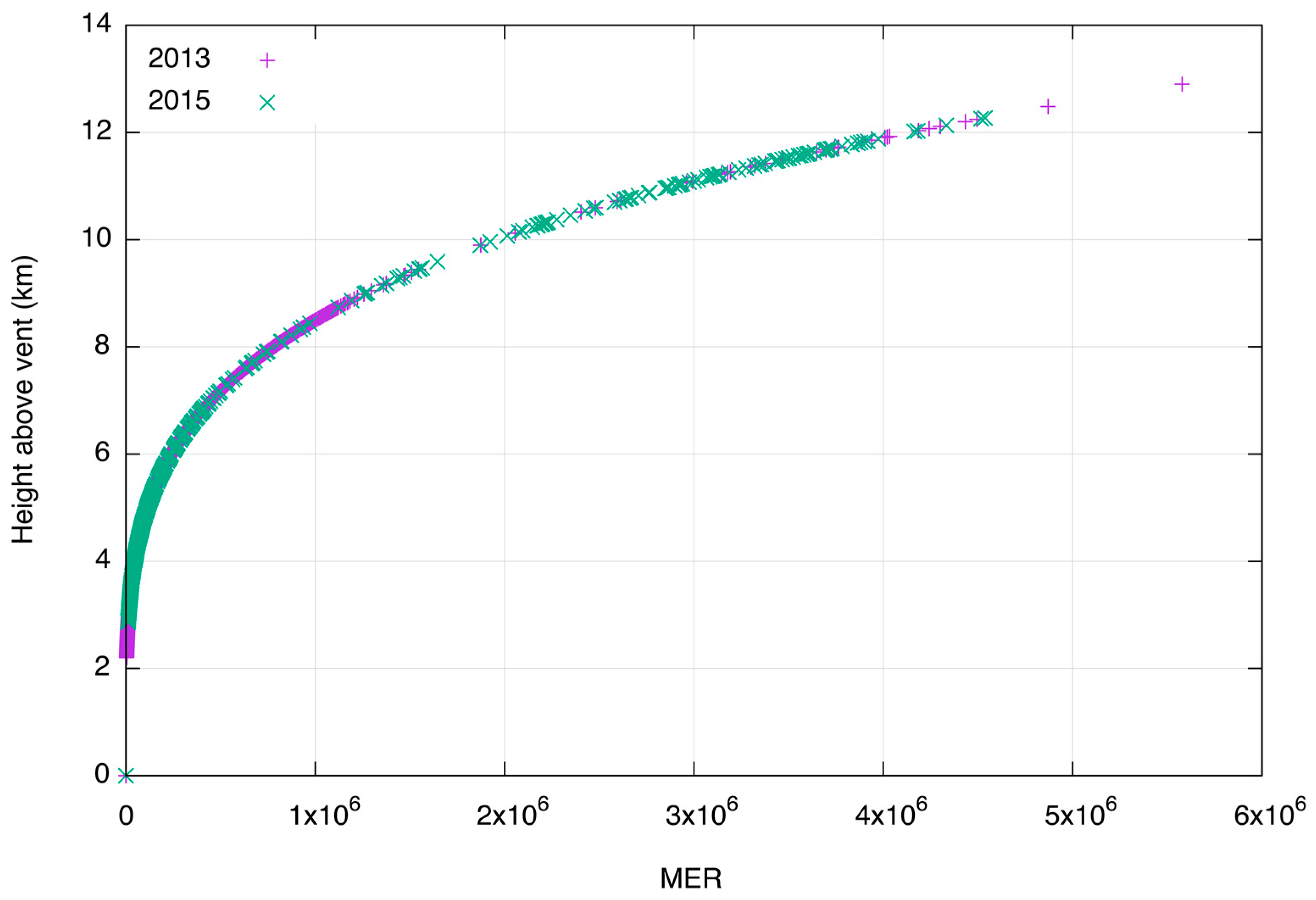
2.3. Determination of the Eruption Height

In case of missing experimental data for the model injection height, the zero-order semi-empirical relationship by Mastin et al. [35] linking column height with the MER observations can be utilized. It is expressed by the following Equation (1) [35], and reported in Figure 3:

$$\mathrm{h}=5\times {10}^{-4}{\left(\frac{\mathrm{M}\mathrm{E}\mathrm{R}}{\mathsf{\rho }}\right)}^{0.241}$$

(1)

where h is expressed in meters (above the vent), ρ denotes the magma density (2600 kg m⁻³), and the MER is obtained by the above-described elaborations of the V2B radar data and reported in Figure 1 and Figure 2.

For the range of mass eruption rates considered in the two series of eruptions [0–6] × 10⁶ kg s⁻¹, the corresponding eruption height has an upper limit of 12–13 km (above the vent), in agreement with Mastin et al. [35] (Figure 1). The MER, derived from the Doppler radar, is highly variable over time and used as input into the WRF-Chem.

The emission profile is specified according to the vertical profile derived from the umbrella cloud model, in which 75% of the erupted mass is constrained in the umbrella cloud and the remaining 25% is linearly distributed from the umbrella base down to the vent [36].

2.4. Model Description and Setup

For this study, the WRF-Chem model version 4.3.1 has been utilized in a numerical domain covering the central Mediterranean region, with 310 × 320 grid points and a horizontal grid spacing of 6 km (1854 × 1914 km²,

Table 3. Physical and chemical options for the WRF-Chem model. In parenthesis, the name-list value.

Microphysics	(7)—4ICE Goddard scheme
LW/SW radiation	(5,5)—New Goddard shortwave and longwave schemes
Surface layer	(2)—Eta similarity scheme
PBL	(2)—Mellor–Yamada–Janjić scheme
Land surface	(4)—Noah-MP land surface model
Initial and boundary conditions	FNL-GFS
chem_opt	(300)—GOCART aerosol model
TGSD	E1 distribution
ESP	MER from V2B radar data Injection heights from Mastin et al. [35]

). The boundary and initial conditions are at 1 degree resolution and are provided from the NCAR/NCEP final analysis from the Global Forecast System (FNL from GFS). The first sequence simulation started at 00:00 UTC on 25 October and ended at 00:00 UTC on 4 December 2013. The second sequence run started at 00:00 UTC on 2 December and ended at 00:00 UTC on 8 December 2015.

The full set of parameterizations for the WRF-Chem model are reported in Table 3.

Based on the WRF setup recommended by Shi et al. [37] and Rizza et al. [38], the following physics schemes are utilized: the Mellor–Yamada–Janjić (MYJ; [39]) and the Eta similarity theory [40] schemes are used to describe the planetary boundary layer (bl_pbl_physics = 2) and the surface layer (sf_sfclay_physics = 2) processes, respectively. The land surface exchange coefficients and the associated fluxes in momentum, heat, and humidity are represented by the Noah-MP land surface model (sf_surface_physics = 4; [41]).

The radiative schemes are parameterized using the Goddard radiation model [42] for the shortwave (ra_sw_physics = 5) and longwave (ra_lw_physics = 5) components. The microphysics parameterization considers the new one-moment Goddard four-class ice (4ICE) scheme developed by Lang et al. [43] and implemented in the early versions (3.4.1) of the WRF package (mp_physics = 7). This scheme has prognostic variables for cloud ice, snow, graupel, and hail.

In the WRF-Chem model, the total grain size distribution (TGSD) consists of ten bins of volcanic ash (vash_#) particles with a grain diameter range starting from 2 mm down to less than 3.9 μm [36] and expressed in mixing ratio units ($\mathsf{\mu }$g kg⁻¹). The corresponding mass fraction percentage is described by the E1 distribution and reported in

Table 4. Total grain size distribution (E1) from Poret et al. [22] and Rizza et al. [18].

Vash_#	1	2	3	4	5	6	7	8	9	10
µm	1000 2000	500 1000	250 500	125 250	62.5 125	31.25 62.5	15.625 31.25	7.8125 15.625	3.90625 7.8125	0 3.90625
wt%	16.7	8.3	10.4	12.5	6.4	12.5	14.6	8.3	6.2	4.2

. It has been recently introduced into the WRF-Chem volcanic package by Rizza et al. [18] and is derived from Poret et al. [22]’s analysis of the experimental data from the 23 November 2013 Etna eruption. The MER, which is used as input into the WRF-Chem model, is derived from the Doppler radar, and it is extremely variable over time.

3. Results and Discussion: Hazard Maps

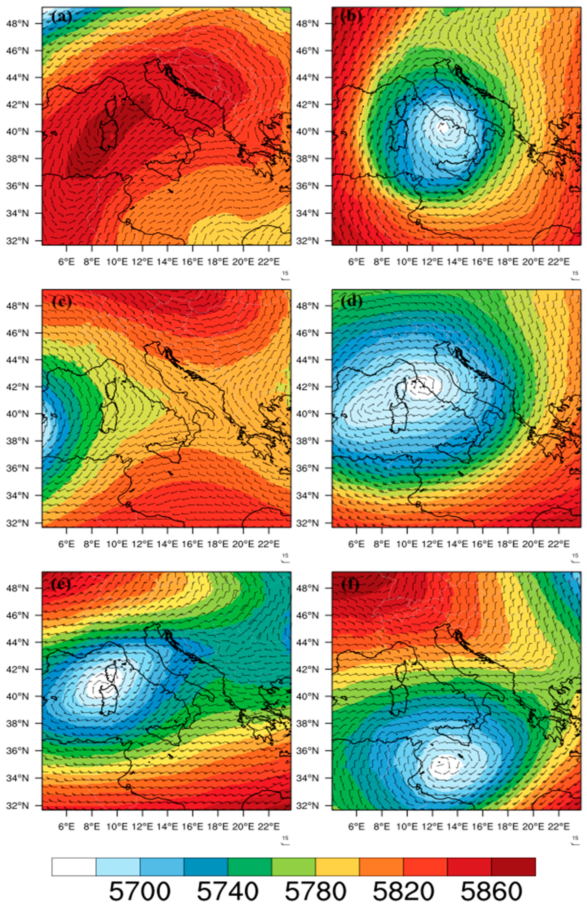
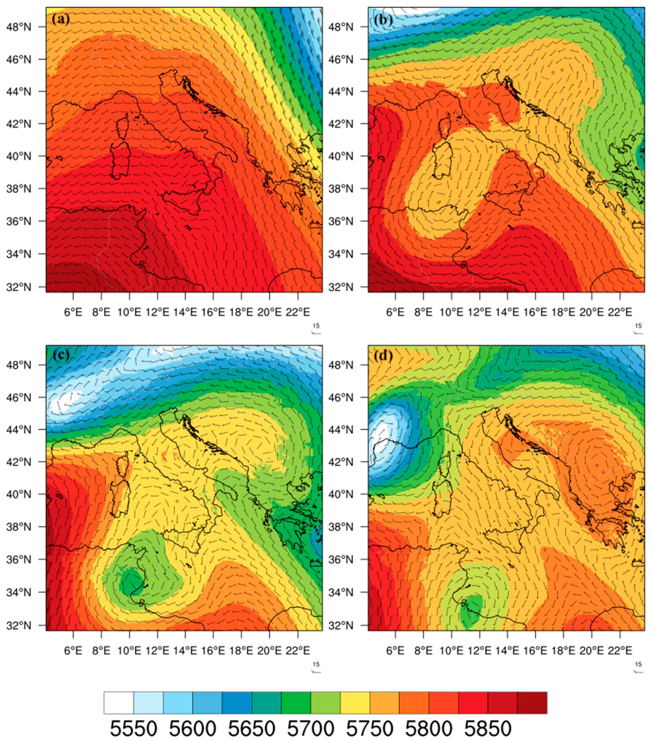
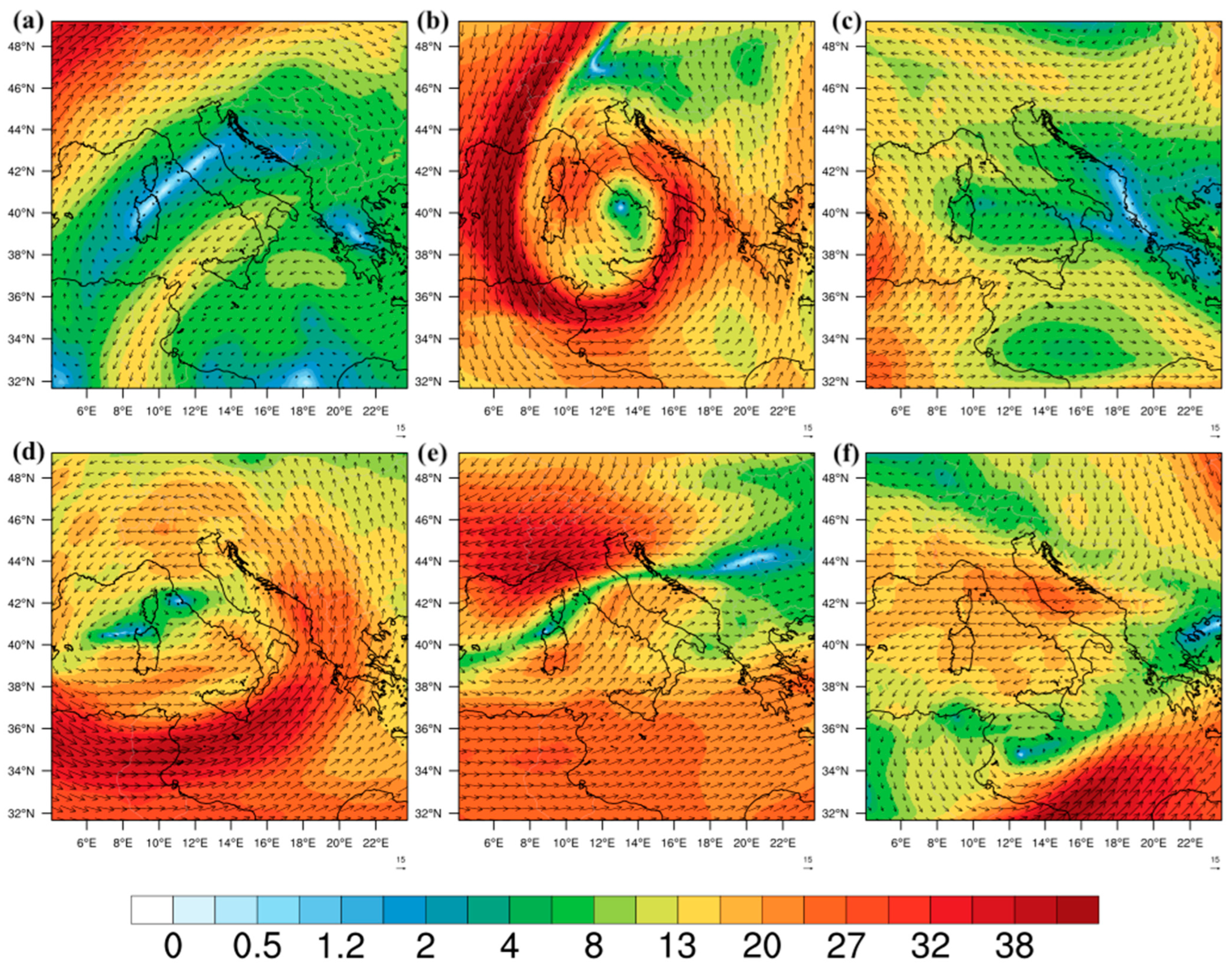
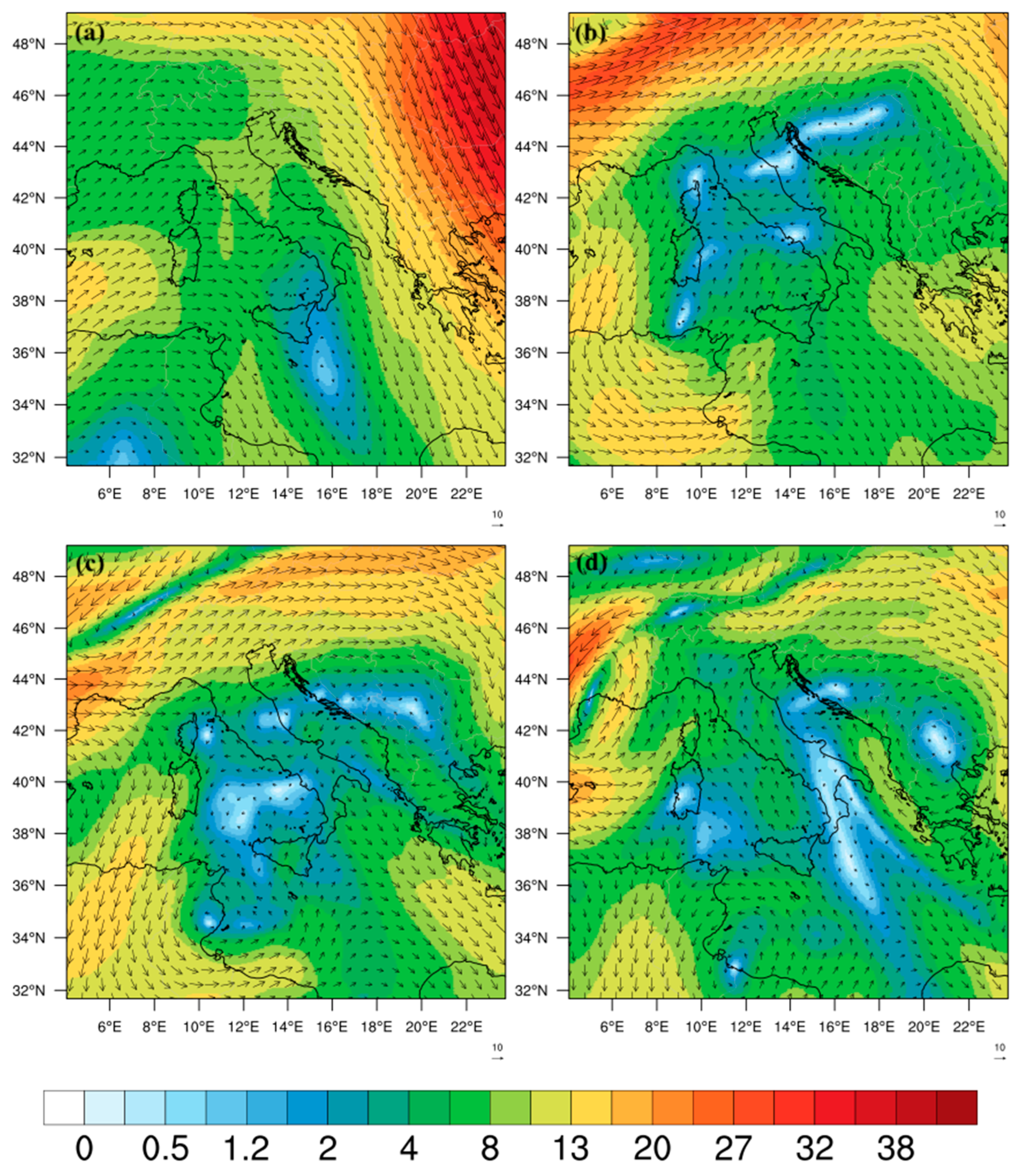
3.1. Atmospheric Circulation during the Events: Main Mid-Tropospheric Flows

In this section we describe the general synoptic situation in terms of the prevailing mid-troposphere flows, i.e., at 500 hPa, which also represents an important flight level (see next section). The geopotential height and wind vectors derived by the WRF-Chem simulations are reported in Figure 4 and Figure 5. The data are shown in correspondence with the eruption timeline for both the 2013 and the 2015 sequences; for each event, the chosen times are close to the paroxysms and are reported in

Table 5. Times of the meteorological snapshots for the synoptic analysis.

Sequence	Paroxysm	Date	UTC Time HH:MM
2013	NSE1	26 October	12:00
2013	NSE2	11 November	12:00
2013	NSE3	17 November	00:00
2013	NSE4	23 November	12:00
2013	NSE5	28 November	12:00
2013	NSE6	3 December	00:00
2015	VOR1	3 December	00:00
2015	VOR2	4 December	12:00
2015	VOR3	5 December	00:00
2015	VOR4	5 December	12:00

.

Although studied as a unique sequence, the 2013 eruptions lasted 38 days and the atmospheric configurations continually changed; it nevertheless generated some recurrent flows. For some of the six 2013 eruptive events, several similarities are in fact noticeable in terms of the synoptic configuration and prevailing upper-level winds. For NSE2, NSE4, and NSE5 (Figure 4b, Figure 4d and Figure 4e, respectively), some upper-level troughs, although of different amplitudes and depths, dominated the central Tyrrhenian, favoring south-westerly winds in southern Italy and in the Sicily region in particular.

Figure 4. WRF geopotential height [m] and wind barbs at 500 hPa for the 2013 paroxysms, namely (a) NSE1, (b) NSE2, (c) NSE3, (d) NSE4, (e) NSE5, and (f) NSE6.

Figure 4. WRF geopotential height [m] and wind barbs at 500 hPa for the 2013 paroxysms, namely (a) NSE1, (b) NSE2, (c) NSE3, (d) NSE4, (e) NSE5, and (f) NSE6.

For NSE6 (Figure 4f) a trough is also visible, but located south of the Strait of Sicily, between the southern coasts in the region and north Africa. This configuration favored the advection of south-easterly upper-level winds over eastern Sicily.

An upper-level ridge is visible in the southern Mediterranean for the NSE3 case (Figure 4c); this structure is connected to a trough in the Balearics, and the main mid-tropospheric flows over north-eastern Sicily followed the curvature of the ridge, i.e., with currents toward east-southeast.

Finally, a different (from the previous ones) configuration is noticeable for NSE1 (Figure 4a), characterized by a wide high-pressure area over the whole Italian Peninsula. In this situation, the upper-level currents over Sicily were weaker and mainly directed towards the southwest, also driven by a lower pressure area over North Africa.

For the 2015 sequence (Figure 5), that lasted about 3 days, the main synoptic configuration remained quite stationary and was characterized by a very wide high-pressure system persistently dominating the whole Mediterranean basin, only slowly moving westward during the sequence. Some local (and weak) high- and low-pressure areas, visible in Figure 5, developed over the Mediterranean during this sequence, maintaining relatively weak mid-tropospheric currents; these winds flowed over north-eastern Sicily firstly toward the east (Figure 5a,b) and later, after the formation of a local low over North Africa, toward the north (Figure 5a,b).

Figure 5. WRF geopotential height [m] and wind vectors at 500 hPa for the 2015 paroxysms, namely (a) VOR1, (b) VOR2, (c) VOR3, and (d) VOR4.

Figure 5. WRF geopotential height [m] and wind vectors at 500 hPa for the 2015 paroxysms, namely (a) VOR1, (b) VOR2, (c) VOR3, and (d) VOR4.

To highlight some general differences between the two sequences it can be seen that the 2013 eruptive events were characterized by a succession of different baric configurations, most of the time characterized by the presence of low-pressure areas over the central Mediterranean. On the contrary the 2015 events, that occurred in a few days, were characterized by a prevailing and quite stationary, wide high-pressure system, with smaller pressure gradients in the Mediterranean. The resulting circulations at 500 hPa were also quite different, with mid-tropospheric currents on average in the range 20–40 m s⁻¹ for 2013 (Figure A2) and less than 10 m s⁻¹ for the 2015 (Figure A3) sequence, respectively. These results, based on the WRF-Chem simulations, represent a robust meteorological basis for the evaluation of regional-scale ash transportation after volcanic eruptions (see next section).

3.2. Analysis of the Volcanic Ash Dispersion Patterns

The objective of this work is to evaluate the contamination of the airspace by a succession of Mount Etna explosive paroxysms and the implications for hazards, in particular, with respect to air traffic in the Mediterranean area. For this purpose, we define the vertically integrated ($\overline{p_{10}}$) mass, that is calculated considering the ash bins of the E1 distribution (Table 4) with a diameter less than 10 μm, as follows:

$$\overline{p_{10}}={\int }_0^{top}<PM10>{\rho }_{air}dz$$

(2)

$$PM10=0.5\times vash\_10+vash\_9+0.5\times vash\_8$$

(3)

where PM10 is the sum of the finest ash bins (units μg kg⁻¹) and ${\rho }_{air}$ is the density of the air (kg m⁻³). The brackets denote the time average over the simulation period and the vertical integration (represented by the overbar) is performed considering the whole vertical domain (top = 18 km). The resulting $\overline{p_{10}}$ units are expressed in μg m⁻², which can be considered as the columnar ash concentration.

The model simulations produce hazard maps for $\overline{p_{10}}$ to provide information on the atmospheric ash dispersal of PM10, but it should be remembered that the time and spatially averaged representations presented below are intended to guide aviation in terms of the hazard appraisal and risk mitigation of Etna paroxysms. These representations should not be confused with instantaneous ash concentrations that could be met by aircraft or measured by instruments at a given moment. To circumvent the lack of vertical information on the columnar ash concentration representations, we derive ash concentrations at specific flight levels in Section 3.2.2 by performing a WRF-Chem data interpolation (3D) for a given pressure level (a specialized function of the NCAR Command Language named wrf_user_intrp3d). To provide a further image of the ash dispersal with a better time resolution, in Section 3.2.3 we also compute the daily average ash concentration at specific flight levels for four selected paroxysms.

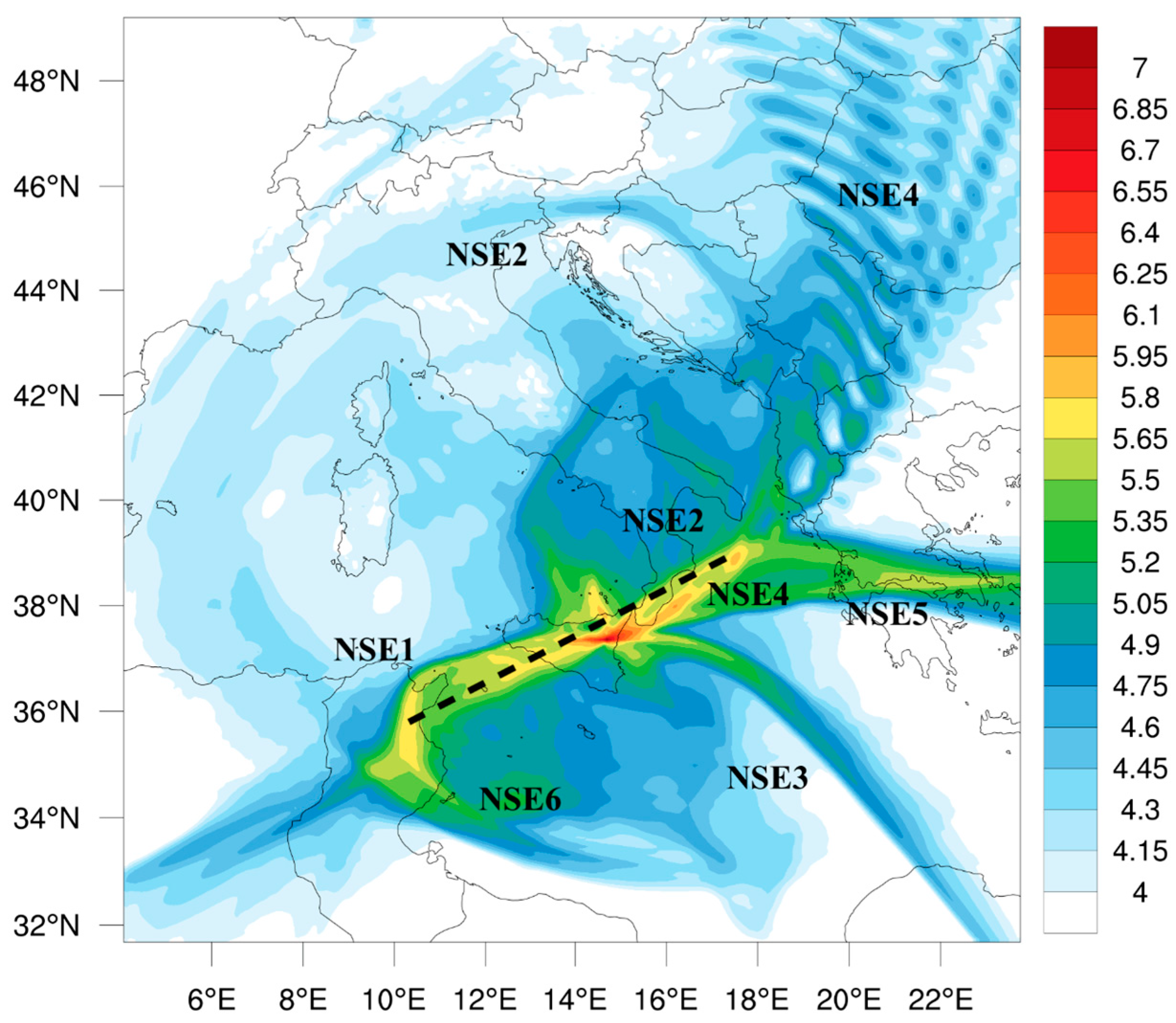
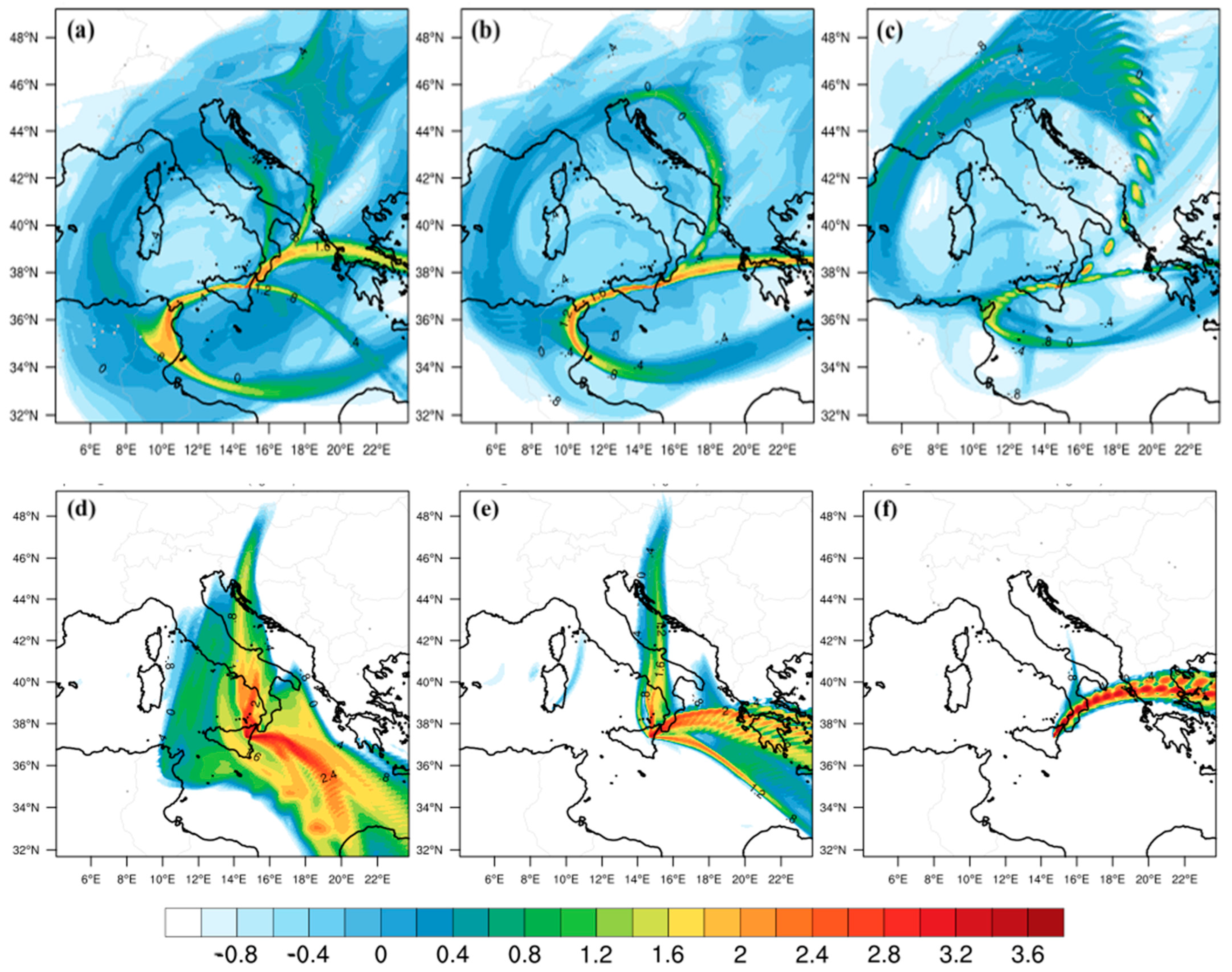
3.2.1. Time-Averaged Columnar Ash Concentration Maps

Figure 6 and Figure 7 show the results for the 2013 and the 2015 sequences, respectively. Both figures were built considering the time average for the full simulated sequences. For the 2013 sequence, a successive spatial filter is applied to leave out days without ash in the domain.

These two figures provide a quantitative estimation of the global contamination of airspace by a succession of eruptions. The average spatial pattern outlined by the 2013 sequence (Figure 6) shows, basically, three affected regions in terms of vertically integrated columnar ash concentrations: a red-shaded region around 10 g m⁻² within a radius of approximately 100 km, a yellow-shaded region in the order of 0.5 g m⁻² within a ~500 km radius, and a green/blue-shaded area with columnar ash content lower than 0.1 g m⁻² within a ~800 km radius. This average spatial pattern is overprinted by the dispersal from each event oriented by the specific wind conditions, conferring a starfish-like overall pattern. Another feature that is evident in Figure 6, is a wave-like pattern, caused by NSE4 in the northward direction. This happened because NSE4 was very rapid (3 h, see Table 1) and the most intense in the whole sequence (Figure 1d). A wave-like pattern results from the combined effect of the time-varying MER, for particularly strong and short eruptions, and the averaging (daily) of the pulsed ash plumes.

The distribution of the columnar ash concentrations from the 2015 short sequence (Figure 7) presents a similar starfish-like spatial pattern, with remarkable differences consisting of: (1) a more extensive red-shaded region centered on Sicily and south Italy and it is also more intense in terms of magnitude, within a radius of approximately 150 km from the eruptive crater, and (2) a strong eastward upper tropospheric transportation caused by the VOR1 eruption. Again, a wave-like pattern is evident in the eastward direction caused by the VOR1 paroxysm, which is the most intense in the whole sequence. As highlighted in the previous section, these differences are mainly related to the different mid-tropospheric transportation conditions during the two sequences and also by the very rapid succession of eruptive episodes in December 2015, which generated powerful eruption columns up to the stratosphere.

Additionally, in order to evaluate the influence of precipitation on the dispersion of ash, we analyzed the amount of precipitation in the domain by elaborating the Integrated Multi-satellitE Retrievals for Global Precipitation Measurement (GPM-IMERG Final Precipitation, Level 3 products), for the two periods considered in this work. The WRF-Chem model has specialized routines to calculate dry/wet deposition for aerosol components, including volcanic ash. Specifically, the “below cloud” wet deposition is handled by considering the sum of large-scale rain (from the microphysics scheme) and convective rain (by the cumulus scheme).

For the 2013 sequence, Figure A4a shows the area around Etna clear from precipitation, and 30 mm of accumulated precipitation in the Ionian and southern Adriatic seas. By comparing it with the average $\overline{p_{10}}$ map in Figure 6, the amount of ash deposited on the ground by wet deposition is arguably quite small. In the second period in December 2015, there was no rain in the domain except in the Tyrrhenian Sea close to the east coast of Sardinia (Figure A4b). By comparing it with the average $\overline{p_{10}}$ map in Figure 7, the amount of ash deposited on the ground by wet deposition may be considered negligible.

This analysis on the global contamination of the airspace by a succession of eruptions may be considered a preliminary indication of potential hazard zones around Mount Etna, which can be re-evaluated as eruption sequences in different meteorological conditions are recorded and analyzed.

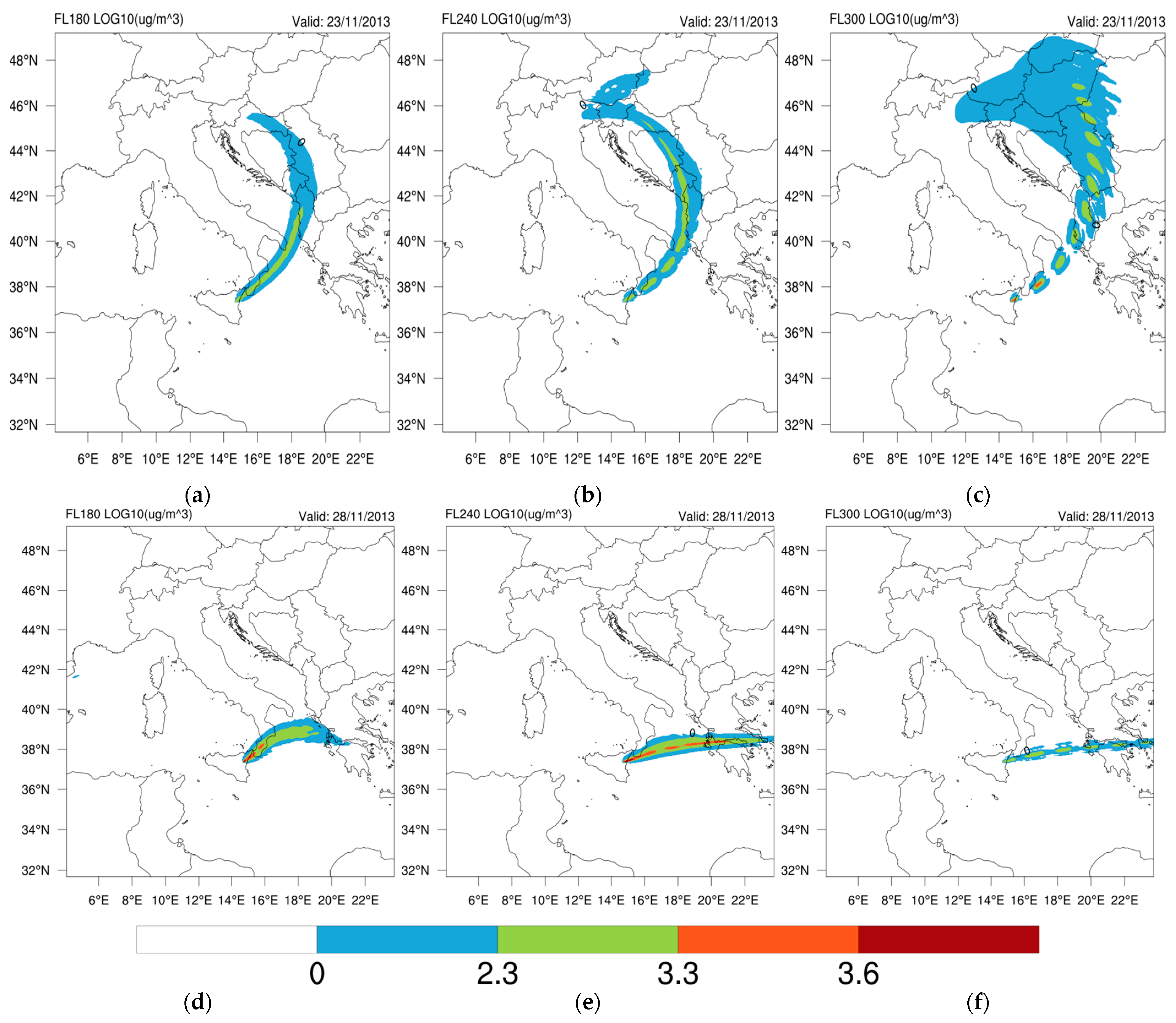
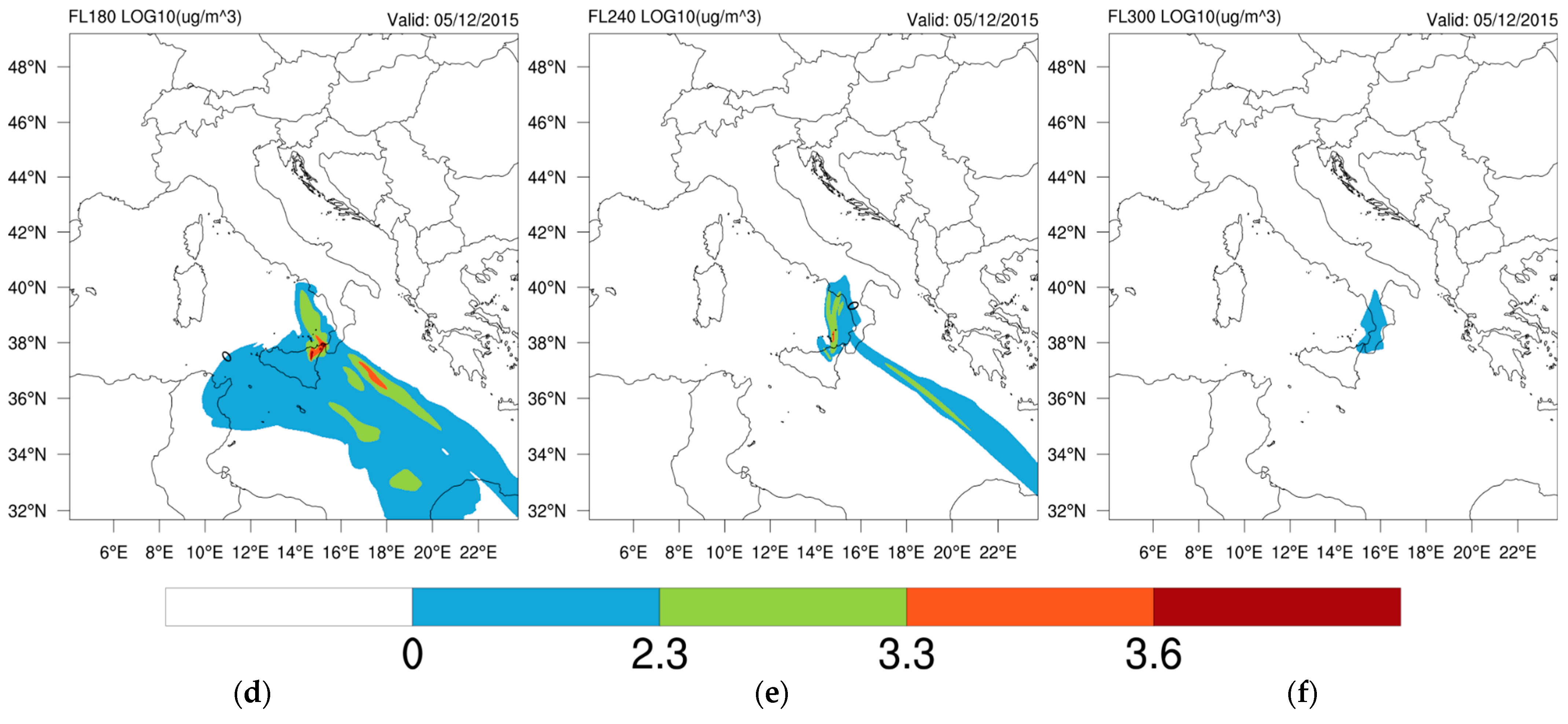
3.2.2. Time-Averaged Ash Concentration Maps at Specified Flight Levels

To evaluate the contamination of the airspace and the related hazards to aviation, it is necessary to point out that the forecasts by the VAACs (https://www.ssd.noaa.gov/VAAC/vaac.html, accessed on 8 February 2023) use the following concentration thresholds to define the ensuing levels of ash contamination: low (200–2000 μg m⁻³), medium (2000–4000 μg m⁻³), and high (>4000 μg m⁻³).

The flight level (FL), represents the altitude of an aircraft at the standard air pressure, expressed in hundreds of feet (1 FL = 100 ft). It may be considered as a proxy for elevation, and it may be associated with a given pressure level, as reported in

Table 6. Flight levels in the airspace, the corresponding pressure level, and the associated height above sea level (a.s.l.).

Pressure Level (hPa)	Flight Level (FL)	Height (Feet, a.s.l.)	Height (m, a.s.l.)
300	FL300	30,000	9200
400	FL240	24,000	7300
500	FL180	18,000	5500

. These levels correspond to the upper airspace characterized by the ICAO, as the zone where most air transport operations take place.

In Figure 8, the time-averaged PM10 concentration for the 2013 (upper row) and 2015 (bottom row) sequences is displayed, at flight levels FL180 (panels a,d), FL240 (panels b,e), and FL300 (panels c,f), corresponding to the pressure levels at 500, 400, and 300 hPa (Table 6). The label scale in Figure 8 is saturated at 4000 μg m⁻³ (corresponding to 10^3.6), which represents the threshold defined by the ICAO for a high level of contamination and the consequent prohibited airspace.

The transportation of volcanic ash at these flight levels has different patterns for each respective sequence. The effects of the low-pressure weather conditions that occurred during the 2013 sequence are particularly evident in Figure 8a–c, from the circular to the elliptical stretched vortices (800 to over 1600 km in diameter) that transported volcanic ash counter-clockwise at large distances. This is particularly evident in the 2013 sequence for FL180 (Figure 8a) and FL240 (Figure 8b) flight levels, at which ash remains concentrated mainly along these vortices in narrow bands, generally less than 100 km wide. Ash concentrations in these bands range from about 1 to over 4000 μg m⁻³. Being well localized during these high-wind conditions, ash can remain concentrated over long distances, up to 25 μg m⁻³ (10^1.4) at 1000 km eastward for the most violent paroxysm in the sequence that occurred on 23 November 2013 (NSE4). At FL300 (300 hPa) in the upper troposphere, vortices are still present, but ash is more widely dispersed in the north direction owing to tropospheric wind at 300 hPa (Figure 8c).

In contrast, the 2015 sequence, occurring in prevalently high-pressure conditions and weak winds (see Figure A3), caused high ash concentrations at all flight levels, as outlined by the red-shaded area in Figure 8d–f. At FL300 (Figure 8f), mostly the intense eastward transportation of very fine ash from VOR1 by tropospheric wind at 300 hPa is visible, due to the combination of the eruption intensity and high-pressure low-wind conditions. Considering this is a time-averaged map, this potentially indicates high ash hazards at all flight levels during, and for days following, this eruptive sequence. The concentration of very fine ash appears more localized, spatially going upward into the upper troposphere, although still reaching the no-fly zone level.

What can be inferred from this analysis on the PM10 maps at these flight levels is that long-range transportation is strictly correlated with synoptic circulation. In particular, synoptic patterns with relatively weak tropospheric currents are conditions leading to the accumulation of volcanic ash in the atmosphere after an eruption. This seems a rather obvious conclusion, but it is important to highlight the fundamental role played by the meteorological component in VATDM models and the need for their online coupling with numerical aerosol packages.

This result is in part confirmed by analyzing the VAAs issued by the Toulouse VAAC that are reported in Table A1. A total of 19 VAAs were issued in the period 3–6 December, of which 12 were classified as “Red”, 6 “Orange”, and 1 “Yellow”.

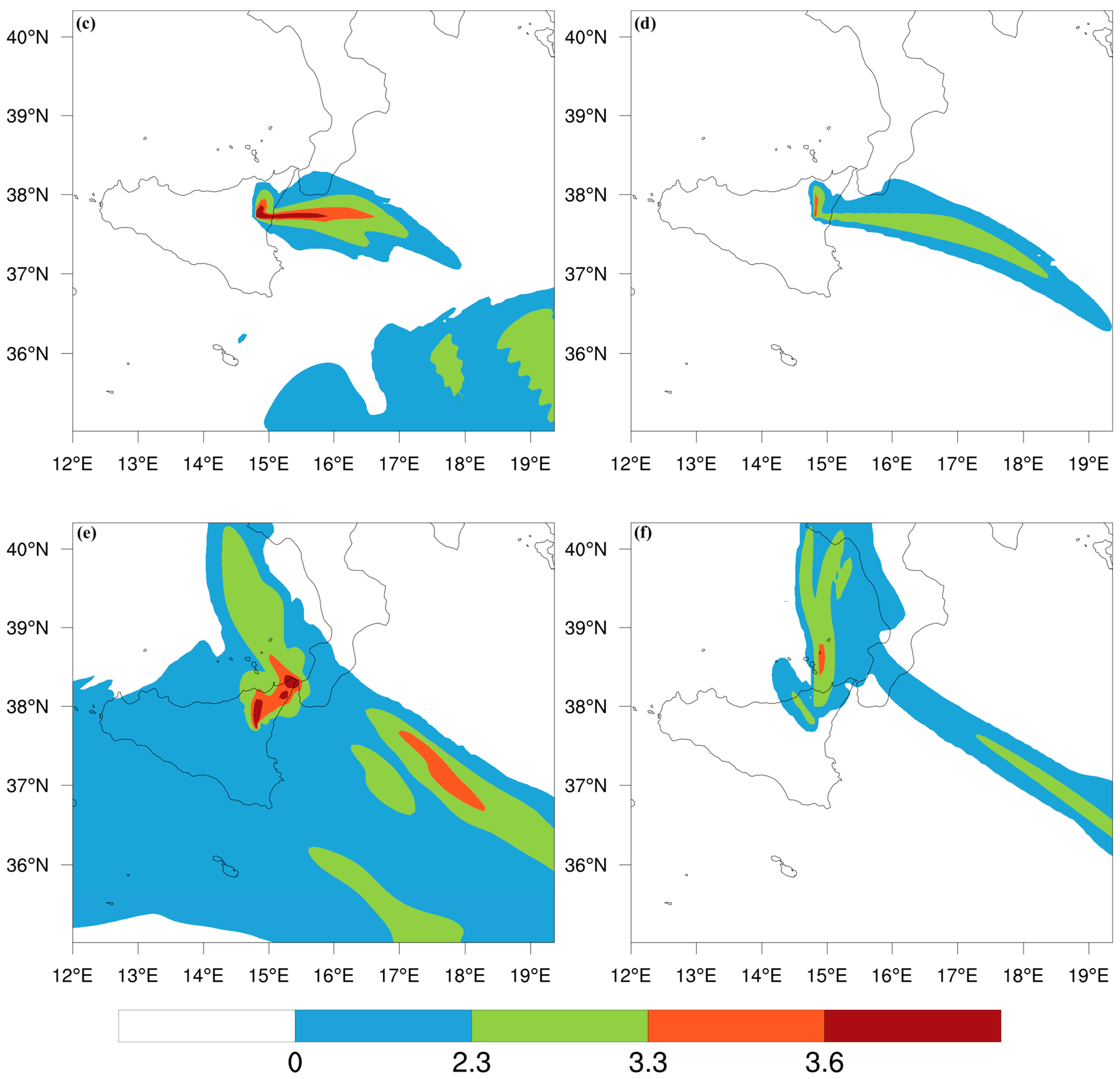
3.2.3. Daily Average Ash Concentration Maps for Selected Paroxysms

In the following, Figure 9 and Figure 10, we analyzed the daily average (from 00:00 UTC until 23:59) ash concentrations from two powerful paroxysms, with the first sequence having the most contrasted durations on November 23 (NSE4, 3.2 h) and 28 (NSE5, 8.3 h), and the most contrasted MERs for the second sequence on 3 December (VOR1) and 5 (VOR3-4). It is calculated by performing a daily time average on the selected day and reported as p_10D. The left column in both figures (panels a–d) refers to FL180, the central column to FL240 (panels b–e), and the right column to FL300 (panels c–f). The contour shading matches the above-mentioned four hazard levels used in aviation for volcanic ash concentration, reported in

Table 7. Shading intervals reported in Figure 9 and Figure 10 and their connection with the hazard levels defined by the UK Civil Aviation Authority [44] and used by the ICAO.

p10D Interval (μg m−3)	log10 Scale	Shading	Hazard Level
0–200	0–2.2	blue	none
200–2000	2.2–3.3	green	low
2000–4000	3.3–3.6	red	medium
>4000	> 3.6	dark red	high

.

For the NSE4 paroxysm, the geopotential height at 500 hPa (Figure 4d) shows a wide low-pressure area in the central Mediterranean basin, favoring south-westerly strong upper-tropospheric winds (>30 ms⁻¹) in southern Italy. The very fine ash was rapidly transported toward Albania (in about 6 h) and the Balkan regions at relatively low concentrations (Figure 9a).

The very fine ash after the NSE5 paroxysm (Figure 9d–f) was transported eastward in a straight line by the intense zonal currents at 500 hPa (Figure 4e).

These maps indicate low potential risks for aviation at FL180 to FL300. The shading contours (blue–green) indicate, in fact, the low hazard level. On the other side, all the 21 VAAs from the Toulouse VAAC reported in Table A1 indicate the “NIL” alert level (NIL = no ash cloud is produced) for the whole period.

The corresponding analysis on the 2015 sequence is depicted in Figure 10. Panels a-b-c in the upper row report the daily p_10D concentration at FL180, FL240, and FL300 for 3 December 2015 (VOR1), while the lower panels (d-e-f) describe the equivalent for 5 December 2015 (VOR3 and VOR4).

For both cases, the p_10D daily patterns, in agreement with the high-pressure meteorological conditions (Figure 5a,d), indicate a red-shaded region in the proximity of Mount Etna for FL180 and FL240 (panels a-b-c-d). FL300 (Figure 10c), relative to VOR1, again reveals the presence of a p_10D ash fraction at the upper tropospheric level (about 9200 m) in the form of a wave-like pattern, which is the artificial effect of the averaging (daily) of the pulsed ash plumes. To better visualize these maps, a high-resolution Figure A1 is provided in the Appendix A, which zooms in on the Mount Etna area. This is consistent with the 19 VAAs issued by the Toulouse VAAC during the period 3–6 December 2015, 12 of which were classified as “Red” and 6 as “Orange”.

3.2.4. Vertical Distribution of Very Fine Ash

Animated videos (gif files) (Supplementary Materials) showing the fast volcanic PM10 space–time evolution of the successive emissions (often ‘pulse-like’), due to the transient nature of their source, can be found at https://doi.org/10.25519/GG1K-2H34 (accessed on 20 June 2023) for the 2013 and 2015 sequences. Figure 11 shows extracted snapshots for different paroxysms, providing information on the vertical distribution of PM10 along the cross-sections indicated in Figure 6 and Figure 7. The ash cloud thickness is particularly valuable information for aviation hazard assessment and countermeasures in the case of an ash encounter, and for satellite mass retrievals, as generally a non-measured average thickness is assumed. For instance, the ash cloud inherited from the 26 October 2013 tephra plume (NSE1) is seen slowly drifting to the SW after about 1.5 days between 1.9 and 3.7 km a.s.l., i.e., with an inferred vertical thickness of about 1.8 km (Figure 11a). After the top part of the VOR1 plume had risen above 12 km a.s.l. in the minutes following the eruption onset, some very fine ash from the middle region of the eruptive column was observed after 7 h, rising to the NE above 11.8 km a.s.l. with an inferred vertical thickness of about 2.5–3 km (Figure 11c), while the lower part of the eruptive column fed another PM10 cloud, 700 m thick, drifting at about 2 km a.s.l. laterally to the SW 1.5 days after the onset (Figure 11d). The modelled ash cloud from the 4 December 2015 evening paroxysm had a vertical thickness of 1.4 km at an altitude of 5 km a.s.l. when the following paroxysm occurs (Figure 11f). Note that an ongoing vertical plume emission coexisting with ash from a previous plume is visible in Figure 11e,f.

Figure 11. Vertical distribution of PM10 hourly concentrations (in μg m⁻³) as a function of air pressure (in hPa, cf. corresponding heights in Table 6), altitude (i.e., from 0 to 11.8 km a.s.l.) and position, along the SW-NE transects shown in Figure 6 (panels a,b) and Figure 7 (panels c–f). Specifically, (a) 27 October 2013 at 20:00 UTC, (b) 31 October 2013 at 03:00 UTC, (c) 3 December 2015 at 11:00 UTC, (d) 4 December 2015 at 15:00 UTC, (e) 4 December 2015 at 21:00 UTC, and (f) 5 December 2015 at 15:00 UTC. The 4000 μg m⁻³ concentration corresponds to prohibited airspace. Horizontal scales are 750 km (a,b) and 900 km (c–f). The topography of Etna and Aspromonte in Calabria appear in white.

Figure 11. Vertical distribution of PM10 hourly concentrations (in μg m⁻³) as a function of air pressure (in hPa, cf. corresponding heights in Table 6), altitude (i.e., from 0 to 11.8 km a.s.l.) and position, along the SW-NE transects shown in Figure 6 (panels a,b) and Figure 7 (panels c–f). Specifically, (a) 27 October 2013 at 20:00 UTC, (b) 31 October 2013 at 03:00 UTC, (c) 3 December 2015 at 11:00 UTC, (d) 4 December 2015 at 15:00 UTC, (e) 4 December 2015 at 21:00 UTC, and (f) 5 December 2015 at 15:00 UTC. The 4000 μg m⁻³ concentration corresponds to prohibited airspace. Horizontal scales are 750 km (a,b) and 900 km (c–f). The topography of Etna and Aspromonte in Calabria appear in white.

Another interesting feature seen in Figure 11b,e is ash stagnating for several days at ground level. PM10 concentrations are common above 500 μg m⁻³, as can be seen during four days in late October to early November 2013 following NSE1. PM10 concentrations at ground level can even punctually exceed the aviation threshold, as observed following VOR2 around the occurrence time of VOR3. The repeated ash emissions from Etna, recurrently exposing the surrounding inhabitants, animals, and plants to volcanic PM10 and gas, may, therefore, potentially represent health hazards over the long term.

The timeline for ash contamination at the nearby Catania airport (CTA), or a given city, may be obtained by extrapolating the proximal ash at a given time after the onset; this would allow in-time warnings to be issued by the CTA or at any specified point in the numerical domain. This may be very important in the case where the proposed procedure goes online with an operational forecast.

4. Conclusions

We evaluate for the first time the contamination of the airspace by very fine ash from a succession of ash plumes produced by Mount Etna and the related hazards to aviation in the Mediterranean basin. To this aim, the atmospheric dispersal of sub-10 μm (PM10) ash was simulated using the WRF-Chem model coupled online with meteorology and aerosols and offline with mass eruption rates (MERs) derived from near-vent Doppler radar measurements and inferred plume altitudes. The pioneering direct input from systematic observations, best resolved in time and, thus, improving the model accuracy, is all the more valuable as paroxysms are transient and involve time-varying eruption source parameters. PM10 ash concentration hazard maps are provided for two sequences of paroxysms with widely varied volcanological conditions and contrasted occurrence interval and meteorological synoptic patterns: six ash plumes produced in 38 days during low-pressure, high-wind conditions in October–December 2013, and four ash plumes released in 3 days during high-pressure, low-wind conditions on 3–5 December 2015. The average MERs covered two orders of magnitude (2.9 × 10⁴–1.7 × 10⁶ kg s⁻¹), the durations spanned from less than 1 h to nearly half a day, and the plume top altitudes ranged from 8.1 to 13.5 km a.s.l. The synoptic conditions at 500 hPa were quite different, with mid-tropospheric current speeds on average in the range 20–40 ms⁻¹ and less than 10 ms⁻¹ for the 2013 and 2015 sequences, respectively.

We analyzed the ash PM10 dispersal in terms of time-averaged columnar ash concentration ($\underset{\_}{p_{10}}$), the concentration at specified flight levels (FL180, FL240, and FL300) averaged over the entire sequence interval (PM10), and the daily average concentration (p_10D) during selected paroxysm days at these flight levels. Consistent with the Volcanic Ash Advisories issued by the Toulouse VAAC, they may be considered as first-approach model hazard maps for aircraft and, although certainly not covering all the possible volcanological and meteorological configurations for hazard appraisal at Etna, the following conclusions can be drawn:

• The very fine ash from sequences of Mount Etna paroxysms is shown to easily contaminate the airspace around the volcano within a radius of about 1000 km in a matter of days. The airspace in many countries around the Mediterranean basin is impacted, including most of southern Europe from the Balearic Islands westward, the south of France, the whole of Italy, Greece, and the western coast of Turkey and the Balkans eastward, to beyond the Alps northward, and to Malta and the African northern coast (from Algeria to Libya) southward.
• Low-pressure weather systems favor the trapping and circulation of very fine ash in the whole troposphere within this area, yet at a low concentration, generally below 1 μg m⁻³. In this meteorological context, high winds tend to stretch ash clouds into ~100 km wide clouds forming large-scale vortices of 800–1600 km in diameter, where PM10 ash concentrations can still exceed the aviation hazard threshold up to 1000 km downwind from the volcano, a distance reached in about 10 h (e.g., NSE5).
• High-pressure, low-wind conditions tend to favor the accumulation of PM10 ash in a wide atmospheric region surrounding Etna. In this context, closely interspersed paroxysms tend to accumulate very fine ash, more diffusively in the lower troposphere and in stretched ash clouds higher up in the troposphere.
• In all the volcanological and meteorological configurations simulated, the lower troposphere appears particularly prone to the accumulation of diffuse PM10 ash during sequences of eruption; this is likely to affect the take-off and landing of aircraft in regional airports in particular.
• High MER paroxysms propel ash up into the upper troposphere, where most of the air traffic occurs, and sometimes also into the lower stratosphere, according to the weather conditions. High-troposphere ash clouds from Etna appear as a pulsed feature resulting mostly from the short-lived climax phase.
• Daily average PM10 tropospheric ash concentrations commonly exceed the aviation hazard threshold, up to 1000 km downwind from the volcano and up to the upper troposphere for intense paroxysms.
• The thickness of the modelled PM10 ash clouds generated from different parts of the eruptive columns ranged from 0.7 to 3 km.
• Potential health hazards may stem from the stagnation of PM10 ash at ground level for several days, commonly above 500 μg m⁻³, and sometimes punctually exceeding the aviation threshold. Our methodology has the potential to issue timely alerts in an operational setup, including at Catania airport.

Improving the accuracy of ash dispersal models is necessary both for nowcasting and forecasting purposes and to compensate for ash detection gaps in monitoring systems. Future WRF-Chem model developments will include refining the injection heights and the initial columnar ash distribution. The semi-empirical law from Mastin et al. [35]’s dataset used in our study averages all the observed ash plume heights from mainly large silicic explosive eruptions that have occurred in a variety of wind conditions, tending to overestimate the height from a given MER (Freret-Lorgeril et al. [20]; Figure 7). Other models relating to the MER and plume height advantageously consider the vertical wind profile (e.g., Degruyter and Bonadonna [34]). Wind profiles may come from meteorological data online coupled with WRF-Chem and cross-checked with atmospheric balloon measurements achieved several times a day in the region around Etna. Additional datasets for wind profiles at high resolution (30 km) could be considered, such as ERA5 data available from the Climate Data Store in NetCDF format [45]. Plume heights controlled by wind conditions specific to the eruption could, thus, be systematically computed from the radar-derived MER and compared with new compiled observational datasets relating to the MER and plume height (IVESPA) [14], even including discrimination of the height of the plume regions (top height, spreading level) and the SO₂ height [46]. This would lead to a more accurate definition of the injection height in the simulations.

As for future research on volcanic ash forecasts, multi-model multi-source term ensemble approaches seem to represent a promising development, as explored for instance by Plu et al. [47]. They suggest that quantiles of ash concentrations can be relevant products for air traffic management, that can be used for route optimization in the areas where ash does not pose a direct and urgent threat to aviation. Cost and disruption to air traffic could be eliminated to a great extent by including the results from dispersion models into flight planning software to apply cost-based trajectory optimizations.

References

1. Prata, F.; Rose, B. Volcanic ash hazards to aviation. In The Encyclopedia of Volcanoes, 2nd ed.; Sigurdsson, H., Ed.; Academic Press: Cambridge, MA, USA; Elsevier: Amsterdam, The Netherlands, 2015; pp. 911–934. [Google Scholar] [CrossRef]
2. International Civil Aviation Organization (ICAO). Flight Safety and Volcanic Ash, 2012. Doc 9974, ANB/487. Available online: https://www.icao.int/publications/Documents/9974_en.pdf (accessed on 10 February 2023).
3. Jiménez-Escalona, J.C.; Poom-Medina, J.L.; Roberge, J.; Aparicio-García, R.S.; Avila-Razo, J.E.; Huerta-Chavez, O.M.; Da Silva, R.F. Recognition of the Airspace Affected by the Presence of Volcanic Ash from Popocatepetl Volcano Using Historical Satellite Images. Aerospace 2022, 9, 308. [Google Scholar] [CrossRef]
4. Marchese, F.; Falconieri, A.; Filizzola, C.; Pergola, N.; Tramutoli, V. Investigating Volcanic Plumes from Mt. Etna Eruptions of December 2015 by Means of AVHRR and SEVIRI Data. Sensors 2019, 19, 1174. [Google Scholar] [CrossRef] [PubMed] [Green Version]
5. Eychenne, J.; Gurioli, L.; Damby, D.; Belville, C.; Schiavi, F.; Marceau, G.; Szczepaniaks, C.; Blavignacs, C.; Laumonier, M.; Gardes, E.; et al. Spatial distribution and physicochemical properties of respirable volcanic ash from the 16-17 August 2006 Tungurahua eruption (Ecuador), and alveolar epithelium response in-vitro. GeoHealth 2022, 6, e2022GH000680. [Google Scholar] [CrossRef]
6. Sellitto, P.; Salerno, G.; Corradini, S.; Xueref-Remy, I.; Riandet, A.; Bellon, C.; Khaykin, S.; Ancellet, G.; Lolli, S.; Welton, E.J.; et al. Volcanic emissions, plume dispersion, and downwind radiative impacts following Mount Etna series of eruptions of February 21–26, 2021. J. Geophys. Res. Atmos. 2023, 128, e2021JD035974. [Google Scholar] [CrossRef]
7. EUROCONTROL. 11 Years after the Eruption of Icelandic Volcano Eyjafjallajökull. Available online: https://www.eurocontrol.int/news/11-years-after-eruption-icelandic-volcano-eyjafjallajokull (accessed on 23 June 2023).
8. Hirtl, M.; Arnold, D.; Baro, R.; Brenot, H.; Coltelli, M.; Eschbacher, K.; Hard-Stremayer, H.; Lipok, F.; Maurer, C.; Meinhard, D.; et al. A volcanic-hazard demonstration exercise to assess and mitigate the impacts of volcanic ash clouds on civil and military aviation. Nat. Hazards Earth Syst. Sci. 2020, 20, 1719–1739. [Google Scholar] [CrossRef]
9. Guffanti, M.; Casadevall, T.J.; Budding, K. Encounters of Aircraft with Volcanic Ash Clouds: A Compilation of Known Incidents, 1953–2009: U.S. Geological Survey Data Series, 2010, 545, Ver. 1.0, 12 p., Plus 4 Appendixes Including the Compilation Database. Available online: https://pubs.usgs.gov/ds/545/ (accessed on 14 February 2023).
10. Christmann, C.; Nunes, R.R.; Schmitt, A.R. Recent Encounters of Aircraft with Volcanic Ash Clouds. Deutscher Luft-und Raumfahrtkongress (DLR), 2015, DocumentID: 370124. Available online: https://www.dglr.de/publikationen/2015/370124.pdf (accessed on 14 February 2023).
11. Thouret, J.-C.; Charbonnier, S. Assessment, Delineation of Hazard Zones and Modeling of Volcanic Hazards. In Hazards and Monitoring of Volcanic Activity 1; Lénat, J.-F., Ed.; ISTE-Géosciences: Lausanne, Switzerland, 2022; pp. 151–184. ISBN 978-1-78945-043-9. [Google Scholar] [CrossRef]
12. Folch, A. A review of tephra transport and dispersal models: Evolution, current status, and future perspectives. J. Volcanol. Geotherm. Res. 2012, 235–236, 96–115. [Google Scholar] [CrossRef]
13. Harvey, N.J.; Huntley, N.; Dacre, H.F.; Goldstein, M.; Thomson, D.; Webster, H. Multi-level emulation of a volcanic ash transport and dispersion model to quantify sensitivity to uncertain parameters. Nat. Hazards Earth Syst. Sci. 2018, 18, 41–63. [Google Scholar] [CrossRef] [Green Version]
14. Aubry, T.J.; Engwell, S.; Bonadonna, C.; Carazzo, G.; Scollo, S.; Van Eaton, A.R.; Taylor, I.A.; Jessop, D.; Eychenne, J.; Gouhier, M.; et al. The Independent Volcanic, Eruption Source Parameter Archive (IVESPA, versio 1.0): A new observational database to support explosive eruptive column model validation and development. J. Volcanol. Geotherm. Res. 2021, 417, 107295. [Google Scholar] [CrossRef]
15. Egan, S.D.; Stuefer, M.; Webley, P.W.; Lopez, T.; Cahill, C.F.; Hirtl, M. Modeling volcanic ash aggregation processes and related impacts on the April–May 2010 eruptions of Eyjafjallajökull volcano with WRF-Chem. Nat. Hazards Earth Syst. Sci. 2020, 20, 2721–2737. [Google Scholar] [CrossRef]
16. Grell, G.A.; Peckham, S.E.; Schmitz, R.; McKeen, S.A.; Frost, G.; Skamarock, W.C.; Eder, B. Fully coupled “online” chemistry within the WRF model. Atmos. Environ. 2005, 39, 6957–6976. [Google Scholar] [CrossRef]
17. Rizza, U.; Brega, E.; Caccamo, M.T.; Castorina, G.; Morichetti, M.; Munaò, G.; Passerini, G.; Magazù, S. Analysis of the ETNA 2015 Eruption Using WRF–Chem Model and Satellite Observations. Atmosphere 2020, 11, 1168. [Google Scholar] [CrossRef]
18. Rizza, U.; Donnadieu, F.; Magazu, S.; Passerini, G.; Castorina, G.; Semprebello, A.; Morichetti, M.; Virgili, S.; Mancinelli, E. Effects of Variable Eruption Source Parameters on Volcanic Plume Transport: Example of the 23 November 2013 Paroxysm of Etna. Remote Sens. 2021, 13, 4037. [Google Scholar] [CrossRef]
19. Donnadieu, F.; Freville, P.; Hervier, C.; Coltelli, M.; Scollo, S.; Prestifilippo, M.; Valade, S.; Rivet, S.; Cacault, P. Near-source Doppler radar monitoring of tephra plumes at Etna. J. Volcanol. Geotherm. Res. 2016, 312, 26–39. [Google Scholar] [CrossRef]
20. Freret-Lorgeril, V.; Donnadieu, F.; Scollo, S.; Provost, A.; Fréville, P.; Guéhenneux, Y.; Hervier, C.; Prestifilippo, M.; Coltelli, M. Mass Eruption Rates of Tephra Plumes during the 2011–2015 Lava Fountain Paroxysms at Mt. Etna From Doppler Radar Retrievals. Front. Earth Sci. 2018, 6, 73. [Google Scholar] [CrossRef]
21. Bonaccorso, A.; Calvari, S.; Linde, A.; Sacks, S. Eruptive processes leading to the most explosive lava fountain at Etna volcano: The 23 November 2013 episode. Geophys. Res. Lett. 2014, 41, 4912–4919. [Google Scholar] [CrossRef]
22. Poret, M.; Corradini, S.; Merucci, L.; Costa, A.; Andronico, D.; Montopoli, M.; Vulpiani, G.; Freret-Lorgeril, V. Reconstructing volcanic plume evolution integrating satellite and ground-based data: Application to the 23 November 2013 Etna eruption. Atmos. Chem. Phys. Discuss. 2018, 18, 4695–4714. [Google Scholar] [CrossRef] [Green Version]
23. Corradini, S.; Guerrieri, L.; Lombardo, V.; Merucci, L.; Musacchio, M.; Prestifilippo, M.; Scollo, S.; Silvestri, M.; Spata, G.; Stelitano, D. Proximal Monitoring of the 2011–2015 Etna Lava Fountains Using MSG-SEVIRI Data. Geosciences 2018, 8, 140. [Google Scholar] [CrossRef] [Green Version]
24. Corsaro, R.A.; Andronico, D.; Behncke, B.; Branca, S.; Caltabiano, T.; Ciancitto, F.; Cristaldi, A.; De Beni, E.; La Spina, A.; Lodato, L.; et al. Monitoring the December 2015 summit eruptions of Mt. Etna (Italy): Implications on eruptive dynamics. J. Volcanol. Geotherm. Res. 2017, 341, 53–69. [Google Scholar] [CrossRef]
25. Crafford, A.E.; Venzke, E. (Eds.) Global Volcanism Program. Report on Etna (Italy). In Bulletin of the Global Volcanism Network; Smithsonian Institution: Washington, DC, USA, 2017; Volume 42, p. 5. [Google Scholar] [CrossRef]
26. Bonaccorso, A.; Calvari, S. A new approach to investigate an eruptive paroxysmal sequence using camera and strainmeter networks: Lessons from the 3–5 December 2015 activity at Etna volcano. Earth Planet. Sci. Lett. 2017, 475, 231–241. [Google Scholar] [CrossRef]
27. Bonforte, A.; Cannavo, F.; Gambino, S.; Guglielmo, F. Combining High- and Low-Rate Geodetic Data Analysis for Unveiling Rapid Magma Transfer Feeding a Sequence of Violent Summit Paroxysms at Etna in Late 2015. Appl. Sci. 2021, 11, 4630. [Google Scholar] [CrossRef]
28. Donnadieu, F.; Freret-Lorgeril, V.; Gouhier, M.; Coltelli, M.; Scollo, S.; Fréville, P.; Hervier, C.; Prestifilippo, M. The 3 December 2015 paroxysm of Voragine crater at Etna: Insights from Doppler radar measurements. Geophys. Res. Abstr. 2016, 18, EGU2016-17201-1. [Google Scholar]
29. Dubosclard, G.; Donnadieu, F.; Allard, P.; Cordesses, R.; Hervier, C.; Coletllie, M.; Privitera, E.; Kornprobst, J. Doppler radar sounding of volcanic eruption dynamics at Mount Etna. Bull. Volcanol. 2004, 66, 443–456. [Google Scholar] [CrossRef]
30. Marzano, F.S.; Mereu, L.; Scollo, S.; Donnadieu, F.; Bonadonna, C. Tephra Mass Eruption Rate from X-Band and L-Band Microwave Radars during the 2013 Etna Explosive Lava Fountain. IEEE Trans. Geosci. Remote Sens. 2020, 58, 3314–3327. [Google Scholar] [CrossRef]
31. Freret-Lorgeril, V.; Bonadonna, C.; Corradini, S.; Donnadieu, F.; Guerrieri, L.; Lacanna, G.; Marzano, F.; Mereu, L.; Merucci, L.; Ripepe, M.; et al. Examples of Multi-Sensor Determination of Eruptive Source Parameters of Explosive Events at Mount Etna. Remote Sens. 2021, 13, 2097. [Google Scholar] [CrossRef]
32. Mereu, L.; Scollo, S.; Bonadonna, C.; Donnadieu, F.; Freret-Lorgeril, V.; Marzano, F.S. Ground-Based Remote Sensing and Uncertainty Analysis of the Mass Eruption Rate Associated With the 3–5 December 2015 Paroxysms of Mt. Etna. IEEE J. Sel. Top. Appl. Earth Obs. Remote Sens. 2022, 15, 504–518. [Google Scholar] [CrossRef]
33. Donnadieu, F.; Freville, P.; Rivet, S.; Hervier, C.; Cacault, P. The Volcano Doppler Radar Data Base of Etna (VOLDORAD-2B); Université Clermont Auvergne CNRS: Clermont-Ferrand, France, 2015. [Google Scholar] [CrossRef]
34. Degruyter, W.; Bonadonna, C. Improving on mass flow rate estimates of volcanic eruptions. Geophys. Res. Lett. 2012, 39, L16308. [Google Scholar] [CrossRef] [Green Version]
35. Mastin, L.G.; Guffanti, M.; Servranckx, R.; Webley, P.; Barsotti, S.; Dean, K.; Durant, A.; Ewert, J.W.; Neri, A.; Rose, W.I.; et al. A multidisciplinary effort to assign realistic source parameters to models of volcanic ash-cloud transport and dispersion during eruptions. J. Volcanol. Geotherm. Res. 2009, 186, 10–21. [Google Scholar] [CrossRef]
36. Stuefer, M.; Freitas, S.R.; Grell, G.; Webley, P.; Peckham, S.; McKeen, S.A.; Egan, S.D. Inclusion of ash and SO2 emissions from volcanic eruptions in WRF-Chem: Development and some applications. Geosci. Model Dev. 2013, 6, 457–468. [Google Scholar] [CrossRef] [Green Version]
37. Shi, J.J.; Matsui, T.; Tao, W.K.; Tan, Q.; Peters-Lidard, C.; Chin, M.; Pickering, K.; Guy, N.; Lang, S.; Kemp, E.M. Implementation of an aerosol–cloud-microphysics–radiation coupling into the NASA unified WRF: Simulation results for the 6–7 August 2006 AMMA special observing period. Q. J. R. Meteorol. Soc. 2014, 140, 2158–2175. [Google Scholar] [CrossRef] [Green Version]
38. Rizza, U.; Avolio, E.; Morichetti, M.; Di Liberto, L.; Bellini, A.; Barnaba, F.; Virgili, S.; Passerini, G.; Mancinelli, E. On the Interplay between Desert Dust and Meteorology Based on WRF-Chem Simulations and Remote Sensing Observations in the Mediterranean Basin. Remote Sens. 2023, 15, 435. [Google Scholar] [CrossRef]
39. Janjic, Z.I. The Step–Mountain Eta Coordinate Model: Further developments of the convection, viscous sublayer, and turbulence closure schemes. Mon. Weather Rev. 1994, 122, 927–945. [Google Scholar] [CrossRef]
40. Janjic, Z.I. The surface layer in the NCEP Eta Model. In Proceedings of the Eleventh Conference on Numerical Weather Prediction, Norfolk, VA, USA, 19–23 August 1996; pp. 354–355. [Google Scholar]
41. Niu, G.-Y.; Yang, Z.-L.; Mitchell, K.E.; Chen, F.; Ek, M.B.; Barlage, M.; Kumar, A.; Manning, K.; Niyogi, D.; Rosero, E.; et al. The community Noah land surface model with multiparameterization options (Noah–MP): 1. Model description and evaluation with local–scale measurements. J. Geophys. Res. 2011, 116, D12109. [Google Scholar] [CrossRef] [Green Version]
42. Chou, M.D.; Suarez, M.J. A solar radiation parameterization for atmospheric studies. NASA Tech. Memo. 1999, 15, 40. [Google Scholar]
43. Lang, S.E.; Tao, W.K.; Chern, J.D.; Wu, D.; Li, X. Benefits of a fourth ice class in the simulated radar reflectivities of convective systems using a bulk microphysics scheme. J. Atmos. Sci. 2014, 71, 3583–3612. [Google Scholar] [CrossRef]
44. UK Civil Aviation Authority: CAP1236: Guidance Regarding Flight Operations in the Vicinity of Volcanic Ash, 33 pp. 2017. Available online: https://publicapps.caa.co.uk/docs/33/CAP%201236%20FEB17.pdf (accessed on 21 May 2023).
45. Climate Data Store. Available online: https://cds.climate.copernicus.eu/#!/home (accessed on 4 September 2022).
46. Aubry, T.J.; Engwell, S.L.; Bonadonna, C.; Mastin, L.G.; Carazzo, G.; Van Eaton, A.R.; Jessop, D.E.; Grainger, R.G.; Scollo, S.; Taylor, I.A.; et al. New insights into the relationship between mass eruption rate and volcanic column height based on the IVESPA data set. Geophys. Res. Lett. 2023, 50, e2022GL102633. [Google Scholar] [CrossRef]
47. Plu, M.; Scherllin-Pirscher, B.; Arnold Arias, D.; Baro, R.; Bigeard, G.; Bugliaro, L.; Carvalho, A.; El Amraoui, L.; Eschbacher, K.; Hirtl, M.; et al. An ensemble of state-of-the-art ash dispersion models: Towards probabilistic forecasts to increase the resilience of air traffic against volcanic eruptions. Nat. Hazards Earth Syst. Sci. 2021, 21, 2973–2992. [Google Scholar] [CrossRef]
Figure 3. The injection height from Equation (1) [35]. Violet points: 2013 sequence; green points: 2015 sequence. Units for MER are kg s−1.
Remotesensing 15 03760 g003
Figure 6. Average distribution of the total columnar p 10 ¯ ash concentration related to the 2013 paroxysms. Data without ash in the domain are filtered out. Units are in μg m−2 and reported in the log10 scale. The dotted line denotes the cross-section transect depicted in Figure 11a,b.
Remotesensing 15 03760 g006
Figure 7. Average distribution of the total columnar p 10 ¯ ash concentration related to the 2015 paroxysms. Units are in μg m−2 and reported in the log10 scale. The dotted line denotes the cross-section transect depicted in Figure 11c–f.
Remotesensing 15 03760 g007
Figure 8. Top (ac): time-averaged PM10 concentration maps for the October–December 2013 sequence at different flight levels, namely (a) FL180, (b) FL240, and (c) FL300. Bottom (df): time-averaged PM10 concentration maps for the December 2015 sequence at the same flight levels as in a,b,c. Units are in μg m−3 and are reported in the log10 scale. The upper scale limit of 4000 μg m−3 (3.6 in log10 scale) corresponds to prohibited airspace.
Remotesensing 15 03760 g008
Figure 9. Daily average p10D ash concentrations at different flight levels for 23 November 2013 (first row); 28 November 2013 (second row). Panels (a,d) for FL180; panels (b,e) for FL240, and panels (c,f) for FL300. Units are in μg m−3, the label bar is reported in the log10 scale with intervals matching the hazard levels for aviation.
Remotesensing 15 03760 g009
Figure 10. Daily average p10D concentrations at different flight levels for 3 December 2015 (first row); 5 December (second row). Panels (a,d) for FL180; panels (b,e) for FL240, and panels (c,f) for FL300. Units are in μg m−3, the label bar is reported in the log10 scale with intervals matching the hazard levels for aviation.
Remotesensing 15 03760 g010aRemotesensing 15 03760 g010b