Adaptive Slicing-Aided Hyper Inference for Small Object Detection in High-Resolution Remote Sensing Images

Abstract

In the field of object detection, deep learning models have achieved great success in recent years. Despite these advances, detecting small objects remains difficult. Most objects in aerial images have features that are a challenge for traditional object detection techniques, including small size, high density, high variability, and varying orientation. Previous approaches have used slicing methods on high-resolution images or feature maps to improve performance. However, existing slicing methods inevitably lead to redundant computation. Therefore, in this article we present a novel adaptive slicing method named ASAHI (Adaptive Slicing Aided Hyper Inference), which can dramatically reduce redundant computation using an adaptive slicing size. Specifically, ASAHI focuses on the number of slices rather than the slicing size, that is, it adaptively adjusts the slicing size to control the number of slices according to the image resolution. Additionally, we replace the standard non-maximum suppression technique with Cluster-DIoU-NMS due to its improved accuracy and inference speed in the post-processing stage. In extensive experiments, ASAHI achieves competitive performance on the VisDrone and xView datasets. The results show that the mAP50 is increased by 0.9% and the computation time is reduced by 20–25% compared with state-of-the-art slicing methods on the TPH-YOLOV5 pretrained model. On the VisDrone2019-DET-val dataset, our mAP50 result is 56.4% higher, demonstrating the superiority of our approach.

1. Introduction

In recent years, object detection has received much attention due to its widespread applications in various fields. When applied to images from nature, traditional object detectors such as RetinaNet [1], YOLOV5, and Fast-RCNN [2] have achieved impressive results. However, their results are not satisfactory for drone-captured and remote sensing images. For example, Faster R-CNN [3], a classical two-stage object detection algorithm, achieves 38.0 mAP on objects from the VisDrone2019 evaluation set with various sizes, but only 6.2 and 20.0 mAP, respectively, on objects with tiny and small sizes. This limitation is mainly caused by three factors: (1) low-resolution features in the deeper layer may not match the diverse size of small objects; (2) qualities such as high densities, large numbers of objects, variable scales, and small occupied areas cause significant challenges; and (3) detecting small objects is more difficult compared with large objects, as the Intersection over Union (IoU) metric can fail to account for situations such as overlapping objects, close proximity between objects, and diverse aerial perspectives.

To tackle these problems, specialized small object detection algorithms have been developed. With the appearance of 4K cameras and civilian drones and the fast development of deep learning and remote sensing technologies, the performance of small object detection using convolutional neural networks (CNNs) has substantially improved. Several methods, such as TPH-YOLOV5, TOOD [4], PP-YOLOE [5], UAVs, and SODNet [6] have obtained impressive results and are widely employed in tasks such as geographical surveys [7], person identification [8], flow monitoring [9], and traffic control. Most of these tasks require processing of high-resolution images. Hence, a number of researchers have attempted to increase the upsampling rate to maintain high-resolution features, for example, in algorithms such as TPH-YOLOV5 [10] and QueryDet [11]. Meanwhile, adding penalty terms in the post-processing stage can help to tackle problems associated with high densities. Several post-processing methods, such as Soft-NMS [12], WBF [13], and DIoU-NMS [14], have shown effectiveness in terms of improved performance. In addition, the slicing method [15] and the shifted window-based self-attention mechanism [16] have been proposed; these approaches slice images into smaller patches to amplify their local features. Both of these slicing methods have been widely used in small object detection algorithms to achieve better performance [10,11,15]. However, the redundant computations of the traditional slicing method remain, increasing computational costs and reducing detection speed. Thus, in this work our approach focuses on alleviating redundant problems to obtain better accuracy and faster detection speed when employing a small object detection algorithm on remote sensing images.

In this paper, we propose a novel slicing method, ASAHI (Adaptive Slicing-Aided Hyper Inference), which adaptively slices images into a fixed number of patches rather than using a fixed slicing size. By automatically controlling the number of slices, our method greatly reduces redundant computation. In the post-processing stage, we substitute non-maximum suppression (NMS) with Cluster-DIoU-NMS, which reduces the time consumption while maintaining the quality of the results. This approach was motivated by two key observations. First, in SAHI [15], we found that a fixed slice size leads to different degrees of redundant calculation for images with different resolutions. In particular, at the edge of the image, the redundant calculation rate exceeds the overlapping rate. By contrast, adaptive slicing size is preferable. Second, small object detection most contend with the difficulties posed by close proximity, overlap, and occlusion. NMS is a mainstream post-processing method that is widely used for object detection; however, it does not perform well for high-density objects due to its reliance on a single metric, namely, IoU. This limitation is evident in small object detection. Therefore, combining Cluster-NMS [17] and DIoU-NMS [14] is a good scheme.

We evaluated ASAHI on a challenging dataset, VisDrone2019 [18], which contains a large quantity of small objects in different resolutions. In addition, we tested it on the xView [19] dataset, which is annotated with bounding boxes and contains large amounts of aerial imagery and complex scenes from around the world. Large-scale experiments show that our method accelerates the inference and post-processing stages by 20–25%, while improving the detection performance by 2.1% compared with the baseline SAHI method [15]. 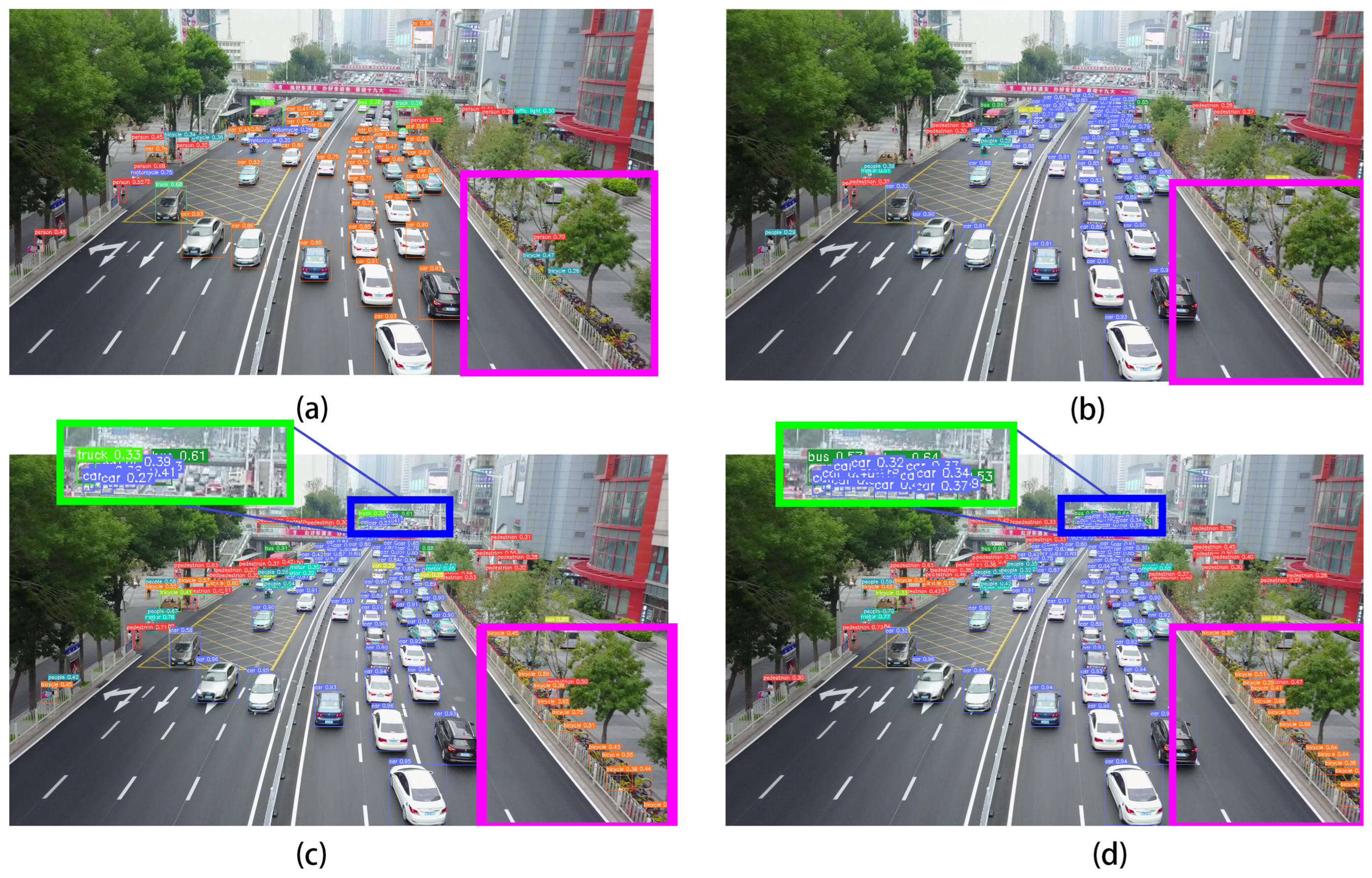Figure 1 shows the improved results obtained by ASAHI.

The main contributions of this paper are as follows:

• We propose a novel slicing method, ASAHI, which can improve detection performance for images of various resolutions and targets at a range of scales by solving the redundancy problems in the previous SAHI method [15].
• We combine ASAHI with the TPH-YOLOV5 framework [10] to strengthen its sensitivity to the lower features in deeper layers.
• We design an adaptive slicing-aided fine-tuning scheme called ASAF for data augmentation, which is more suitable for ASAHI than other traditional fine-tuning strategies.
• We integrate Cluster-DIoU-NMS, a faster Cluster-NMS method with DIoU penalty, in the post-processing stage to improve the accuracy and detection speed of inferences in high-density scenarios.

2. Related Work

Object Detection. The recent CNN-based object detectors can be divided into two main types, namely, single-stage detectors and two-stage detectors. Single-stage detectors, such as YOLOv3 [20], SSD [21], RetinaNet [1], EfficientDet [22], and YOLOV4 [23], directly predict the location of the targets; single-stage detection can be regarded as a regression problem. Two-stage detection tends to use the RoIAlign operation [24] to align an object’s features explicitly. Several typical frameworks, such as R-CNN [25], SPPNet [26], DetectoRS [27], and FPN [28], utilize a region proposal stage to generate candidate objects and selectively search those parts of an image that have a high probability of belonging to an object. Typically, single-stage detectors are less computationally expensive, while two-stage detectors achieve higher accuracy. However, the performance gap between these two approaches has narrowed recently. For example, YOLOV5 is a classical single-stage detector that uses the CSPDarknet53 architecture, with an SPP layer as the backbone and PANet as the neck. During inference, large numbers of bounding boxes are obtained and then aggregated by CIoU in the post-processing stage. This approach has attracted the attention of researchers because of its convenience and good performance.

Small Object Detection. Small object detection is a challenging task in computer vision due to the difficulties posed by low resolution, high density, variable scales, and small occupation areas. A number of researchers have modified the traditional object detection algorithms with self-attention mechanism such as CBAM [29], SPANet [30] and RTANet [31] to accommodate small object detection. An excellent work is TPH-YOLOV5 [10]; a state-of-the-art small object detection framework based on YOLOV5, it integrates an additional prediction head for small object detection, a CBAM [29] framework in the neck, and replaces the original CSP bottleneck blocks with transformer encoder blocks. This increases the detection accuracy for small objects while preserving the speed of inference. Hence, in this work we utilize TPH-YOLOV5 [10] as our backbone and propose ASAHI to achieve better results.

Postprocessing in Small Object Detection. Post-processing is a crucial part of small object detection. During the inference process, a large number of bounding boxes are generated; however, many of them represent detections of the same target, and a post-processing method must be used to suppress these false detections. In recent years, the DETR method [32] has replaced the traditional post-processing process; however, the development of this technology is not yet complete. In this paper, we maintain the use of post-processing. NMS is one of the most popular post-processing methods. Several well-known frameworks, such as TPH-YOLOV5 [10] and SAHI [15], use NMS in the post-processing stage. Although, NMS is competitive, it has a number of shortcomings due to IoU being the only influence factor in NMS. Thus, adding penalty terms is an efficient way to improve performance or reduce time consumption. For example, GIoU, DIoU, and CIoU add penalties based on the weight of non-overlapping areas, the center point distance between bounding boxes, and the aspect ratio, respectively, to improve detection performance. In addition, several methods have been combined with NMS to achieve better performance in the post-processing stage, such as IBS [33], a state-of-the-art two-stage algorithm with excellent performance, Soft-NMS [12], a soft improvement based on NMS with Gaussian algorithm, and Cascade R-CNN + NWD [34], a classical improved algorithm based on the normalized Wasserstein distance. Our method, ASAHI, focuses on better performance and faster inference. Inspired by LD [35], we employed a combination of the Cluster-NMS and DIoU-NMS [14] algorithms to meet our goals.

3. The Proposed Method

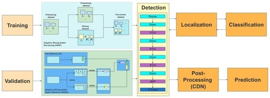
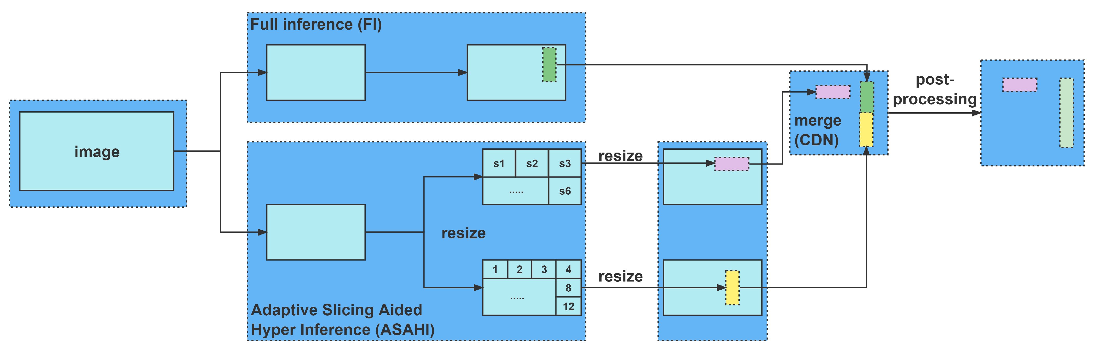
In this paper, with the aim of enhancing small object detection accuracy, we propose a novel slicing method called ASAHI, an overview of which is shown in Figure 2. The overall process can be simplified as follows: two strategies, full inference (FI) and ASAHI, are applied to the original images simultaneously. In FI, the full images are sent to the inference stage. By contrast, ASAHI adaptively changes the slicing size to control the number of slices according to the image resolution. In the inference stage, the full image and sliced image are processed by TPH-YOLOV5 [10] to obtain the corresponding bounding boxes. Next, the bounding boxes are resized by the aspect ratio and merged using Cluster-DIoU-NMS to remove the repeatedly identified pre-selected boxes in the post-processing stage. In the remainder of this section, we introduce ASAHI, Cluster-DIoU-NMS, and Adaptive Slicing Aided Fine-tuning (ASAF) in detail.

3.1. Overview of TPH-YOLOV5

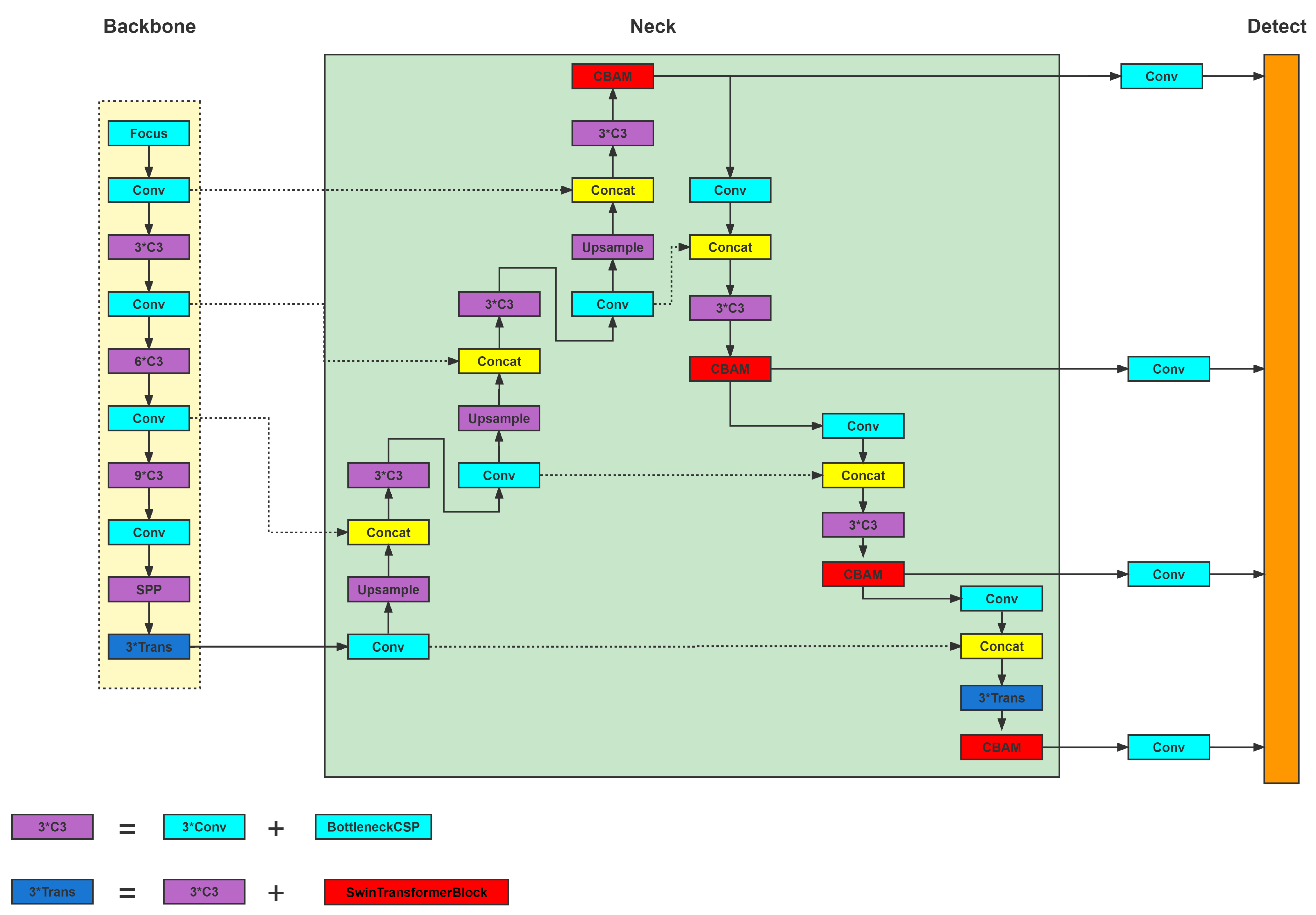
TPH-YOLOV5 [10] provides two pre-trained models, yolov5l-xs-1 and yolov5l-xs-2, which were trained at different sizes after resizing. TPH-YOLOV5 [10] uses the architecture of CSPDarknet53, with three transformer encoder blocks as the backbone, PANet with CBAM [29] as the neck, and four transformer prediction heads. Considering its excellent performance, ranking fifth in the VisDrone 2021 competition, we selected it as our backbone. Thanks to the code provided by the authors of the study [10], we used a slight modification in the neck, as shown in Figure 3, in which the number of CBAM blocks [29] is reduced by one.

3.2. Adaptive Slicing-Aided Hyper Inference (ASAHI)

By investigating a range of slicing methods, we found that fixed slice sizes inevitably lead to redundant computation in images with different resolutions. When a fixed slice size cannot be used exactly, part of the information from the previous image is included to ensure that the slice is complete; this strategy causes redundant computation, and can pose a problem for merging during post-processing. Our ASAHI approach, as an improved version of the SAHI slicing algorithm, greatly reduces this redundant computation by adaptively changing the slicing size.

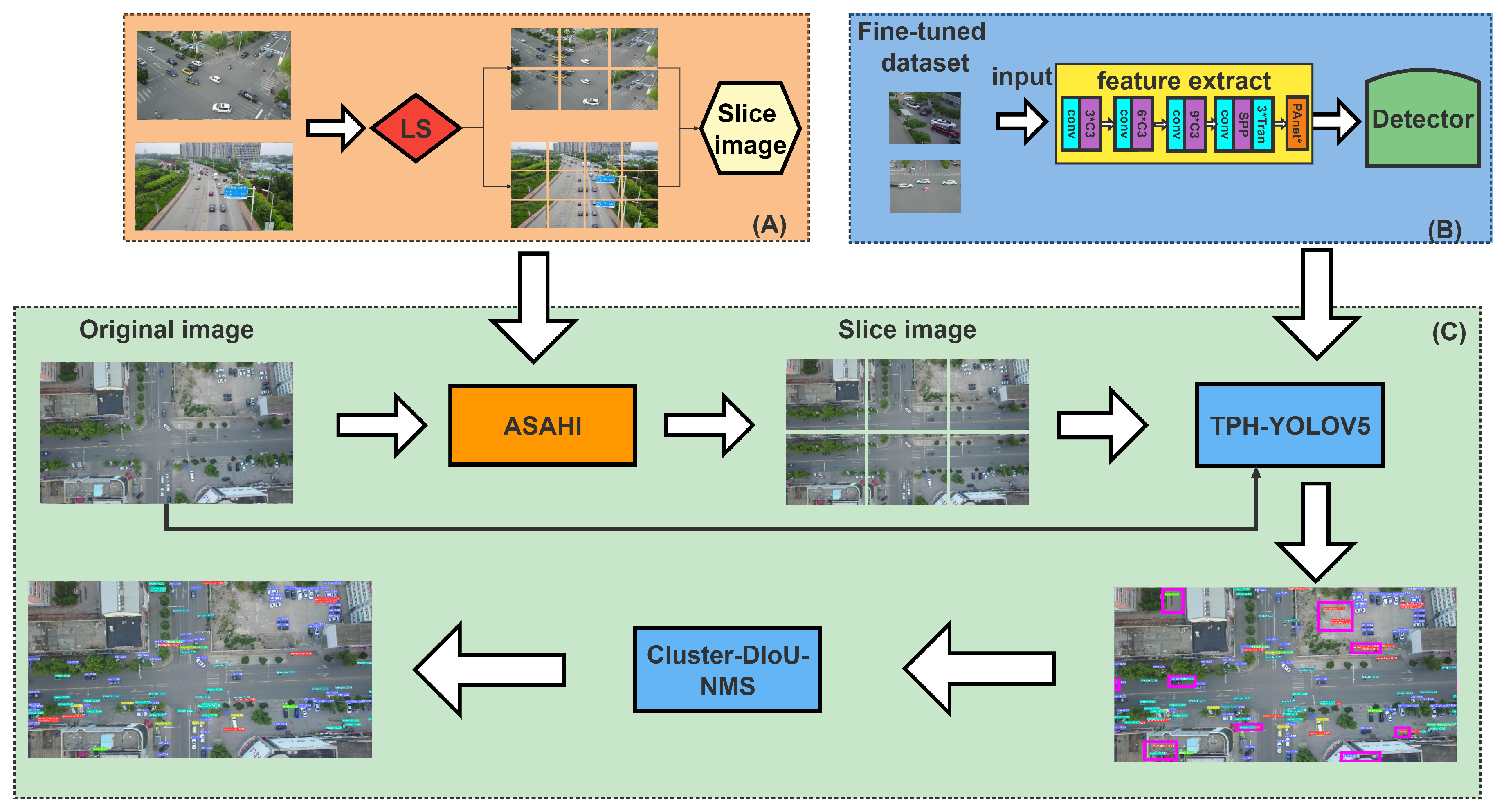
During the inference step, as detailed in Figure 4, the original image is sliced into 6 or 12 overlapping patches according to the image size. Then, each patch is resized, preserving the aspect ratio. After that, the patches are transferred to the merge stage. However, as this form of slicing results in clear defects in the detection of large objects, we use FI to detect the larger objects. Finally, Cluster-DIoU-NMS is used to merge the FI results in order to return them to their original size.

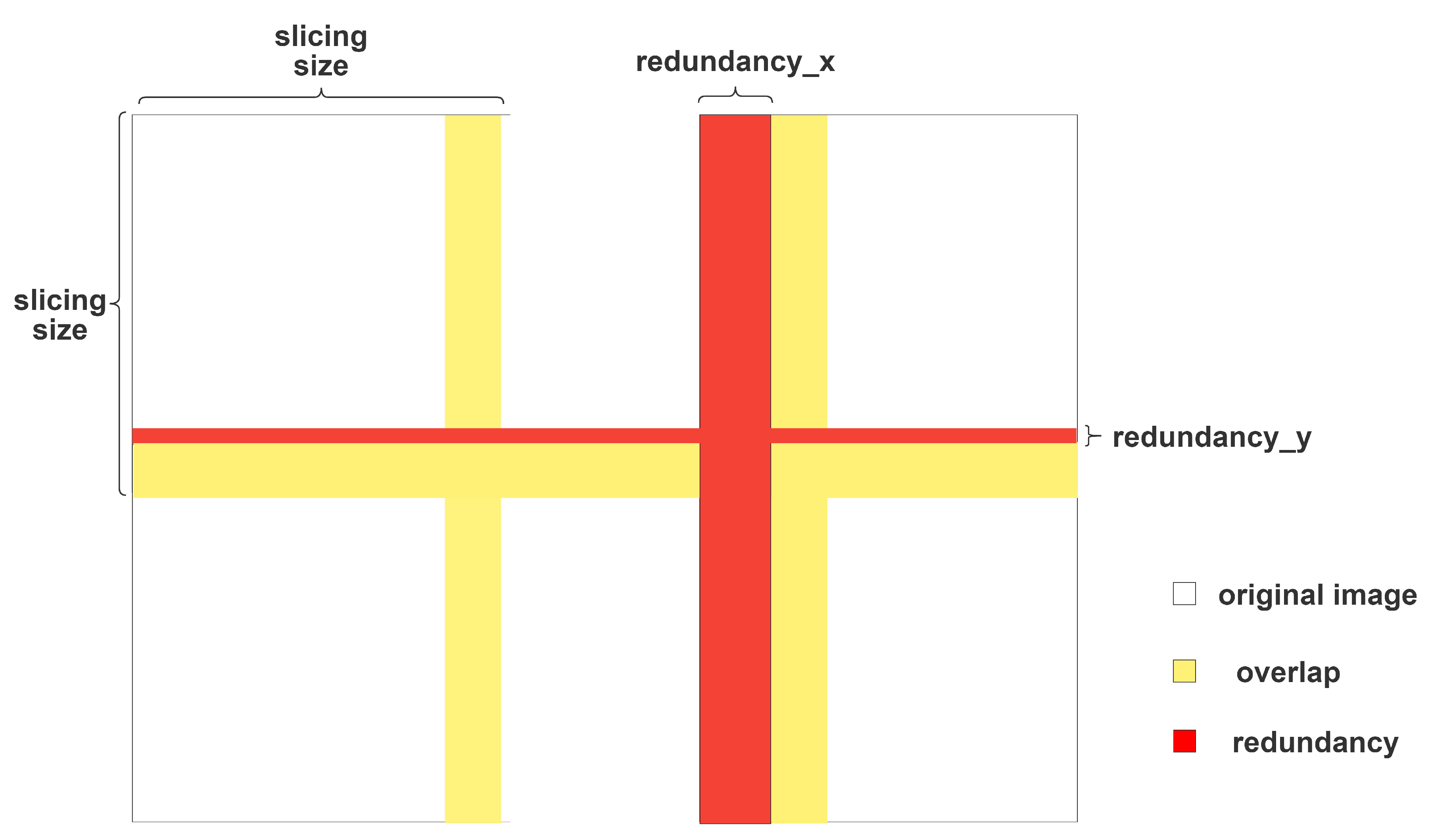
The redundancy in the inference process is shown in Figure 5, in which W and H are the length and width of the input image, respectively, and l represents the overlapping ratio. In our experiments, we noticed that the performance, as measured by the mAP, decreases if the slice sizes are different in length and width. Hence, our method maintains the same slice size in terms of length and width.

In ASAHI, we set a differentiation threshold as LS: if the length or width of the image is larger than this threshold, then the image is cut into 12 patches; otherwise, it is cut into 6 patches. LS can be calculated according to Equation (1) below. We define the restricted slice size, denoted as restrict_size, to guarantee the slice size fluctuation within restrict_size; here we set it to 512.

$$LS=\mathrm{restrict}\_\mathrm{size}·(4-3l)+1.$$

(1)

After setting the value of LS, we make sure that our image will be divided into exactly 6 and 12 patches by calculating two extreme cases and taking the maximum value:

$$p=\left\{\begin{array}{cc}max(W/(3-2l)+1,H/(2-l)+1)\hfill & max(W,H)\le \mathit{LS}\hfill \\ max(W/(4-3l)+1,H/(3-2l)+1)\hfill & max(W,H)\ge \mathit{LS}.\hfill \end{array}\right.$$

(2)

Then, we let a be the number of slices on the horizontal axis and b the number of slices on the vertical axis. They can be calculated as follows:

$$a=⌈\left(\frac{W-pl}{p\ast (1-l)}\right)⌉,$$

(3)

$$b=⌈\left(\frac{H-pl}{p(1-l)}\right)⌉.$$

(4)

We can then calculate the redundant areas in Figure 5 from the three known values of W, H, l, and p in Equation (2), as follows:

$$S_{\mathrm{area}}=WH$$

(5)

$$\mathrm{Redundancy}\_\mathrm{x}=pa-pl(a-1)-W,$$

(6)

$$\mathrm{Redundancy}\_\mathrm{y}=pb-pl(b-1)-H,$$

(7)

$$S_{\mathrm{redundancy}}=\mathrm{Redundancy}\_\mathrm{x}·H+\mathrm{Redundancy}\_\mathrm{y}·W-\mathrm{Redundancy}\_\mathrm{x}·\mathrm{Redundancy}\_\mathrm{y}.$$

(8)

After calculating the redundancy of the ASAHI method, we can derive the reduction in redundant computational area compared to the SAHI [15] method as follows:

$$S_{\mathrm{redundancy}}^{\mathrm{ASAHI}}=\left\{\begin{array}{cc}W\left(p\right(2-l)-H)\hfill & \frac{W}{(3-2l)}\ge \frac{H}{(2-l)}\&max(W,H)\le \mathit{LS}\hfill \\ H\left(p\right(3-2l)-W)\hfill & \frac{W}{(3-2l)}<\frac{H}{(2-l)}\&max(W,H)\le \mathit{LS}\hfill \\ W\left(p\right(3-2l)-H)\hfill & \frac{W}{(4-3l)}\ge \frac{H}{(3-2l)}\&max(W,H)>\mathit{LS}\hfill \\ H\left(p\right(4-3l)-W)\hfill & \frac{W}{(4-3l)}<\frac{H}{(3-2l)}\&max(W,H)>\mathit{LS}\hfill \end{array}\right.$$

(9)

$$S_{\mathrm{Reduction}}^{\mathrm{Time}}=1-(S_{\mathrm{redundancy}}^{\mathrm{ASAHI}}+S_{\mathrm{area}})/(S_{\mathrm{redundancy}}+S_{\mathrm{area}})$$

(10)

The redundant computation generated by SAHI [15] is decreased through our method. The proportions of the reduced redundant computation for images of various resolutions are shown in

Table 1. Reduction in the redundancy of the computed area with ASAHI as compared to SAHI [15] at different resolutions. All image resolutions are from the VisDrone and xView [19] datasets.

Image Resolution	Redundant Calculation Reduction (%)
$960\times 540$	38.72
$1360\times 765$	2.56
$1400\times 1050$	25.61
$1920\times 1080$	25.92
$2000\times 1500$	24.13
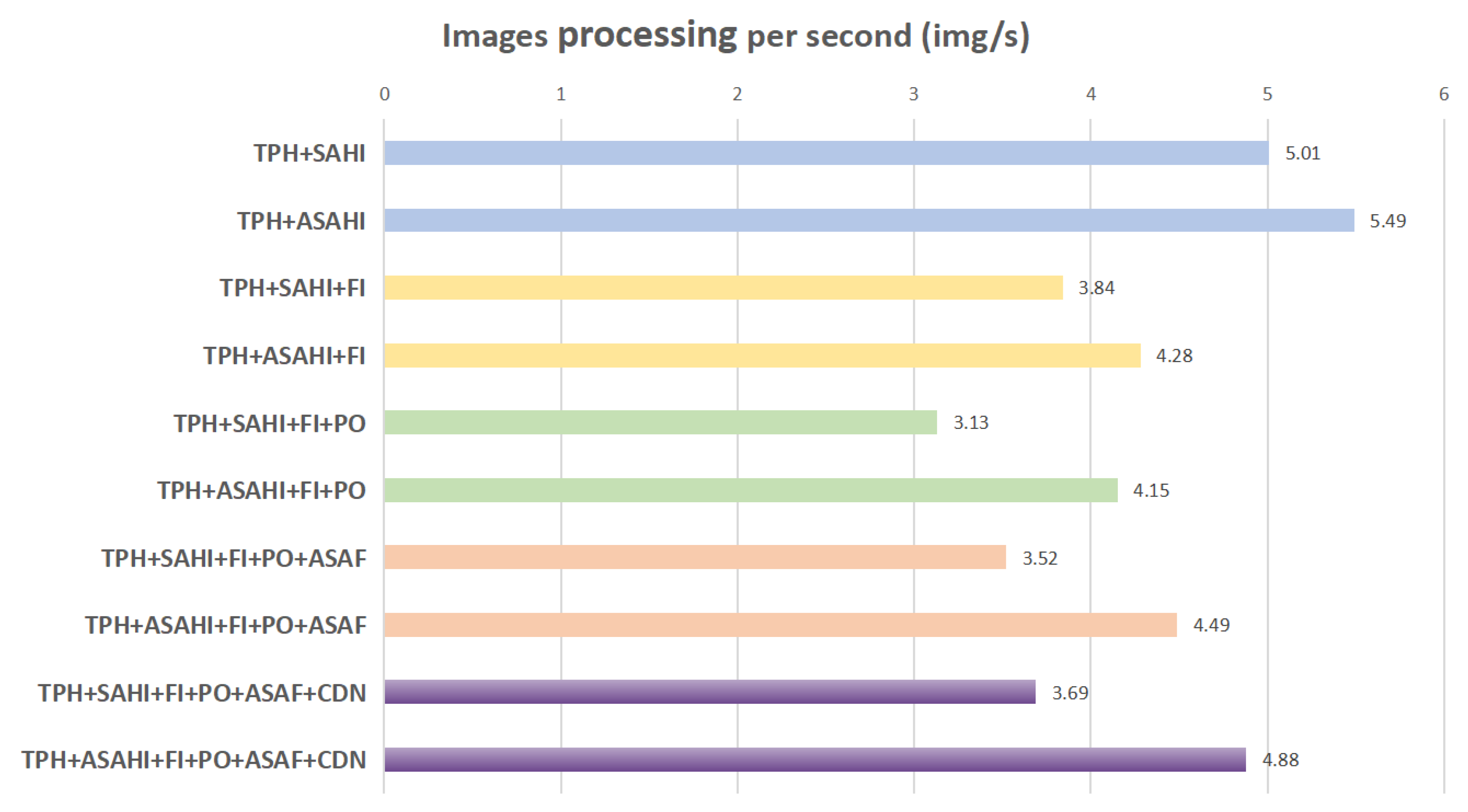
$2913\times 2428$	6.99

. As a result of this reduction, ASAHI is able to achieve improved processing speed.

3.3. Cluster-DIoU-NMS

Post-processing is a crucial part of small object detection. Inspired by LD [35], we employed Cluster-DIoU-NMS in the post-processing stage due to the outstanding performance of Cluster-NMS [17] and DIoU-NMS [14]. Briefly, Cluster-DIoU-NMS is a combination of DIoU-NMS [14] and Cluster-NMS [17]. We used the structure of Cluster-NMS in order to speed up the detection speed, and replaced the IOU metric with DIoU to improve performance in overlapping scenarios. In other words, the oversuppression issue is addressed by Cluster-NMS and the DIoU parameters are employed to strengthen the accuracy.

DIoU-NMS: In the traditional NMS algorithm, IoU is the only factor considered. However, in practical applications it is difficult to distinguish objects by IoU alone when the distance between two objects is small. Therefore, the overlapping area of the two bounding boxes and the distance of the center point should be considered simultaneously in post-processing; despite this, traditional IoU only takes the overlapping area into account, ignoring the centroid distance. To address this issue, DIoU-NMS [14] incorporates the distance between the center points of the two boxes as a penalty term. If the IoU between two boxes is relatively large and the distance between the centers is relatively small, the boxes are deemed to be separate objects and are not filtered out. In DIoU, $c^2$ denotes the diagonal distance of the smallest wrapped box overlaying the two bounding boxes, while ${\rho }^2(x,x^{gt})$ represents the Euclidean distance between the centroids of the two boxes. DIoU is defined as

$$\mathrm{DIoU}=\mathrm{IoU}-\frac{{\rho }^2(x,x^{gt})}{c^2}.$$

(11)

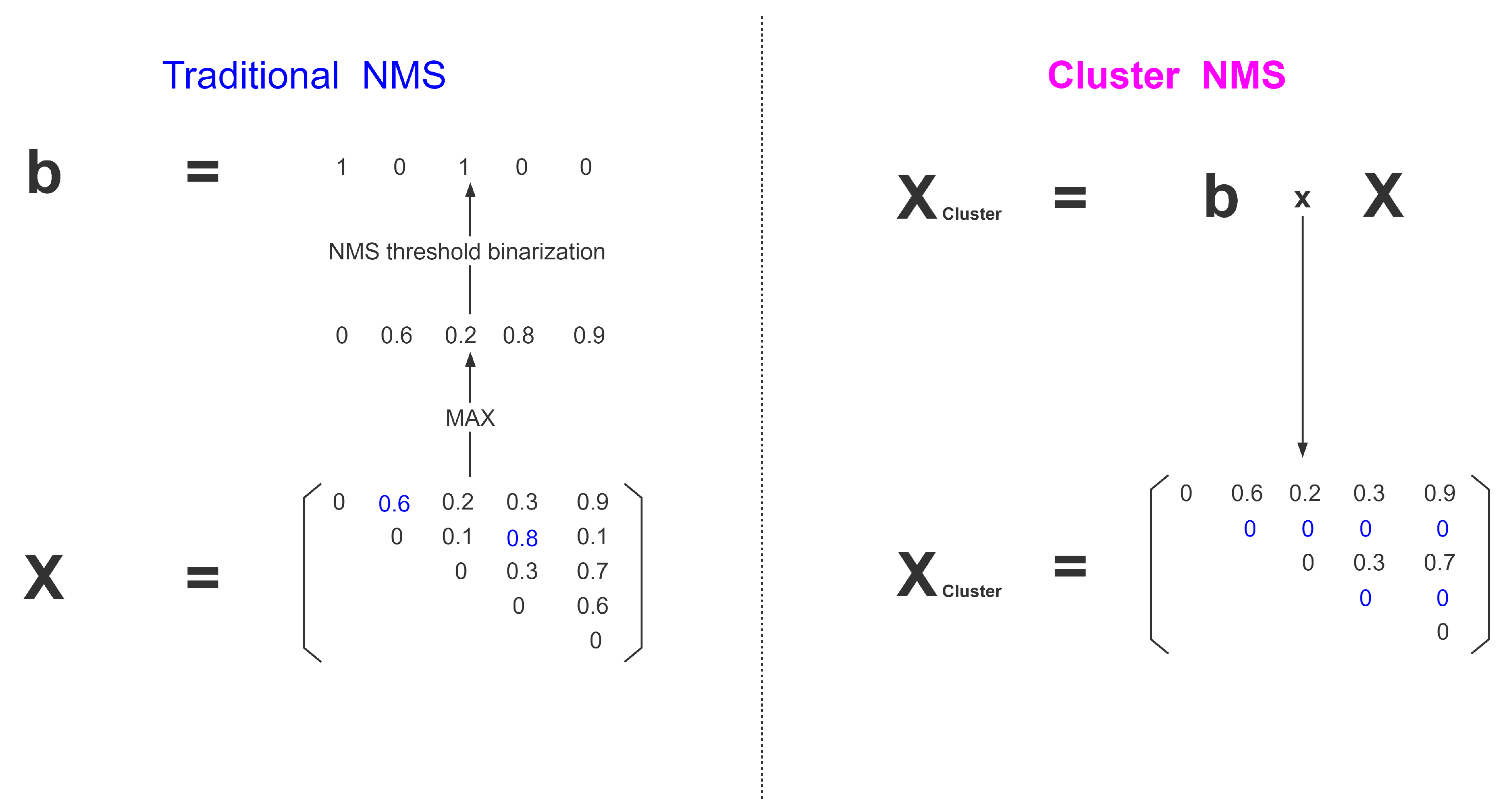
Cluster-NMS: In traditional NMS, as shown in the left of Figure 6, the matrix $\mathbf{X}$ consists of i rows and j columns, which are sorted by score and upper triangulation, and each element $X_{ij}$ represents the computed IoU of the ith bbox and the jth bbox. Then, the maximum value is taken for each column and binarized to obtain the resulting sequence $\mathbf{b}$. However, in the blue part of Figure 6, 0.6 is calculated from the first and second bbox; the IoU exceeds the threshold, and should be suppressed. The first bbox and the second bbox should be considered as one box. Therefore, the bbox in the fourth column of the second row should be excluded, which is computed by the second and fourth bbox. This means that 0.8 should not appear. In contrast, Cluster-NMS employs a simple and effective alteration. Before binarization, $X_{Cluster}$ multiplies $\mathbf{b}$ to the left by $\mathbf{X}$, which can solve the over-inhibition problem, as shown in the right of Figure 6.

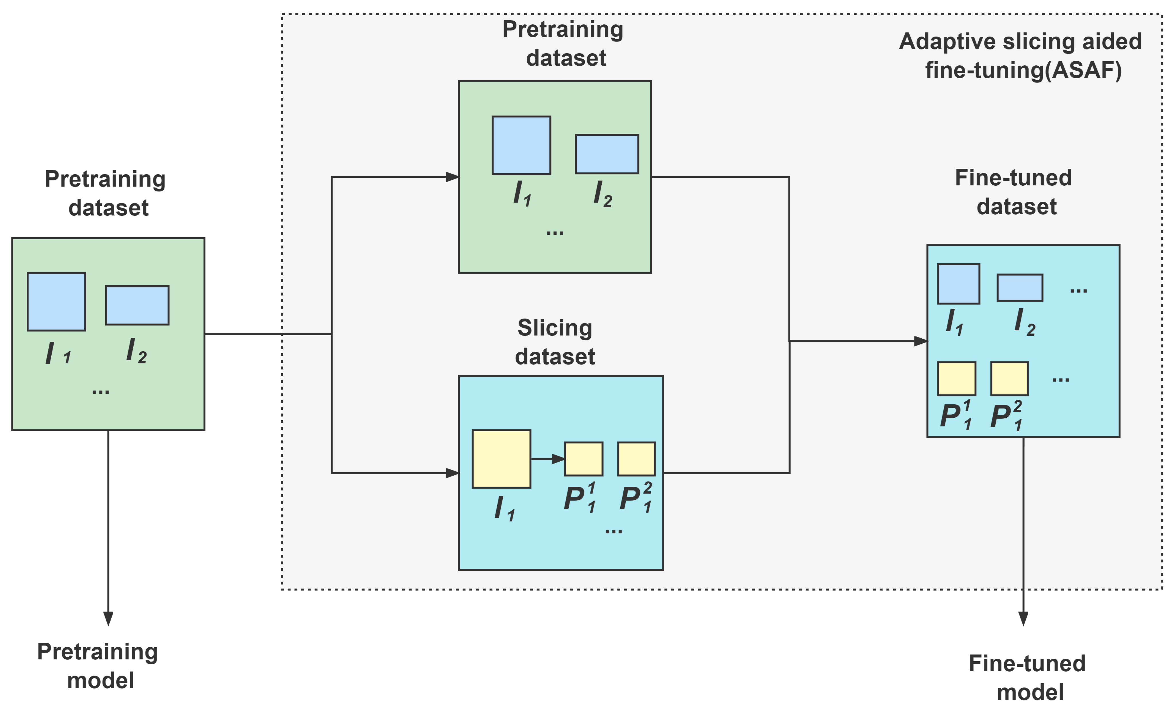
3.4. Adaptive Slicing-Aided Fine Tuning

In ASAF, the widely used TPH-YOLOv5 object detection framework [10] provides pre-trained weights on datasets such as VisDrone. This allows the model to be fine-tuned using smaller datasets with shorter training times, rather than training from scratch with large datasets. These pre-trained models provide successful detection performance for similar inputs. In ASAF, as shown in Figure 7, $I_1,I_2,\dots ,I_j$ are sliced into overlapping patches $P_1,P_2,\dots ,P_j$ by ASAHI to form the sliced dataset. Together with the original pre-trained dataset, we set up our complete fine-tuned dataset. Considering the large number of images after slicing, which imposes a large burden on the training process, we have not used other data augmentation techniques such as rotation, geometric distortions, or photometric distortions.

4. Experiments

4.1. Datasets and Settings

We used two datasets, VisDrone2019 and xView [19], to evaluate our model, and we report our results using the metrics of mAP50 (the average of all ten IoU thresholds with a range of 0.5), mAP50_s ($\mathrm{area}<{32}^2$), mAP50_m (${32}^2\le \mathrm{area}\le {96}^2$), and mAP50_l ($\mathrm{area}>{96}^2$). Here, the VisDrone2019-DET dataset is the same as the VisDrone2021-DET dataset and the VisDrone2022-DET dataset.

VisDrone2019-DET [18] is an object detection dataset consisting of 8599 UAV aerial images taken at different locations and altitudes. It includes 6471 images in the training set, 1580 in the test set, and 548 in the validation set. Most of the images in this dataset have the following characteristics: (1) objects occupying small areas are densely distributed, (2) certain objects are obscured, and (3) reflections, photometric shifts, viewpoint shifts, and similar phenomena are present. The bounding boxes of more than 540,000 objects are annotated using ten predefined categories: pedestrian, person, bicycle, car, van, truck, tricycle, awning-tricycle, bus, and motor.

xView [19] is a large dataset for object detection from remote sensing images. It contains a large number of remote sensing images taken around the world, all of which have high resolutions, i.e., $3093\times 2931$. xView [19] includes more than one million object instances from 60 different categories. During the experiment, we randomly selected 90% and 10% of the images to form the training and validation sets, respectively.

4.2. Implementation Details

The training and testing of our model used a single NVIDIA RTX3080 GPU, and others were tested on a single NVIDIA RTX2080 Ti GPU. In the training phase, we used a pre-trained TPH-YOLOv5 model [10] with dataset fine-tuning for training and evaluation of the ASAHI algorithm. After using ASAF, the training set of the fine-tuning dataset contained 50,708 slicing images and 6471 original images. The sliced images were smaller than the original images. Next, we set the long side of the images to 416 pixels and the batch size to 32. We trained the model for 120 epochs, with the first two epochs used for warm-up. The Adam optimizer was used in the training process, and we used $3\times {10}^{-3}$ as our initial learning rate, with the last epoch decaying to 0.12 of the initial learning rate. During inference, the overlapping was set to 0.15, the Cluster-DIoU-NMS matching threshold to 0.5, and the LS to 1818.

4.3. Ablation Studies

VisDrone2019-DET-test is a challenging dataset, containing dark scenes, multi-view shots, and varying resolutions. We illustrated the universality of our slicing method through validation on the test dataset, as detailed in

Table 2. Results of testing the proposed ASAHI method with different slice sizes and the baseline SAHI method with a fixed slice size of 512 on the VisDrone2019-DET-test dataset. The best results are indicated in bold.

Set Up	img/s	mAP50	mAP50_s	mAP50_m	mAP50_l
TPH + ASAHI (4 slice)	5.19	38.7	24.9	56.5	68.8
TPH + ASAHI (6 slice)	4.98	41.6	28.8	58.5	65.3
TPH + ASAHI (12 slice)	2.98	41.9	30.5	56.4	64.3
TPH + ASAHI (15 slice)	2.39	40.9	29.9	55.1	62.9
TPH + SAHI (512) (baseline)	3.69	42.2	29.8	58.5	65.6
TPH + ASAHI (Adaptive)	4.88 (↑1.19)	45.6 (↑3.4)	33.8 (↑4.0)	59.7 (↑1.2)	60.7

. Considering the aspect ratio of the image, we tested several numbers of slices; maintaining the number of slices at 12 achieved the highest mAP50 result. However, 12 slices led to a higher computation time than a smaller number of slices. In SAHI [15], the slicing size is fixed to 512. While this results in a better performance than other sizes, a fixed slice size inevitably causes various degrees of redundant computation problems when using images with different resolutions. As shown in Table 2, we experimented with slices having a fixed size of 512 as well as fixed numbers of 4, 6, 12, and 15 slices, and found that our TPH+ASAHI (Adaptive) slicing method obtained the highest mAP50 score (45.6) and a fast inference speed (4.88), with 6 slices achieving faster computation and 12 slices showing better accuracy. In order to keep 6 and 12 patches, we set the LS (discussed in Section 3.2) to constrain the slicing number based on the image resolution. The mAP performance of ASAHI, with the specific impact of each component, is provided in

Table 3. The importance of each proposed component validated on VisDrone2019-DET-val. Here, PO and CDN stand for overlapping patches and Cluster-DIoU-NMS, respectively. The best results are indicated in bold.

Model	mAP50	mAP50_s	mAP50_m	mAP50_l
TPH + FI	34.2	21.4	53.3	74.4
TPH + ASAHI	54.4	46.6	66.1	58.9
TPH + ASAHI + FI	55.5	46.7	68.1	76.5
TPH + ASAHI + FI + PO	55.5	46.8	68.6	77.6
TPH + ASAHI + FI + PO + ASAF + CDN	56.8	48.4	68.6	72.9

. The results indicate that the proposed approach leads to improved detection performance for both small and medium objects.

4.4. Comparisons with the State of the Art

We conducted comparison experiments with the current state-of-the-art small object target detection algorithms [11,36,37,38] as well as several classical object detection algorithms [2,34]. The details are shown in

Table 4. Comparison of our method with other state-of-the-art object detection methods on VisDrone2019-DET-val. Certain results are taken from other studies, as indicated. The best results are indicated in bold.

Model	mAP	mAP50	img/s
Fast-RCNN [2]	-	38.5	-
Cascade R-CNN + NWD [34]	-	40.3	-
DMNet [39]	28.2	49.3	-
YOLO-UAV [40]	30.5	-	-
HIT-UAV [38]	-	55.8	-
CRENet	33.7	54.3	1.10
GLSAN [36]	30.7	55.4	-
QueryDet [11]	33.9	56.1	2.75
ClusDet [37]	32.4	56.2	1.29
Focus-And-Detect [33]	42.0	66.1	0.73
TPH + SAHI	34.9	55.1	5.01
TPH + ASAHI(ours)	35.4	56.8	4.88

. Our method reached a mAP result of 35.4 and mAP50 of 56.8. Moreover, the corresponding image processing times per second (img/s) of each components tested on VisDrone2019-DET-test are presented in Figure 8, and the discrepancy between the results and processing times of different post-processing methods, when tested on VisDrone2019-DET-val, are shown in

Table 5. The mAP and time consumption results obtained with different post-processing methods under ASAHI on VisDrone2019-DET-val. The best results are indicated in bold.

Model	mAP50	mAP50_s	mAP50_m	mAP50_l	img/s
NMS	55.8	47.4	68.3	72.9	3.06
SOFT-NMS [12]	52.6	44.3	65.8	70.0	2.72
WBF [13]	55.1	46.7	67.5	73.3	2.88
Cluster-GIoU-NMS	56.3	48.0	68.5	72.9	5.17
Cluster-CIoU-NMS	56.8	48.4	68.6	72.9	4.87
Cluster-DIoU-NMS [35]	56.8	48.4	68.6	72.9	5.26

. CDN obtained the highest mAP50 result of 48.4 and 68.6 for small and medium objects, and maintained the fastest detection speed of 5.25. The comparisons of each proposed component combined with SAHI [15] and ASAHI validated on the VisDrone2019-DET-val dataset are shown in

Table 6. The importance of each component as validated on VisDrone2019-DET-val. The best results are indicated in bold.

Model	mAP50	mAP50_s	mAP50_m	mAP50_l
TPH + FI	34.2	21.4	53.3	74.4
TPH + SAHI	54.2	45.7	66.8	69.0
TPH + SAHI + PO	54.8	46.2	67.8	67.2
TPH + SAHI + FI	54.6	45.7	68.3	75.2
TPH + SAHI + FI + PO	55.1	46.1	68.8	74.6
TPH + SAHI + FI + PO + ASAF + CDN	56.5	48.1	69.0	72.7
TPH + ASAHI	54.4	46.6	66.1	58.9
TPH + ASAHI + FI	55.5	46.7	68.1	76.5
TPH + ASAHI + FI + PO	55.5	46.8	68.6	77.6
TPH + ASAHI + FI + PO + ASAF + CDN	56.8	48.4	68.6	72.9

. ASAHI performed very well on each component, especially detecting small objects, for which it obtained an mAP50 result of 56.8 and an mAP50_s result of 48.4.

5. Results and Limitations

Overall, ASAHI achieved good performance and fast inference speed on both the VisDrone2019-DET [18] and xView [19] datasets. It is worth noting that the performance on xView [19] was outstanding; this is notable because the resolution of most images in the xView [19] dataset is large, which causes significant problems for existing feature extraction algorithms. ASAHI can significantly improve this situation thanks to the proposed adaptive slicing method.

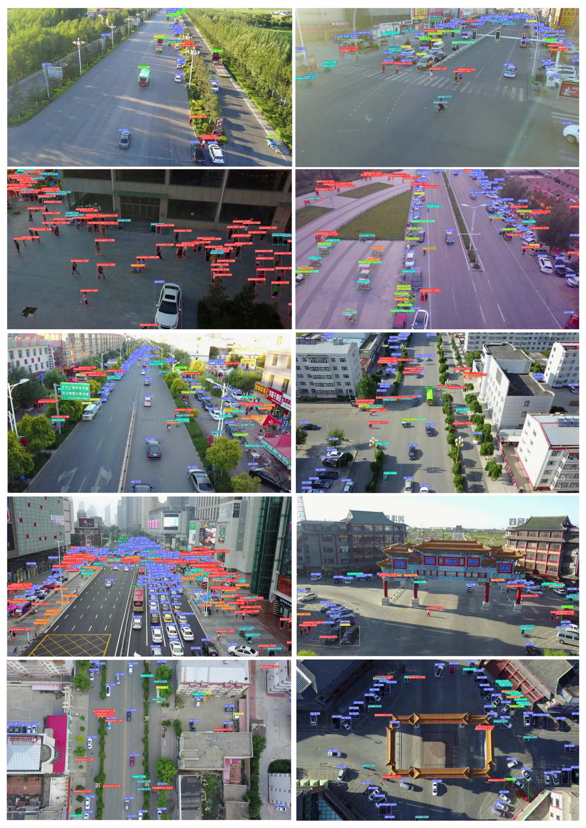
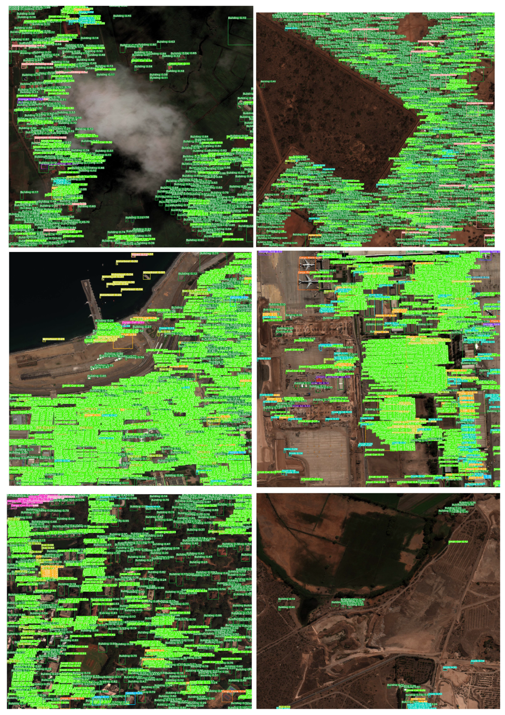
In Figure 9 and Figure 10, we exhibit a portion of the detection results of ASAHI on VisDrone and xView for small objects. As can be seen in Figure 9, ASAHI performs well in various challenging scenes, such as dark scenes (as shown in the third example), scenes with reflections and different shooting angles, and scenes with high density (as shown in the seventh example). Moreover, as shown in Figure 10, ASAHI performs equally well on remote sensing scenes, such as those with extremely large image resolutions, numerous interference factors (as shown in the first example), and multiple detection categories (as shown in the fourth example).

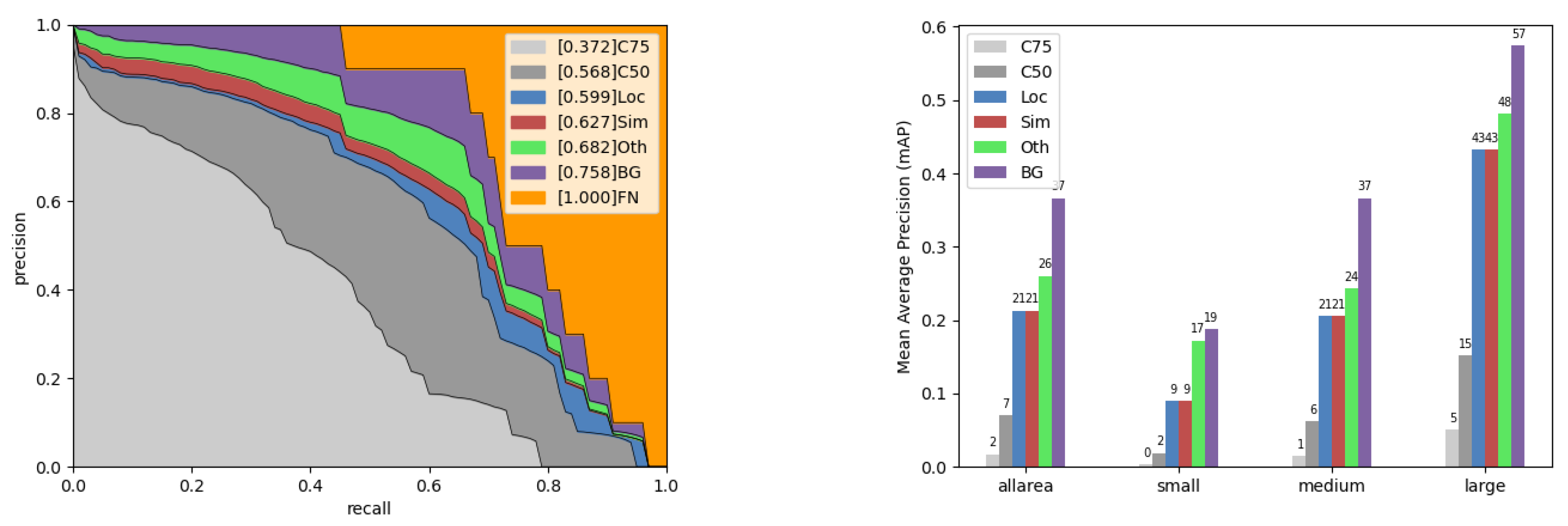
However, this approach has two notable shortcomings: (1) improving the detection accuracy for small objects inevitably leads to a reduction in the detection accuracy for large objects, and (2) a number of error cases remain, such as location and category confusion. The error analysis results of ASAHI on VisDrone and xView are presented on the left and right of Figure 11, respectively. Among these results, C75 (IoU threshold of 0.75), C50 (IoU threshold of 0.5), Loc (ignore location error), Sim (ignore super-category false positives), Oth (ignore category confusions), BG (ignore all false positives), and FN (ignore all false negatives) in Figure 11 clearly show that there is room to improve the error in terms of super-category false positives, category confusion, false positives, and false negatives.

6. Conclusions

In this study, we addressed the redundant computation problem of the generic SAHI slicing method [15]. We proposed a novel adaptive slicing framework, ASAHI, which slices images into a corresponding number of slices rather than using a fixed slice size. This substantially alleviates the problem of redundant computation. TPH-YOLOv5 [10] was used as the backbone to conduct relevant test experiments on the xView [19] and VisDrone2019 [18] datasets. In the post-processing stage, we replaced the traditional NMS with Cluster-NMS to improve the detection speed. Our model realizes improvements in mAP and reduces the time consumption by about 25% compared to SAHI [15] (baseline). Our method is equally applicable to other YOLO-based models. In future work, we plan to use coordinate attention [41] and CSWin Transformer [42] to improve the sensitivity of the proposed method to small objects.