Quantitative Short-Term Precipitation Model Using Multimodal Data Fusion Based on a Cross-Attention Mechanism

Abstract

Short-term precipitation prediction through abundant observation data (ground observation station data, radar data, etc.) is an essential part of the contemporary meteorological prediction system. However, most current studies only use single-modal data, which leads to some problems, such as poor prediction accuracy and little prediction timeliness. This paper proposes a multimodal data fusion precipitation prediction model integrating station data and radar data. Specifically, our model consists of three parts. Firstly, the radar feature encoder comprises a shallow convolution neural network and a stacked convolutional long short term memory network (ConvLSTM), which is used to extract the spatio-temporal features of radar-echo data. The weather station data feature encoder is composed of a fully connected network and an LSTM, which is used to extract the sequential features of the weather station data. Then, the cross-modal feature encoder obtains cross-modal features by aligning and exchanging the feature information of the radar data and the weather station data through the cross-attention mechanism. Finally, the decoder outputs the quantitative short-term precipitation prediction value. Our model can integrate station and radar data characteristics and improve prediction accuracy and timeliness, and can flexibly add other modal features. We have verified our model on four short-term and impending rainfall datasets in South Eastern China, achieving the best performance among the algorithms.

1. Introduction

Due to the need to provide early warnings and guide the arrangement of production activities in urban commerce, social security, disaster prevention and mitigation, infrastructure construction, and other fields [1], the task of quantitative short-term precipitation prediction has become a major focus of research in recent years. However, due to the intricacy of meteorological analysis, the application of artificial intelligence in weather forecasting is still in its infancy. In recent years, researchers have become increasingly interested in employing artificial intelligence to produce reliable, quantitative forecasts of short-term precipitation.

Short-term precipitation prediction utilizes historical multi-source radar data and measurements of meteorological variables from ground-based weather stations to forecast rainfall over the next several hours. Short-term precipitation prediction research approaches can be classified into two categories: numerical weather prediction (NWP) and data-driven models based on artificial intelligence. After years of development, the NWP approach now plays a crucial role in the long- and short-term forecasting of meteorological systems in several nations. However, the NWP approach struggles to produce accurate forecasts for small-scale weather systems with short generation and extinction periods. With the continued application of various new forms of detection equipment and methods to the field of weather forecasting, the types of detection data have expanded to include all types of meteorological radar and ground meteorological station data. Additionally, their spatio-temporal resolution has also been significantly enhanced, providing data support for the application of artificial intelligence technology. One of these methods is the use of a spatio-temporal sequence prediction model driven by several radar-echo data types. These models predict future radar-echo data and invert precipitation using the potential movement law learned from radar-echo data, such as ConvLSTM [2] and its variants [3,4,5]. However, such models suffer from gradient disappearance and poor long-term forecast accuracy, and the complicated nonlinear connection between precipitation and radar reflectivity creates new inaccuracies in the retrieval of precipitation.

Another type of spatio-temporal prediction model based on data driven by ground-observation stations utilizes meteorological elements, such as temperature, humidity, pressure, and precipitation, to predict impending rainfall. Machine-learning methods include random forest [6], the autoregressive integrated moving average model (ARIMA) [7], k-nearest neighbor (KNN) [6], and other machine-learning methods [8,9,10,11]. Deep-learning methods include LSTM [12] and gate recurrent unit (GRU) [13]. These models have made some progress in short-term precipitation prediction based on single-station data. In order to improve these models, a number of researchers have proposed a spatio-temporal graph convolutional neural network (GCN) [14,15,16] for short-term precipitation prediction, where the GCN network is utilized to capture unstructured spatial correlations and an LSTM or GRU is used to capture temporal correlations. Deep neural networks then transfer the collected spatio-temporal data to rainfall values. However, such networks often require an extra input-adjacency matrix and feature a certain temporal latency. Some studies incorporated a radar-echo map into the GCN network to aid in the building of an adjacency matrix in order to determine the spatio-temporal correlation in the precipitation region [17]. The question of how to fully utilize the spatio-temporal properties of radar-echo sequence to examine the dissipation and movement of precipitation clouds has therefore become a core issue in the research on short-term precipitation forecasting. In addition, combining multi-source ground-observation data and radar-echo data to study the geographical distribution of and temporal changes in precipitation during imminent precipitation is a significant challenge.

The most recent advancements in the field of multimodal fusion offer novel solutions for the aforementioned challenges, among which, the cross-modal fusion model based on transformer has been effectively used in Visual Question Answering (VQA), Visual Reasoning in the Real World (GQA), and other fields [18,19,20,21]. This type of model typically consists of multiple encoders, including an object-relation encoder, a language encoder, and a cross-modal encoder. Inspired by this, this paper proposes a new general framework for data fusion between radar-echo maps and ground meteorological station data, called the model based on multimodal data fusion and cross-attention mechanism for precipitation (MFCA). It performs the inductive analysis of the intensity and movement trend of precipitation clouds in the radar-echo map, and combines the past precipitation of the station to realize the short-term and imminent precipitation prediction. Our model overcomes the problems of the time lag and single-data mode in past forms of artificial-intelligence-based, quantitative short-term precipitation and improves prediction accuracy. In the proposed model, we extract the feature vectors of the radar-echo map and the station data at each time step through different encoders and stack the feature vectors at all times in the past as the input of the cross-modal feature encoder. Then, we use the transformer and cross-attention mechanism to model the spatio-temporal rainfall process and predict the future precipitation through the deep neural network. Our main contributions to the forecasting of quantitative short-term precipitation are as follows:

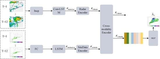
• We propose a new framework called MFCA. MFCA can fuse radar-echo data with station-rainfall data, analyze the spatio-temporal dependence of radar reflectivity and rainfall in the process of rainfall, and predict quantitative short-term precipitation. To our knowledge, we are the first to propose a multimodal-fusion, quantitative short-term precipitation prediction model based on a cross-attention mechanism.
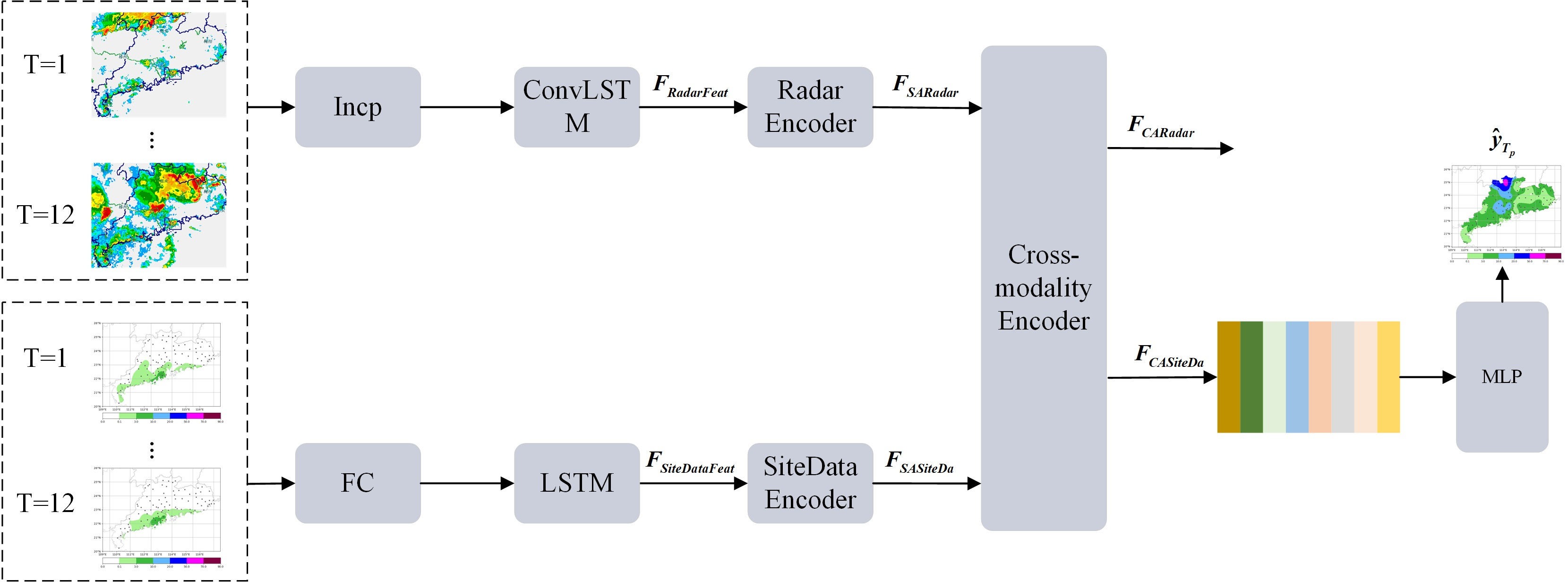
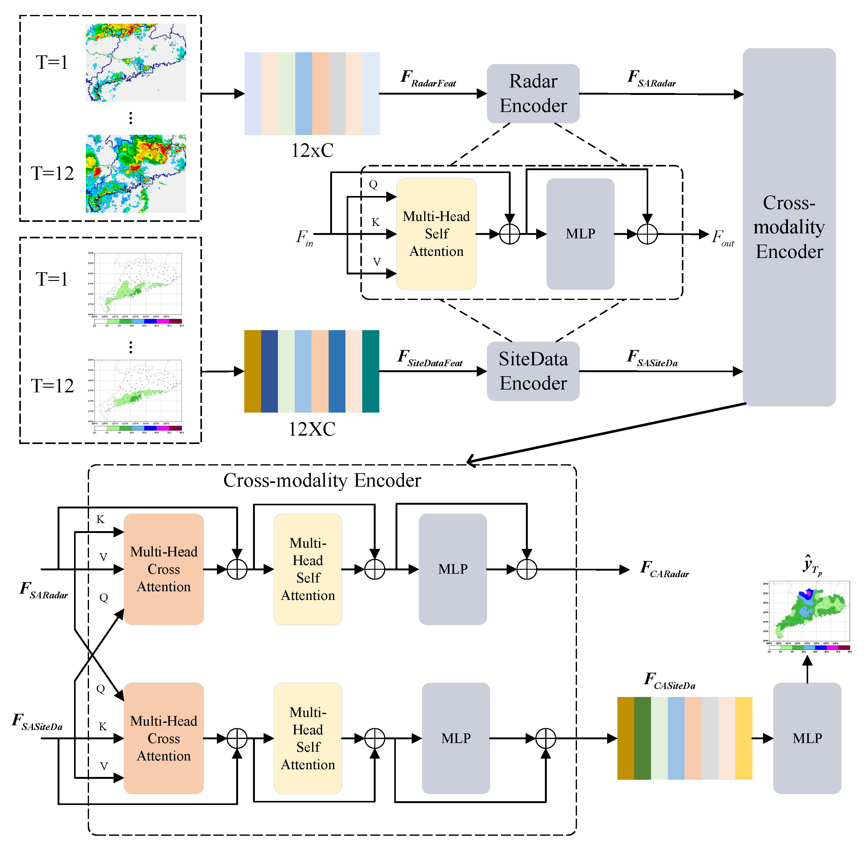
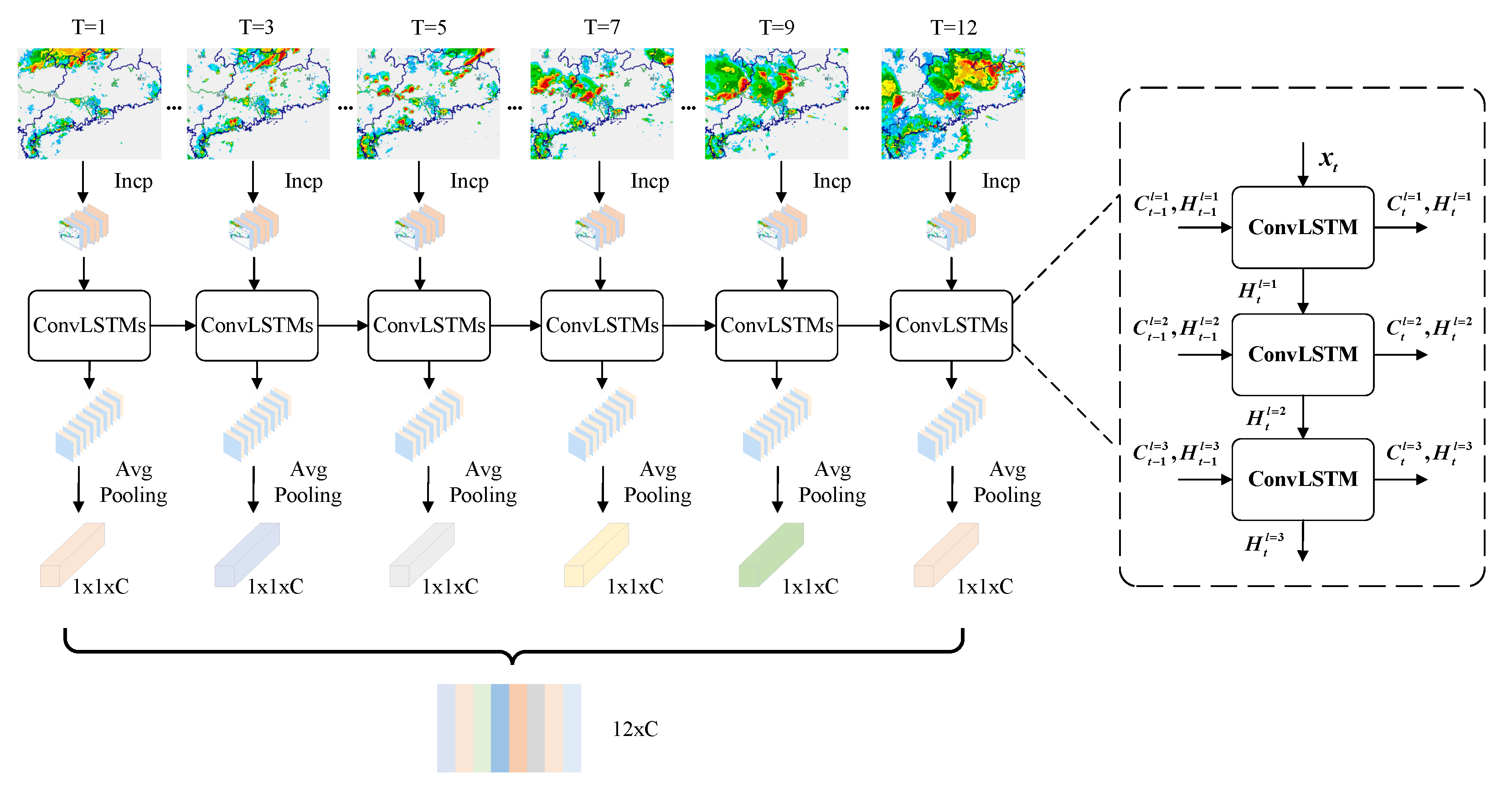
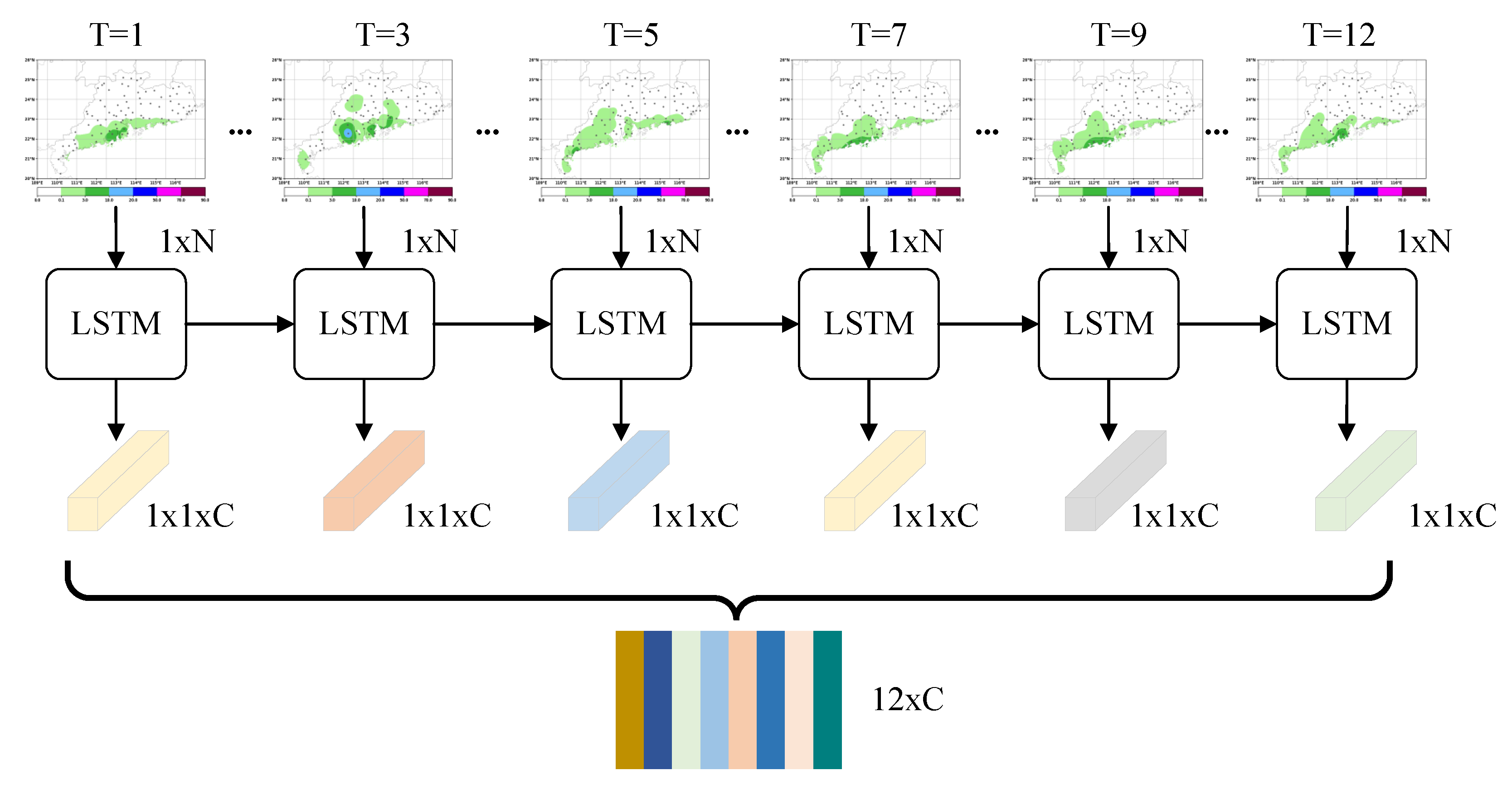
• We present a new feature encoder for radar-echo and station data that uses ConvLSTM, LSTM, and a transformer to extract coded features from different modal weather data. We use the implicit state of each time step as the feature of the time step, and use a transformer to further encode it, and then exchange features through the cross-attention mechanism.
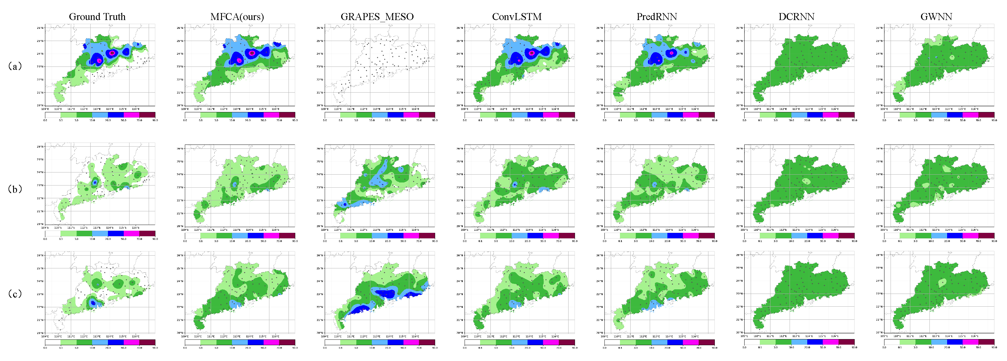
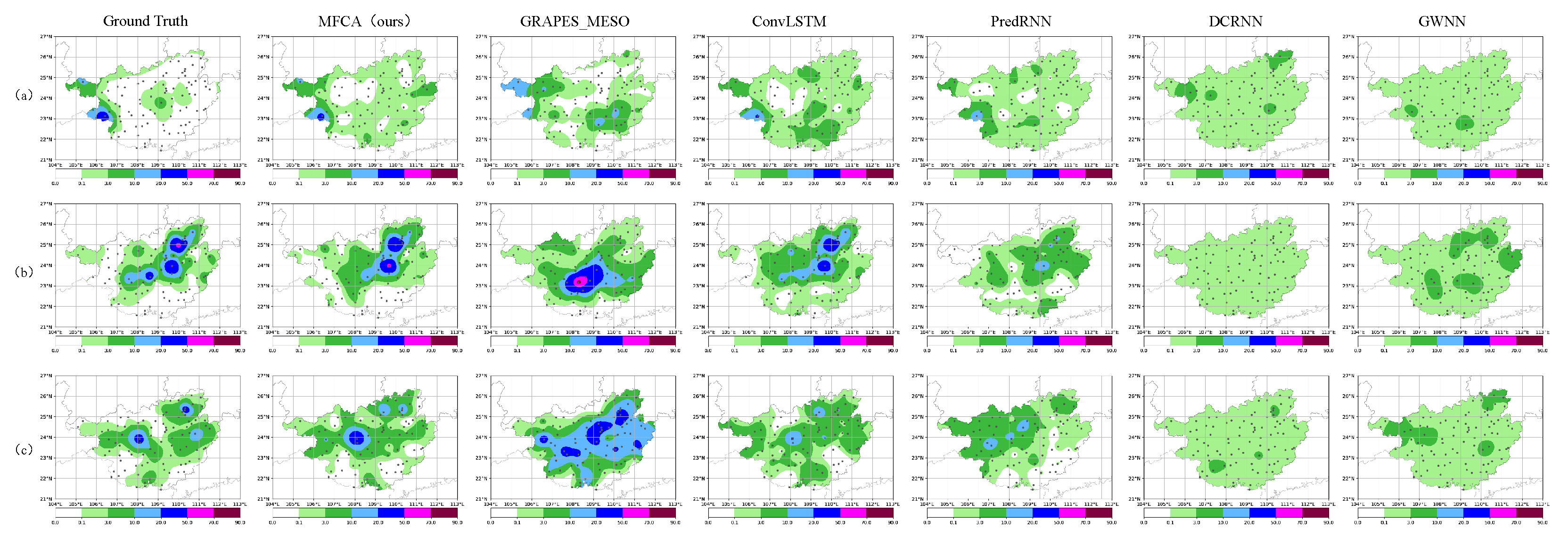
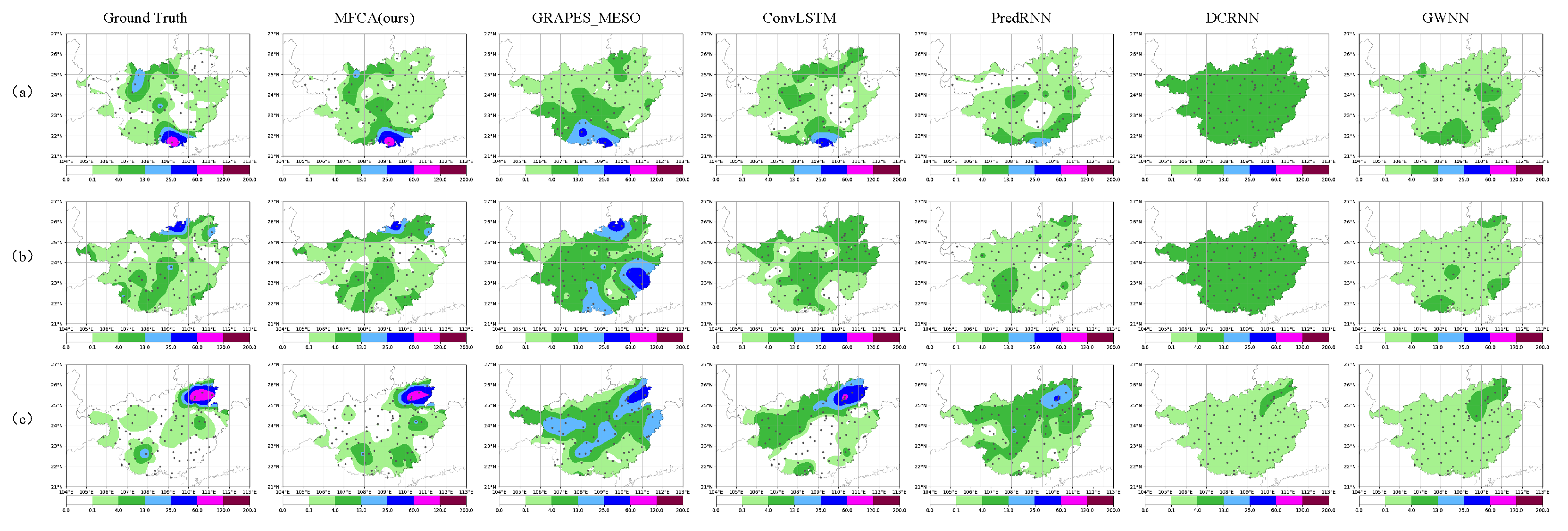
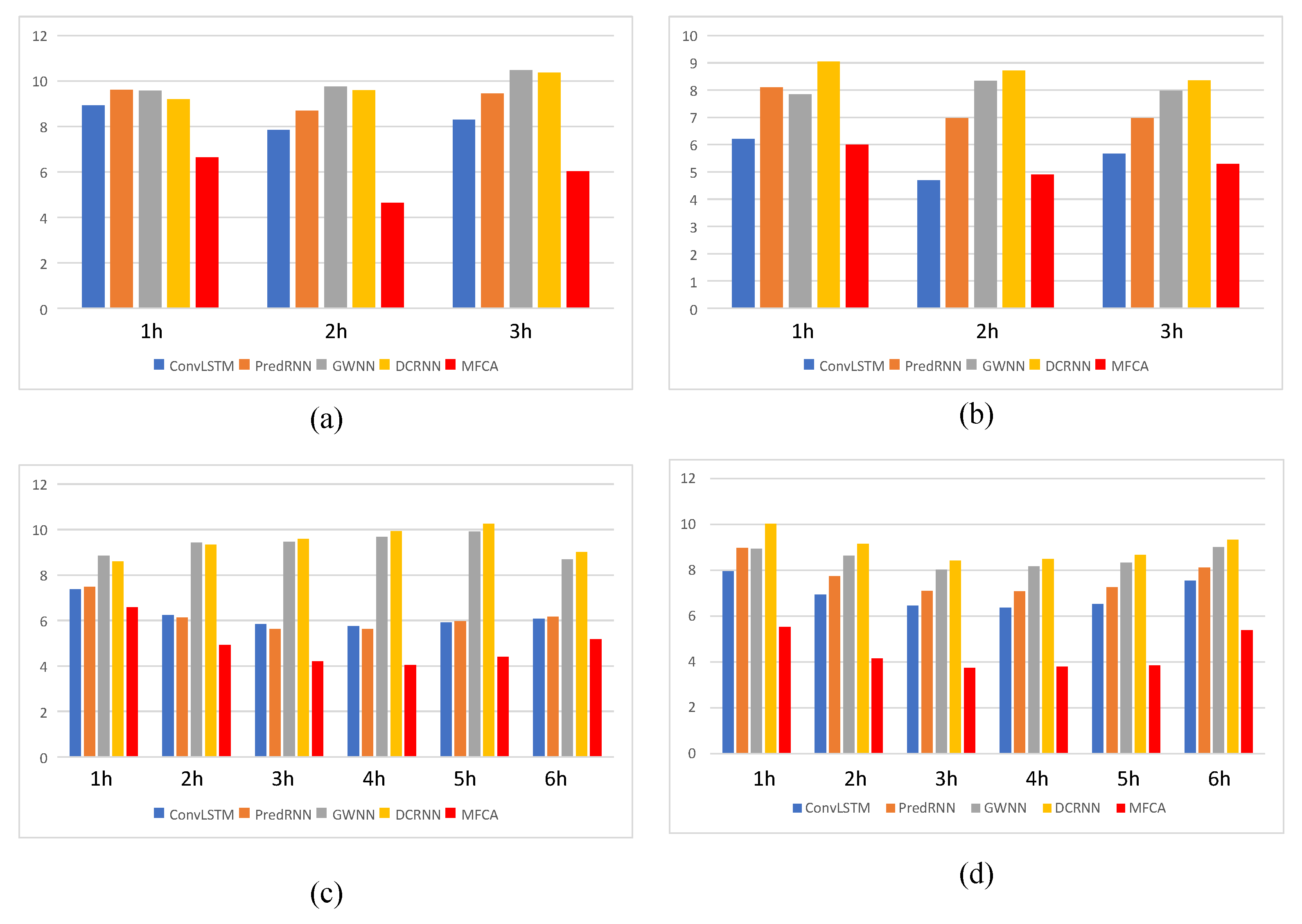
• We validated our model on four real datasets from southeastern China, and compared it with a current, mainstream, advanced, single-mode rainfall prediction model. The results of the experiments confirm the superiority of our model.

2. Related Work

The first section of this chapter introduces the relevant uses of ConvLSTM and LSTM in the prediction of short-term and imminent precipitation. The second section introduces the recent development of a multimodal fusion algorithm based on the transformer architecture. The third section introduces the convection-allowing forecast model (CMA).

2.1. Spatio-Temporal Model

Precipitation prediction is a task of spatio-temporal sequence modeling. The model learns potential change rules from many spatio-temporal sequence data through training. By evaluating a period of historical spatio-temporal data, the trained model can predict the future changes in spatio-temporal data. Numerous studies have investigated this endeavor. Zhang proposed a multi-channel 3D-cube successive convolution network (3D-SCN) [22] to predict the emergence and development of convective storms utilizing multi-source meteorological data. Studies revealed that the prediction accuracy of the model is higher than that of the conventional model. Researchers presented the geospatial-temporal convolutional neural network (GT-CNN) based on a 3D convolution neural network (3D-CNN) and LSTM [23]. In this model, 3D-CNN is used to construct the geospatial relationships between various sampling points. LSTM is used to grab the precipitation features with time information. Shi creatively enhanced LSTM, put forward ConvLSTM [2], and created a spatio-temporal sequences prediction model that could be trained end-to-end. ConvLSTM replaced the full connection procedure in LSTM with convolution; this will establish the temporal relationship of the local spatial features extracted by convolution. After that, Shi proposed Trajectory GRU (TrajGRU) [24], which can actively learn the position changes of objects in spatio-temporal motion, and created an encoder-–forecaster structure. Based on this, researchers proposed a number of spatio-temporal sequence prediction models by designing new modules to improve the accuracy of prediction, such as Predictive RNN (PredRNN) [25], PredRNN++ [26], Memory In Memory (MIM) [27], Self-Attention ConvLSTM (SAConvLSTM) [28], etc. These models learn potential atmospheric motion laws from a large number of data to deduce radar-echo images and predict short-term precipitation through radar images. The nonlinear mapping link between the radar-echo rate and precipitation must also be investigated in models of this sort. However, the development of this sort of method provides a broad concept through which to create multimodal meteorological data encoders.

2.2. Multimodal Fusion Algorithm

Fusion methods can be broadly categorized into three categories based on distinct fusion operations: basic fusion methods based on splicing and linear combinations [29,30]; basic fusion methods based on the attention mechanism [31,32,33]; and basic fusion methods based on bilinear pooling [34]. The fusion method used in this paper belongs to the second type. Researchers from Google put forward the transformer model in [35], which uses the self attention structure to replace the recurrent neural network (RNN) network structure commonly used in natural language processing (NLP). The transformer has achieved good results in many text and sequence tasks. Moreover, the stacked multi-header self attention structure is widely used in the multimodal fusion model. These multimodal fusion models generally include three encoders: a cross-modal encoder, an object–relationship encoder, and a language encoder. The self-attention layer and cross-attention layer form the foundation of the three encoders. The object–relationship encoder and language encoder are single-mode encoders that focus, respectively, on visual and linguistic data. Each single-mode encoder contains a self-attention layer and a feedforward layer. Each cross-mode encoder consists of two self-attention layers, one bidirectional cross-attention layer, and two feedforward layers.

2.3. Convection-Allowing Forecast Model

The advent of convection-allowing models with sufficiently fine horizontal resolution now enables explicit, deep, moist convection, providing more accurate forecasts of high-impact weather. In addition, the rapidly updated NWP system can use the latest weather observations to provide situational awareness for rapidly evolving weather events, which is a key component of short-term (0–48 h) prediction guidance. The design of HRRR initialization is very important for its application in short-term prediction. HRRR system has made progress in using radar reflectivity observation and hybrid ensemble variational data assimilation. The CAM initialized by the assimilation of both radar and conventional observations is adopted in most operational centers. The successful practice of radar reflectivity in CAM systems shows that considering radar reflectivity in short-term and imminent precipitation forecasting will bring more abundant information.

3. Methods

3.1. Problem Description

Our goal is to combine the last 12 h of meterlogical-station data with radar-echo data in an area to predict short-term precipitation. The site data in the region can be represented as $X_t=[x_t^1,\dots ,x_t^2,\dots ,x_t^N]\in {\mathbb{R}}^{1\times N}$, where $x_t^i$ is the precipitation of the station i at time t. $y_t$ represents the actual ground-observation value at the current location, $y_t=[y_t^1,\dots ,y_t^2,\dots ,y_t^N]\in {\mathbb{R}}^{1\times N}$, where N represents the number of ground meteorological stations. The corresponding predicted value is represented by ${\widehat{y}}_t$. The radar-echo data at time t in this area are represented by matrix $R_t\in {\mathbb{R}}^{D_W\times D_H}$, where $D_H$ represents the height and $D_W$ represents the width of the radar-echo data. Therefore, the task of quantitative short-term precipitation can be summarized as learning a function $y_{T_p}=f(X_{T_i},R_{T_i})$, where $T_i$ represents the input time slice length, and $T_p$ represents the predicted time slice length. Next, we optimize the following problems:

$$min\sum _{t=1}^{T_p}\sum _{n=1}^N\left[L\left(y_t^n,{\widehat{y}}_t^n\right)\right]$$

(1)

where L represents ${\ell }_2$ loss function.

3.2. Network Structure

First, the basic operation of this network is described. This network contains single-mode-feature encoders, cross-mode feature encoders, meteorological-station-sequence feature encoders, and radar-echo-sequence feature encoders. Firstly, the radar-echo-sequence feature coder and the meteorological-station-sequence feature coder extract the features of radar-echo data and the meteorological station data at the past time $T_i$. Then, the features are encoded and aligned via the single-mode feature coder and the cross-mode feature coder. Finally, the precipitation data of N stations at the future time $T_p$ are obtained via the multi-layer perceptron (MLP). The network flow chart of MFCA in shown in Figure 1.

3.2.1. Sequence Feature Encoder

The structure of radar-echo-data feature extractor is shown in Figure 2. In the original radar-echo data $R_t$, each pixel value represents the radar reflectivity of the point and reflects the size and density distribution of precipitation particles within the meteorological target. To extract the properties of radar-echo data, we apply the inception structure, as shown in Figure 3, owing to the size of the picture. In inception, we employ three convolution kernels of varying sizes (1 × 1, 3 × 3, and 5 × 5) and a pooling layer, which increases network sparsity, decreases picture size, and decreases computation. In prior studies, ConvLSTM demonstrated its stability and effectiveness in extracting spatio-temporal dependence, which is of great significance for radar-echo data. Therefore, we use a stacked three-layer ConvLSTM, as shown on the right of Figure 2. (∗ represents the convolution operator and ⊙ represents the Hardman product in the following.)

$$x_t=Incp\left(R_t\right)$$

(2)

$$g_t=tanh\left({\mathcal{W}}_{xg}\ast {\mathcal{X}}_t+{\mathcal{W}}_{hg}\ast {\mathcal{H}}_{t-1}^l+b_g\right)$$

(3)

$$i_t=\sigma \left({\mathcal{W}}_{xi}\ast {\mathcal{X}}_t+{\mathcal{W}}_{hi}\ast {\mathcal{H}}_{t-1}^l+b_i\right)$$

(4)

$$f_t=\sigma \left({\mathcal{W}}_{xf}\ast {\mathcal{X}}_t+{\mathcal{W}}_{hf}\ast {\mathcal{H}}_{t-1}^l+b_f\right)$$

(5)

$${\mathcal{C}}_t^l=f_t\odot {\mathcal{C}}_{t-1}^l+i_t\odot g_t$$

(6)

$$o_t=\sigma \left(W_{xo}\ast {\mathcal{X}}_t+W_{ho}\ast {\mathcal{H}}_{t-1}^l+W_{co}\circ {\mathcal{C}}_t^l+b_o\right)$$

(7)

$${\mathcal{H}}_t=o_t\circ tanh\left({\mathcal{C}}_t^l\right)$$

(8)

$$RadarFea{t}_t=AvgPool\left(MLP\left(H_t^3\right)\right)$$

(9)

where $Incp$ indicates the inception drop sampling network, l indicates the number of layers, W indicates convolution kernel, and b indicates bias. We input the hidden state $H_t^3$, the output of the third layer ConvLSTM, into the MLP and the pooling layer. After that, we get the spatio-temporal feature vector of the radar-echo data $RadarFea{t}_t$ at time t.

The structure of site-data feature extractor is shown in Figure 4. The data of the meteorological stations are the real rainfall $y_t$ of Guangdong and Guangxi Province, China. In this network, we use only one meterlogical obsevation element, rainfall, so the data of stations at each time form a vector with the size of 1xN. The meteorological station data encoder is composed of LSTM and a full connection layer. LSTM models the temporal dependency of time-series data using memory cells and a gating mechanism. If input gate $i_t$ is engaged for each new input, its information is stored in the memory cell; if a forgetting gate is activated, the previously stored information $c_{t-1}$ is forgotten, and the most recent unit output is propagated by output gate $o_t$ to the final state $H_t$. $H_t$ outputs the time feature vector of meteorological station data at time t as $SiteDataFea{t}_t$ through a two-layer fully connected network.

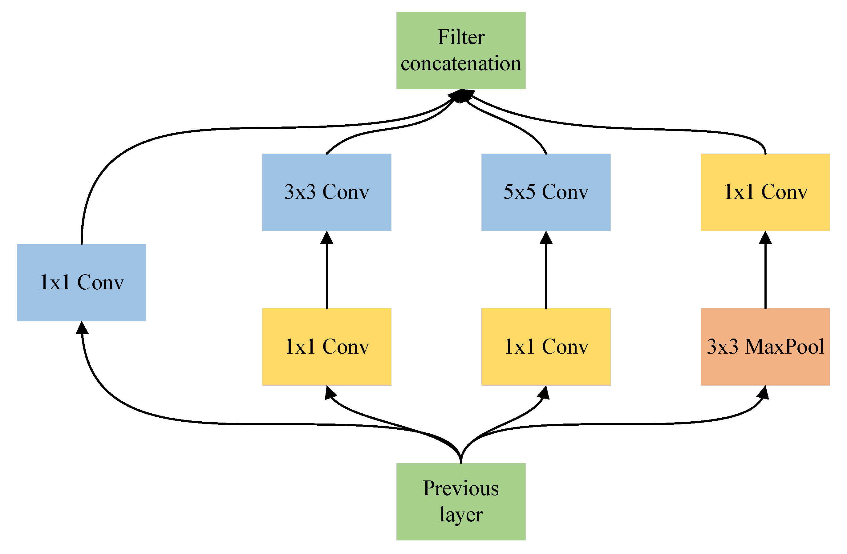
3.2.2. Single-Mode Feature Encoder

Each sub-layer of the single-mode feature encoder consists of a multihead attention sub-layer and a MLP with two fully connected sub-layers. As depicted in the top half of Figure 1, residual connection and normalizing layer were added after each sub-layer to mitigate gradient disappearance and enable faster training. The inputs of the single-mode feature encoder are matrix $F_{RadarFeat}\in {\mathbb{R}}^{T_a\times D_f}$ and $F_{SiteDataFeat}\in {\mathbb{R}}^{T_a\times D_f}$, where $D_f$ is the dimension of feature and $T_a$ is the total length of the input radar-echo data. $F_{RadarFeat}$ and $F_{SiteDataFeat}$ contain the feature vectors of each modal data extracted by the feature extractor at each moment. The outputs of single-mode feature encoder are coding feature $F_{SARadar}\in {\mathbb{R}}^{T_a\times D_f}$ of radar-sequence data and coding feature $F_{SASiteDa}\in {\mathbb{R}}^{T_a\times D_f}$ of site sequence data. In the multi-attentional sub-layer, we calculate the matching between the feature vectors of each moment and the feature vectors of other moments $S{A}_{X\to X}(x_t,\left\{x_0,\dots x_k\right\})$. We multiply eigenvector $x_t$ through three matrices, $W_Q,W_K,$ and $W_V$, and obtain queries $Q_t$, keys $K_t$, and values $V_t$. The point product of $Q_t$ and $K_j$ is used to calculate the similarity score between the feature vector at this time and the feature vector at time j. We divide the score by $\sqrt{d_k}$ and multiply it by $V_j$ through softmax, and add the weighted values of all the features at time ${\alpha }_j{V}_j$ to obtain the new feature vector through the attention-operation mapping of feature vector $x_t$ and matrix $\left\{x_0,\dots ,x_k\right\}$, and the size is the same as $x_t$ after attention operation. The formula is as follows:  

$$a_j=Q_t{K}_j^T/\sqrt{d_k}$$

(10)

$${\alpha }_j=exp\left(a_j\right)/\sum _{k}exp\left(a_k\right)$$

(11)

$$Z_t={\sum }_k{\alpha }_j{V}_j$$

(12)

$$SA=[Z_0,\dots Z_t]$$

(13)

Multi-head attention can be understood as the use of multiple non-interfering self-attention mechanisms, and the outputs of each self-attention mechanism are spliced to obtain multiple outputs $[S{A}_1,\dots S{A}_k]$. The outputs $F_{SARadar}$ and $F_{SASiteDa}$ of the single-mode feature encoder are multiplied by a learnable weight matrix $W_{SA}$. The formula is as follows:

$$F_{SA}=[S{A}_1,\dots S{A}_k]W_{SA}$$

(14)

where $W\in {\mathbb{R}}^{h\times d_k\times d_w}$ and h are the attention mechanisms in multiple attention, and $d_k$ is the dimension count of $K_t$.

In the single-mode feature encoder, we employ a multi-head self-attention mechanism so that feature vectors of radar data and site data can be projected to different representation subspaces via multiple weight matrices. This increases the model’s ability to focus on different features at different times, while maintaining the same size for input and output. Each encoder for a single modal feature concentrates on a single modal feature (radar-echo data or weather-station data).

3.2.3. Cross-Modal Feature Encoder

Each cross-modal layer of the cross-modal feature encoder consists of a bidirectional cross-attention sub-layer $\left(CA\right)$, two self-attention sub-layers $\left(SA\right)$, and two MLPs. Similarly to the single-modal feature encoder, we use a normalization layer and residual connection. Depending on the objective, various numbers of cross-modal layers can be stacked. The output of each layer is the input for the subsequent layer. The bidirectional cross-attention sub-layer consists of two one-way cross-attention sub-layers: radar data to site data $\left(C{A}_{R\to S}\right)$ and site data to radar data $\left(C{A}_{S\to R}\right)$. In layer l, we calculate the similarity between radar-data feature $R_t^{l-1}$ and site-data feature $S_t^{l-1}$ output from layer $l-1$, and output the cross-modal feature of layer L:

$${\widehat{R}}_i^l=C{A}_{R\to S}\left(R_i^{l-1},\left\{S_1^{l-1},\dots ,S_m^{l-1}\right\}\right)$$

(15)

$${\widehat{S}}_j^l=C{A}_{S\to R}\left(S_j^{l-1},\left\{R_1^{l-1},\dots ,R_m^{l-1}\right\}\right)$$

(16)

In order to further establish the internal connections of cross-modal features, we connect a self-attention sub-layer after the cross-modal layer:

$${\tilde{R}}_i^l=S{A}_{R\to R}\left({\widehat{R}}_i^l,\left\{{\widehat{R}}_1^l,\dots ,{\widehat{R}}_n^l\right\}\right)$$

(17)

$${\tilde{S}}_i^l=S{A}_{R\to R}\left({\widehat{S}}_i^l,\left\{{\widehat{S}}_1^l,\dots ,{\widehat{S}}_n^l\right\}\right)$$

(18)

Finally, $\left\{{\tilde{R}}_i^l\right\}$ and $\left\{{\tilde{S}}_i^l\right\}$ output cross modal features $F_{CARadar}=\left\{R_i^l\right\}$ and $F_{CASiteDa}=\left\{S_i^l\right\}$ through the MLP. Our model has two outputs, as shown in the bottom right of Figure 1: feature similar to radar data and another feature similar to site data. As our goal is quantitative short-term precipitation, which is more similar to site data, we use site data as the input to the MLP and decode the linear layer to output the rainfall for the next 3 h or 6 h.

3.3. Implementation

We use the 3 h quantitative short-term precipitation dataset of Guangdong to illustrate the proposed MFCA model. Each batch of training samples consists of a radar-echo data sequence $\left\{R_t\right\}$ with dimensions of 12 × 1 × 280 × 360, where 12 is the number of time steps separated by 1 h, 1 is the number of channels, and 280 × 360 is the size of a single radar images. The size of meteorological-station data series $\left\{X_t\right\}$ is 12 × 1 × 85, where 12 is the time step with an interval of 1h, 85 is the number of meteorological stations, and 1 represents the 1-dimensional real rainfall observation of each station. The size of the training label is 3 × 1 × 85, 3 is the prediction-step size, the interval is 1 h, 1 is the number of channels, and 85 is the number of meteorological stations. First, the radar map sequence was down-sampled through the inception network to obtain a set of feature maps with a size of 12 × 256 × 35 × 45. The 3-layer ConvLSTM network was then inputted in chronological sequence, and the output $H_t^3$ of the third layer for each time step was taken as the temporal and spatial characteristics of the 512 × 35 × 45 radar-echo data. After stacking the characteristics of twelve time steps, the dimensions were 12 × 512 × 35 × 45. Next, we input the MLP and pooling layer to produce the 12 × 1024 dimensional space-time feature vector $F_{RadarFeat}$ of radar-echo data. Simultaneously, meteorological-station data were fed into the LSTM network based on the time step, and time-feature vector $F_{SiteDataFeat}$ of meteorological-station data was produced via two complete connection layers with a size of 12 × 1024.

Next, we input $F_{RadarFeat}$ and $F_{SiteDataFeat}$ into the single-mode feature encoder to enhance semantic feature representation, and then input the output of the single-mode feature encoder into the cross-mode encoder to align and exchange different modal-feature information. The input and output dimensions of these two modules are identical: 12 × 1024. The station-data characteristics provided by the cross-mode encoder were fed into the multilayer perceptron network and the complete connection layer to produce the projected values, with a size of 3 × 85, in order to acquire the expected rainfall values of 85 stations in the next 3 h expressed by $\left\{{\widehat{y}}_{T_p}\right\}$. The algorithmic flow of MFCA is shown in Algorithm 1.

Algorithm 1: Algorithmic flow of MFCA.

Input:$\left\{R_t\right\}$,$\left\{X_t\right\}$ Output:$\left\{{\widehat{y}}_{T_p}\right\}$ 1: for$t<T$ (T is the total number of input frames) do 2:       Inputting $\left\{R_t\right\}$,$\left\{X_t\right\}$ into the sequence feature encoder and output $F_{RadarFeat}$. 3:       Inputting $\left\{{\widehat{y}}_{T_p}\right\}$ into the sequence feature encoder and output $F_{SiteDataFeat}$. 4: end for 5: Inputting $F_{RadarFeat}$, $F_{SiteDataFeat}$ into the single-mode feature encoder and output $F_{SARadar}$, $F_{SASiteDa}$. 6: Input $F_{SARadar}$ and $F_{SASiteDa}$ to the cross modal feature encoder and output $F_{CARadar}$,$F_{CASiteDa}$. 7: Input $F_{CASiteDa}$ to the multilayer perceptron network and output $\left\{{\widehat{y}}_{T_p}\right\}$. 8: return$\left\{{\widehat{y}}_{T_p}\right\}$

4. Data and Experimental Configuration

To evaluate the effectiveness of the MFCA network in predicting short-term precipitation, we separated the radar data and meteorological-station data of Guangdong and Guangxi provinces from June to September between 2016 and 2019 into four datasets. We compared the quantitative precipitation prediction of the future 3 h and 6 h between MFCA and the current mainstream spatio-temporal sequence prediction model on the real datasets of Guangdong Province and Guangxi Province. In this section, we begin by outlining the data’s origin and format, and segmentation of the training set and test set. After that, we introduce the comparison models. Finally, we introduce the experiment’s evaluation criteria.

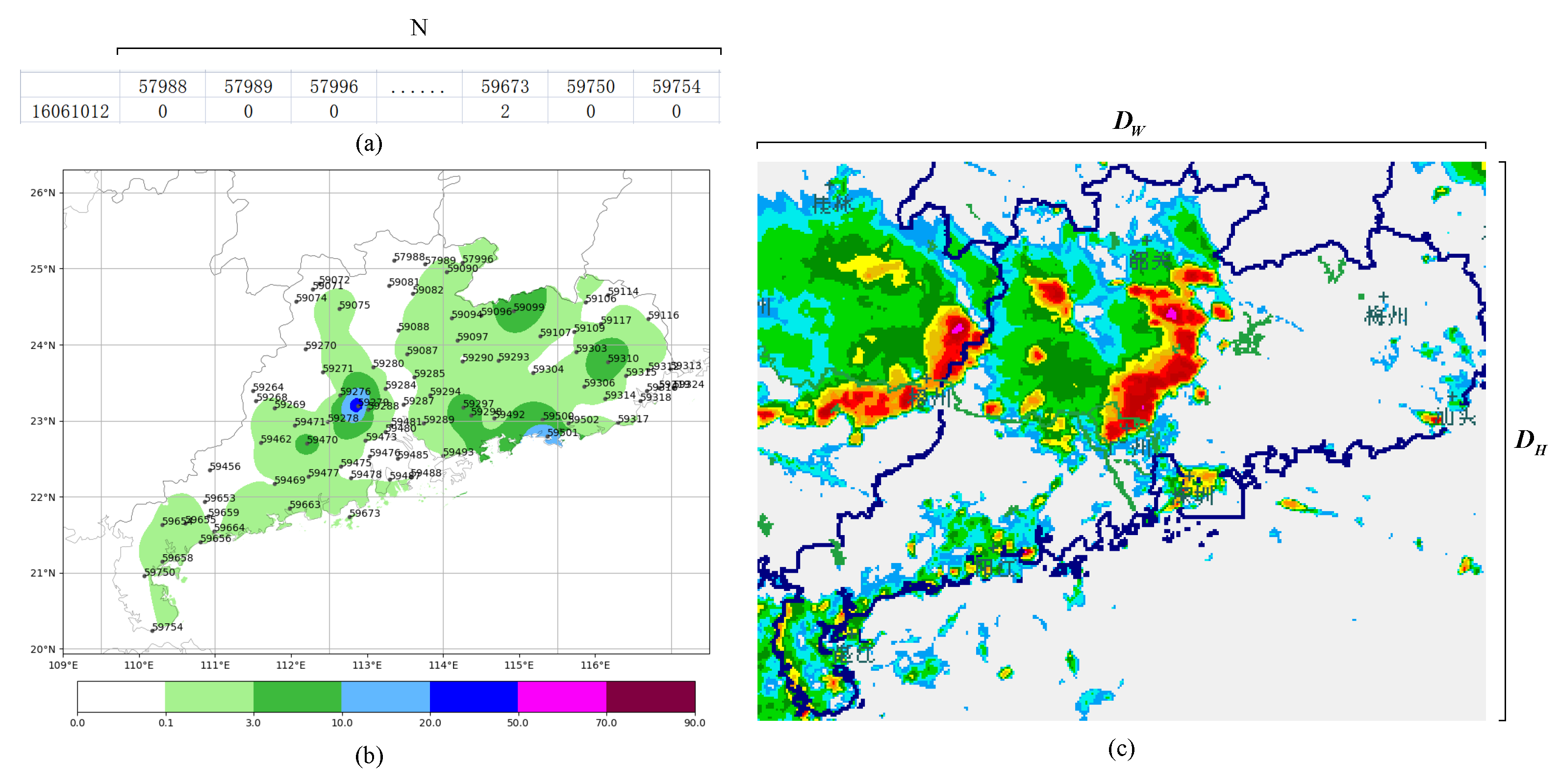
4.1. Data Description and Pretreatment

The original meteorological station data were obtained from National Automatic Station numerical files (http://data.cma.cn/, accessed on 14 April 2022). According to the Chinese automatic station-numbering system, we first checked all the station numbers in the provinces of Guangdong and Guangxi. Next, we extracted the column of hourly precipitation data from each station and stored it as a table according to the station number and time. After cleaning up the retrieved hourly precipitation data, we discovered that certain precipitation data were missing. As our research focused on the continuous rainfall process, we interpolated the missing data based on the station’s previous and subsequent data by linear interpolation. In view of the current requirements for weather forecasting, the 1 h accumulated precipitation is of more practical value. We picked the hourly precipitation of all automated stations in Guangdong Province (as shown on the left of Figure 5) Guangxi Province from June to September 2016 to 2019 as the original meteorological station dataset. The numbers of meteorological stations in Guangdong and Guangxi are 85 and 90, respectively. The meteorological station data interval is one hour, and the data sizes are 11,712 × 85 and 11,712 × 90, respectively. In order to pay more attention to the rainfall process, we used the sliding window to intercept the samples containing the precipitation process. We selected the sample with the average number of precipitation stations at each time of more than 15% of the total. We believe that precipitation was present in this sample. The initial radar mosaic data were 6 min interval radar mosaic data from southeastern China. We cropped the radar mosaic above China’s Guangdong and Guangxi provinces with sizes of 280 × 360 and 263 × 355, as shown on the right of Figure 5, according to the sample time in the selected meteorological station samples. The cropped radar mosaics cover Guangdong or Guangxi and include all the meteorological stations in the provinces of Guangdong and Guangxi. Due to the tiny number of samples missing from the radar map, we decided to exclude the samples missing from the radar map. We obtained the datasets for the multimodal 3 h quantitative short-term precipitation prediction for Guangdong and Guangxi, including 2735 and 2453 groups of samples, respectively. Similarly, we made the datasets for the multimodal 6 h quantitative short-term precipitation prediction for Guangdong and Guangxi, which comprised 2684 and 2397 sample groups, respectively. In the experiment, eighty percent of the data were used as the training set and the remained twenty percent as the test set. We did not use test sets during model training. We predicted the cumulative hourly precipitation for the next 3 or 6 h using precipitation and radar-echo data from the preceding 12 h.

4.2. Comparing Models and Settings

To analyze the performance of our model, we compared it with a number of models that are frequently used in weather-forecasting activities, including:

DCRNN (ICLR2018) [36]: A GCN network that uses a bidirectional random walk on a graph to model spatial dependence and that deploys GCN and GRU for multi-step prediction in coding-–decoder mode.

GWNN (ICLR2019) [37]: A graph neural network based on wavelet basis. By transforming a Fourier basis into a wavelet basis in SpectralCNN, an efficient feature extraction method is implemented. GWNN can effectively learn localized and sparse feature expression and improve the expression effect and operation efficiency of the network.

ConvLSTM (NIPS2015) [28]: A classical spatio-temporal sequence prediction network, which, by extending the fully connected LSTM, features a convolution structure in both input-to-state and state-to-state transitions. A convolution LSTM (ConvLSTM) was used to establish a short-term precipitation forecast model. Extensive studies have demonstrated that ConvLSTM networks can better capture temporal and spatial correlations.

PredRNN (NIPS2017) [25]: A recursive neural network using a unified memory pool to remember spatial representations and temporal variations. Specifically, the memory state is no longer limited within each LSTM cell. Instead, it can zigzag in two directions: vertically, through stacked RNN layers, and horizontally, through the states of all the RNN layers. The core of the network is a new spatio-temporal LSTM (ST-LSTM), which simultaneously extracts and remembers spatial and temporal representations.

A3T-GCN (ISPRSINTJGEO-INF2021) [38]: The model learning the short-term trend in time series using gated recurrent units and the spatial dependency based on the topology is presented to facilitate traffic forecasting. Additionally, the attention mechanism was included to modify the relevance of various time intervals and compile overall temporal data to enhance prediction precision.

PredRNN-V2 (T-PAMI2022) [39]: A recursive neural network which models the structures of visual dynamics by decoupling a pair of memory cells, operating in nearly independent transition manners, and finally forming unified representations of the complex environment. Concretely, besides the original memory cell of LSTM, this network features a zigzag memory flow that propagates in both bottom–up and top–down directions across all layers, enabling the learned visual dynamics at different levels of RNNs to communicate.

GRAPES_MESO: With a geographical resolution of 10 km and a temporal resolution of 3 h, the GRAPES_MESO model predicts precipitation with good accuracy. The maximum time restriction for a forecast is 72 h. Researchers conducted a series of standard and simulation tests, including the analysis and application of conventional data, and the direct analysis and application of nonconventional data, such as radar and satellite data, to validate the accuracy and efficacy of the graphs system. The system has been operational in national and regional meteorological operation centers and has played a significant role in meteorological operations in practice. The model has certain predictive ability for heavy precipitation and other intense weather processes, especially for products with high spatial and temporal resolution, and it can more accurately explain the presence and evolution of the phenomenon.

In this experiment, DCRNN, GWNN, and A3T-GCN predicted the short-term precipitation using the data from the meteorological stations. ConvLSTM, PredRNN, and PredRNN-V2 predicted the short-term precipitation based on the radar data. The Pytorch framework was used to implement all six models, and the GRAPES_MESO model data were obtained from the China National Meteorological Data Center.

4.3. Evaluation Criteria

For the predicted precipitation value, the mean square error (MSE), mean absolute error (MAE), and threat score (TS) were utilized for the quantitative evaluation. The TS score is the World Meteorological Organization’s grading standard for quantitative-precipitation-prediction accuracy and one of the scales used to quantify the accuracy of rainstorm forecasts. The formula for calculating the TS 0.1 threshold at 0.1 mm/h is as follows:

$$TS0.1=\frac{TP}{TP+FN+FP}$$

(19)

$$MSE=\frac{1}{T_p\ast N}\sum _{t=1}^{T_p}\sum _{n=1}^N{\left(y_t^n-{\widehat{y}}_t^n\right)}^2$$

(20)

$$MAE=\frac{1}{T_p\ast N}\sum _{t=1}^{T_p}\sum _{n=1}^N|y_t^n-{\widehat{y}}_t^n|$$

(21)

TP represents true positive, FN represents false negative, FP represents false positive, and TN represents true negative, as shown in

Table 1. Confusion matrix of TS.

		Ground Truth (GT)
		Positive (GT ≥ 0.1)	Negative (GT < 0.1)
Prediction (PD)	Positive (PD ≥ 0.1)	TP	FP
	Negative (PD < 0.1)	FN	TN

.

5. Experimental Results and Analysis

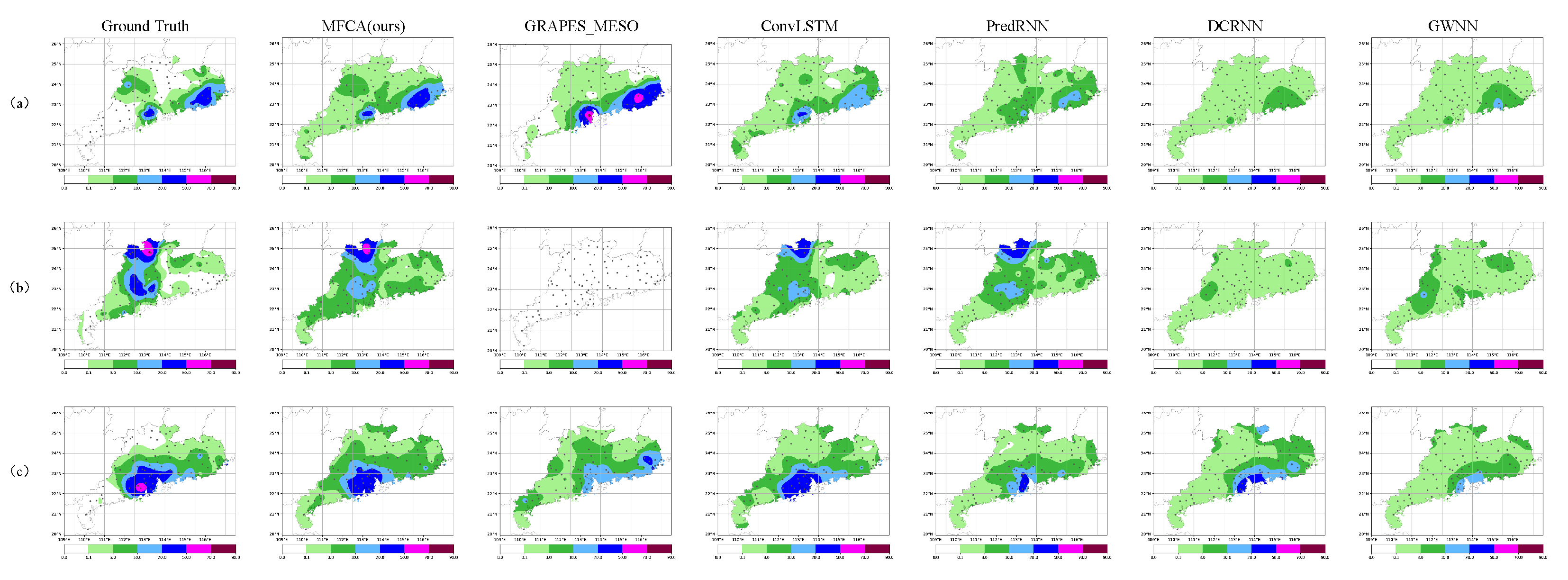
5.1. Performance Comparison

Our comparative experimental results are summarized in

Table 2. Quantitative comparison of accumulated precipitation in Guangdong and Guangxi. The optimal (or suboptimal) results are marked in bold (or underlined).

Methods	Guangdong (3 h)							Guangdong (6 h)
	TS0.1	TS3	TS10	TS20	TS50	MSE	MAE	TS0.1	TS3	TS10	TS20	TS50	MSE	MAE
Ours	0.37	0.44	0.62	0.61	0.44	12.1	1.96	0.54	0.48	0.63	0.67	0.59	14.5	2.75
GRAPES_MESO	0.26	0.18	0.14	0.12	0	72	3.43	0.104	0.06	0.04	0.05	0	119	4.82
DCRNN	0.36	0.24	0.10	0.02	0	47.48	2.9	0.53	0.30	0.03	0.01	0	87.38	4.5
GWNN	0.36	0.25	0.09	0	0	47.84	3.3	0.53	0.26	0.05	0.03	0	88.81	4.52
A3T-GCN	0.38	0.22	0	0	0	49.56	3.20	0.54	0.33	0.14	0.02	0	115.23	5.81
ConvLSTM	0.36	0.39	0.52	0.44	0.1	20.96	2.5	0.53	0.40	0.59	0.56	0.48	24.7	3.55
PredRNN	0.37	0.29	0.27	0.12	0	34.04	2.8	0.54	0.39	0.52	0.49	0.3	31.27	3.89
PredRNN-V2	0.38	0.35	0.37	0.29	0.06	26.82	2.7	0.52	0.42	0.52	0.50	0.3	28.22	3.71
	Guangxi (3 h)							Guangxi (6 h)
Ours	0.41	0.52	0.63	0.54	0.53	9.25	1.78	0.55	0.6	0.72	0.71	0.62	14.17	2.38
GRAPES_MESO	0.36	0.23	0.16	0.06	0	51.91	2.88	0.22	0.1	0.08	0.15	0	105.99	4.48
DCRNN	0.34	0.21	0.03	0.01	0	39.38	2.7	0.50	0.27	0.03	0	0	103.11	5.59
GWNN	0.34	0.24	0.04	0.01	0	39.37	3.12	0.50	0.27	0.04	0	0	103.89	5.41
A3T-GCN	0.35	0.21	0.01	0	0	40.71	2.90	0.50	0.29	0.07	0	0	102.16	5.54
ComvLSTM	0.39	0.37	0.51	0.35	0.22	16.37	2.49	0.53	0.47	0.58	0.53	0.42	29.83	3.57
PredRNN	0.37	0.27	0.18	0.06	0.01	32.42	2.87	0.51	0.39	0.39	0.27	0.17	48.26	4.2
PredRNN-V2	0.38	0.32	0.30	0.21	0.09	25.73	2.8	0.51	0.40	0.43	0.35	0.21	39.13	3.889

. In general, the deep learning method was superior to the NWP approach. GRAPES_MESO, with a grid spacing of 10 km, is unable to resolve convective systems. The poor performance of GRAPES_MESO could be caused by the use of coarse resolution in GRAPES_MESO. In addition, the data assimilation may limit its quality of analysis and forecasting. More refined model numerical prediction data of the Grapes Model may improve performance. Since we could not obtain more refined data, we did not compared it. In meteorological prediction, the numerical forecast approach must be analyzed and merged with other models after the fact. In this work, the deep-learning models focused on the summer rainfall in Guangdong and Guangxi. The predictive power of the deep-learning model based on the radar data was superior to that of the model based on the site data, particularly with regard to the forecasting of heavy precipitation. We believe this was due to the fact that the correlation between the larger echo value in the radar-echo data and the heavy precipitation is simpler to identify. The main architectures of our radar-echo-data feature extractor and site data extractor both adopt the most original models in their respective directions. As our experimental results show, after entering the radar-echo data and site data, the effect did not decline because of more input data, but induced better performance. We think this shows that the model has good feature extraction and alignment ability for data of two modes. We can see that in terms of TS0.1 and TS3, our results are not much better than the suboptimal value, but our model shows more significant advantages when predicting greater precipitation. Compared with the suboptimal network, we have added precipitation observation data’s input and integration strategy. The precipitation observation data have a very intuitive response to the heavy rainfall process, which gives the model a more precise judgment of the heavy rainfall process. Our model has a more significant accuracy advantage than single-mode site data because the radar-echo data can well reflect the intensity and area of precipitation. We can see that these single-mode models using site data perform better on TS0.1 and TS3 indicators but produce poor prediction of heavy precipitation. For the heavy precipitation, the station data are clear. However, these single-mode models using site data produced poor scores in forecasting heavy precipitation, as shown in Figure 6 and Figure 7. This is because these single-mode models using site data tend to bias the prediction value to the median to achieve less MSE Loss.

To illustrate the effect of the method more intuitively, we interpolated the site data into grid data and performed a visualization based on the longitude and latitude of the sites, as shown in Figure 6. In example (b) of Figure 6, only our model predicted the heavy rainfall above the visualization map. In example (a) of Figure 6, our model also made accurate predictions for the two heavy rainfall regions on the right side of the visualization map. The examples in Figure 7, Figure 8 and Figure 9 also demonstrate this.

From Table 2, it can be seen that our model was closer to the actual precipitation in terms of precipitation intensity and range, and as the forecast time increased, it outperformed the models based on site data and radar data. In the forecast of the 6 h cumulative rainfall, the DCRNN and GWNN had a greater tendency toward the median value. In order to assess the accuracy of different models’ predictions of the 3 h and 6 h short-term and imminent-precipitation datasets with more precision, we studied the hourly forecast findings further.

Figure 10 depicts the histogram of the MSE errors between the predicted and actual hourly values for five distinct models. In the forecasts of the 3 h and 6 h short-term and impending precipitation, the two models based on the radar data were superior to those based on the station data, and the MFCA model was superior to those based on the radar data. As the output characteristics of all the time steps were used to produce precipitation values after the decoder, recurrent neural networks did not accumulate errors. We found that the majority of the networks produced poor prediction results in the intermediate stage, which represented the difficulty of prediction in the intermediate stage of the precipitation prediction process, and our model demonstrated some superiority in the intermediate stage of the precipitation prediction process. The results indicate that the MFCA model incorporates radar-echo information, alleviates the difficulty of precipitation prediction in the intermediate stage.

5.2. Ablation Experiment

In the preceding trials, the performance of the MFCA in 3 h and 6 h quantitative short-term precipitation prediction tasks was evaluated. In order to demonstrate the efficacy of this strategy in its entirety, we conducted ablation tests based on various module combinations. After that, we examined the major modules by analyzing the impacts of various convolution kernel combinations in the inception of the sequence feature encoding, evaluating the impact of the feature fusion technique, and analyzing the effect of the number of self-attention-layer stacking layers.

Effects of different combinations of inception structures. As shown in

Table 3. Ablation experiment on the modal-characteristic encoder.

Type	Patch Size/Stride	Input Size	Output Size	MSE	MAE
Inceptionx1 MaxPool	As in Figure 3	B × S × 1 × 280 × 360	B × S × 32 × 140 × 180	14.50	2.75
Conv2d	3 × 3/2	B × S × 32 × 140 × 180	B × S × 64 × 70 × 90
Conv2d	3 × 3/1	B × S × 64 × 70 × 90	B × S × 32 × 70 × 90
Conv2d	3 × 3/2	B × S × 32 × 70 × 90	B × S × 32 × 35 × 45
Inceptionx1 MaxPool	As in Figure 3	B × S × 1 × 280 × 360	B × S × 32 × 140 × 180	20	2.91
Inceptionx1 MaxPool	As in Figure 3	B × S × 32 × 140 × 180	B × S × 64 × 70 × 90
Conv2d	3 × 3/2	B × S × 64 × 70 × 90	B × S × 32 × 35 × 45
Conv2d	3 × 3/1	B × S × 32 × 35 × 45	B × S × 32 × 35 × 45
Inceptionx1 MaxPool	As in Figure 3	B × S × 1 × 280 × 360	B × S × 32 × 140 × 180	27	3.1
Inceptionx1 MaxPool	As in Figure 3	B × S × 32 × 140 × 180	B × S × 64 × 70 × 90
Inceptionx1 MaxPool	As in Figure 3	B × S × 64 × 70 × 90	B × S × 32 × 35 × 45
Conv2d	3 × 3/1	B × S × 32 × 35 × 45	B × S × 32 × 35 × 45
Conv2d	3 × 3/2	B × S × 1 × 280 × 360	B × S × 32 × 140 × 180	17.58	2.80
Conv2d	3 × 3/2	B × S × 32 × 140 × 180	B × S × 64 × 70 × 90
Conv2d	3 × 3/1	B × S × 64 × 70 × 90	B × S × 32 × 70 × 90
Conv2d	3 × 3/2	B × S × 32 × 70 × 90	B × S × 32 × 35 × 45

, during the downsampling of the radar-echo data, the inception comprised many layers of standard 3 × 3 convolution. The combination of one layer and three layers of 3 × 3 convolution provided the best effect on the radar-echo-data feature extraction. As the number of inception layers increased, the complexity of the model increased, and the training became increasingly challenging.

The influence of feature fusion strategy. In order to examine the ability of the cross-attention sub-layer to align and exchange information across the modal features, we replaced the cross-attention sub-layer with the features of the two modes directly after the self-attention sub-layer in order to verify the effectiveness of the feature-fusion strategy. The alignment and interchange of the characteristic data between the radar-echo data and the station data had a beneficial effect on the accuracies of the quantitative short-term precipitation prediction forecasts. After deleting the cross-attention sub-layer, as indicated in

Table 4. Ablation experiment on the modal-characteristic encoder.

Radar_Layers	Site_Layers	Cross_Layers	MSE	MAE
1	2	2	18.9	3.08
2	2	2	16.58	3.02
3	2	2	14.50	2.75
4	2	2	17.87	3.17
3	1	1	18.60	3.24
3	3	3	19	3.21
3	2	0	21	3.4

, the MSE index was 6.5% higher than that of the next-best model.

The effect of stacking self-attention layers. To examine the influence of the number of self-attention layers on the single-mode feature encoder, we combined different layers for the two-mode feature encoder. First, we fixed the site-data characteristics: the cross-modal encoder sub-layer number was 2, the test characteristics of the radar encoder sub-layers were 1 to 3, and we determined that the best effect was achieved when the radar encoder sub-layers numbered 3. Therefore, we fixed the radar-encoder layer number to 3 and then adjusted the site-data-encoder and cross-modal-encoder layer tests. Table 4 below displays the findings, showing that the three-layer radar-data feature encoder, the two-layer station-data encoder, and the two-layer cross-mode encoder had the greatest effect.

To sum up, the multimodal feature-fusion model effectively integrated the features of the two modes in the quantitative short-term precipitation prediction task and improved the prediction accuracy.

6. Discussion

Based on the experimental results, it can be seen that ConvLSTM performed better on our dataset than newer networks, such as PredRNN and PredRNN-v2. We think this is because the goal of predrnn series is to predict long-term graphs, so it is more aimed toward improving the performance of dependence. However, in this paper, in order to avoid the new errors introduced by the modeling of the nonlinear relationship between radar reflectivity and precipitation, we used the high-dimensional features extracted in each time step as the input of the prediction network directly, so the advantages of PredRNN cannot be reflected. On the contrary, because of the complexity of the network, the result is not satisfactory.

We found that the MSE values of our model on the four real datasets are better than those of the precipitation prediction model based on a single mode. In the diagram shown in Figure 7, our model is more accurate at predicting the precipitation area. The experimental results show that our model completed the extraction and feature alignment of different modal features in feature extraction and feature fusion. The extracted features can better reflect the precipitation situation in the past 12 h and the high-dimensional features of radar-echo data, which makes it possible to complete the quantitative prediction of short-term precipitation through external neural networks.

The prominent advantage of our model is the prediction of short-term heavy rainfall, so it can provide early warnings for urban flood prevention, power supply companies, and transportation, thereby providing good application value for smart cities. In this study, we only used the precipitation data among the meteorological station data. In future studies, we can consider adding other meteorological elements, such as wind, wind direction, pressure, and temperature. We believe that adding these meteorological elements will improve the prediction of precipitation and precipitation distribution.

7. Conclusions

In conclusion, we presented a multimodal fusion model for short-term precipitation forecasting. The model initially employs an inception framework and a cyclic convolutional neural network to extract spatio-temporal sequence characteristics, and then encodes single-mode sequence information via a self-attention sub-layer. The characteristics of the two modals are then exchanged and aligned through the cross-attention sub-layer in order to learn the joint cross-mode representation, and the self-attention sub-layer is used to construct the internal link. Multilayer perceptron then outputs the short-term precipitation prediction value. Our experiments demonstrated that the model can successfully increase the prediction performance. The multimodal fusion strategy’s efficacy in the short-term heavy-precipitation forecasting task was also demonstrated. Future research will focus on the effect of alternative fusion techniques in short-term precipitation prediction challenges and the addition of other precipitation-related elements (such as wind speed and altitude).

References

1. Shukla, B.P.; Kishtawal, C.M.; Pal, P.K. Satellite-based nowcasting of extreme rainfall events over Western Himalayan region. IEEE J. Sel. Top. Appl. Earth Obs. Remote. Sens. 2017, 10, 1681–1686. [Google Scholar] [CrossRef]
2. Shi, X.; Chen, Z.; Wang, H.; Yeung, D.Y.; Wong, W.k.; Woo, W.c. Convolutional LSTM Network: A machine learning approach for precipitation nowcasting. In Proceedings of the 28th International Conference on Neural Information Processing Systems-Volume 1, Montreal, QC, Canada, 7–12 December 2015; pp. 802–810. [Google Scholar]
3. Chang, Z.; Zhang, X.; Wang, S.; Ma, S.; Ye, Y.; Xinguang, X.; Gao, W. MAU: A Motion-Aware Unit for Video Prediction and Beyond. Adv. Neural Inf. Process. Syst. 2021, 34, 26950–26962. [Google Scholar]
4. Pan, T.; Jiang, Z.; Han, J.; Wen, S.; Men, A.; Wang, H. Taylor saves for later: Disentanglement for video prediction using Taylor representation. Neurocomputing 2022, 472, 166–174. [Google Scholar] [CrossRef]
5. Fu, L.; Zhang, D.; Ye, Q. Recurrent Thrifty Attention Network for Remote Sensing Scene Recognition. IEEE Trans. Geosci. Remote. Sens. 2021, 59, 8257–8268. [Google Scholar] [CrossRef]
6. Kusiak, A.; Wei, X.; Verma, A.P.; Roz, E. Modeling and prediction of rainfall using radar reflectivity data: A data-mining approach. IEEE Trans. Geosci. Remote. Sens. 2012, 51, 2337–2342. [Google Scholar] [CrossRef]
7. Pfeifer, P.E.; Deutrch, S.J. A three-stage iterative procedure for space-time modeling phillip. Technometrics 1980, 22, 35–47. [Google Scholar] [CrossRef]
8. Tang, T.; Jiao, D.; Chen, T.; Gui, G. Medium- and Long-Term Precipitation Forecasting Method Based on Data Augmentation and Machine Learning Algorithms. IEEE J. Sel. Top. Appl. Earth Obs. Remote. Sens. 2022, 15, 1000–1011. [Google Scholar] [CrossRef]
9. Min, M.; Bai, C.; Guo, J.; Sun, F.; Liu, C.; Wang, F.; Xu, H.; Tang, S.; Li, B.; Di, D.; et al. Estimating Summertime Precipitation from Himawari-8 and Global Forecast System Based on Machine Learning. IEEE Trans. Geosci. Remote. Sens. 2019, 57, 2557–2570. [Google Scholar] [CrossRef]
10. Chen, H.; Chandrasekar, V.; Cifelli, R.; Xie, P. A Machine Learning System for Precipitation Estimation Using Satellite and Ground Radar Network Observations. IEEE Trans. Geosci. Remote. Sens. 2020, 58, 982–994. [Google Scholar] [CrossRef]
11. Pan, Z.; Yuan, F.; Yu, W.; Lei, J.; Ling, N.; Kwong, S. RDEN: Residual Distillation Enhanced Network-Guided Lightweight Synthesized View Quality Enhancement for 3D-HEVC. IEEE Trans. Circuits Syst. Video Technol. 2022, 32, 6347–6359. [Google Scholar] [CrossRef]
12. Luo, C.; Li, X.; Ye, Y. PFST-LSTM: A SpatioTemporal LSTM Model With Pseudoflow Prediction for Precipitation Nowcasting. IEEE J. Sel. Top. Appl. Earth Obs. Remote. Sens. 2021, 14, 843–857. [Google Scholar] [CrossRef]
13. Manokij, F.; Sarinnapakorn, K.; Vateekul, P. Forecasting Thailand’s Precipitation with Cascading Model of CNN and GRU. In Proceedings of the 2019 11th International Conference on Information Technology and Electrical Engineering (ICITEE), Pattaya, Thailand, 10–11 October 2019; pp. 1–6. [Google Scholar]
14. Kipf, T.N.; Welling, M. Semi-supervised classification with graph convolutional networks. arXiv 2016, arXiv:1609.02907. [Google Scholar]
15. Velickovic, P.; Cucurull, G.; Casanova, A.; Romero, A.; Lio, P.; Bengio, Y. Graph attention networks. Stat 2017, 1050, 20. [Google Scholar]
16. Hamilton, W.; Ying, Z.; Leskovec, J. Inductive representation learning on large graphs. Adv. Neural Inf. Process. Syst. 2017, 30, 1024–1034. [Google Scholar]
17. Wu, Y.; Yang, X.; Tang, Y.; Zhang, C.; Zhang, G.; Zhang, W. Inductive Spatiotemporal Graph Convolutional Networks for Short-Term Quantitative Precipitation Forecasting. IEEE Trans. Geosci. Remote. Sens. 2022, 60, 1–18. [Google Scholar] [CrossRef]
18. Krishna, R.; Zhu, Y.; Groth, O.; Johnson, J.; Hata, K.; Kravitz, J.; Chen, S.; Kalantidis, Y.; Li, L.J.; Shamma, D.A.; et al. Visual genome: Connecting language and vision using crowdsourced dense image annotations. Int. J. Comput. Vis. 2017, 123, 32–73. [Google Scholar] [CrossRef] [Green Version]
19. Yu, Z.; Cui, Y.; Yu, J.; Tao, D.; Tian, Q. Multimodal unified attention networks for vision-and-language interactions. arXiv 2019, arXiv:1908.04107. [Google Scholar]
20. Devlin, J.; Chang, M.W.; Lee, K.; Toutanova, K. Bert: Pre-training of deep bidirectional transformers for language understanding. arXiv 2018, arXiv:1810.04805. [Google Scholar]
21. Tan, H.; Bansal, M. Lxmert: Learning cross-modality encoder representations from transformers. arXiv 2019, arXiv:1908.07490. [Google Scholar]
22. Zhang, W.; Han, L.; Sun, J.; Guo, H.; Dai, J. Application of Multi-channel 3D-cube Successive Convolution Network for Convective Storm Nowcasting. In Proceedings of the 2019 IEEE International Conference on Big Data (Big Data), Los Angeles, CA, USA, 9–12 December 2019; pp. 1705–1710. [Google Scholar]
23. Lin, C.W.; Yang, S. Geospatial-Temporal Convolutional Neural Network for Video-Based Precipitation Intensity Recognition. In Proceedings of the 2021 IEEE International Conference on Image Processing (ICIP), Anchorage, AK, USA, 19–22 September 2021; pp. 1119–1123. [Google Scholar]
24. Shi, X.; Gao, Z.; Lausen, L.E.; Wang, H.; Yeung, D.Y.; Wong, W.K.; Woo, W.C. Deep Learning for Precipitation Nowcasting: A Benchmark and a New Model. Adv. Neural Inf. Process. Syst. 2017, 30, 5617–5627. [Google Scholar]
25. Wang, Y.; Long, M.; Wang, J.; Gao, Z.; Yu, P.S. PredRNN: Recurrent neural networks for predictive learning using spatiotemporal LSTMs. In Proceedings of the 31st International Conference on Neural Information Processing Systems, Long Beach, CA, USA, 4–9 December 2017; pp. 879–888. [Google Scholar]
26. Wang, Y.; Gao, Z.; Long, M.; Wang, J.; Philip, S.Y. Predrnn++: Towards a resolution of the deep-in-time dilemma in spatiotemporal predictive learning. In Proceedings of the International Conference on Machine Learning, Stockholm, Sweden, 10–15 July 2018; pp. 5123–5132. [Google Scholar]
27. Wang, Y.; Zhang, J.; Zhu, H.; Long, M.; Wang, J.; Yu, P.S. Memory in memory: A predictive neural network for learning higher-order non-stationarity from spatiotemporal dynamics. In Proceedings of the IEEE/CVF Conference on Computer Vision and Pattern Recognition, Long Beach, CA, USA, 15–20 June 2019; pp. 9154–9162. [Google Scholar]
28. Lin, Z.; Li, M.; Zheng, Z.; Cheng, Y.; Yuan, C. Self-attention convlstm for spatiotemporal prediction. In Proceedings of the AAAI Conference on Artificial Intelligence, New York, NY, USA, 7–12 February 2020; Volume 34, pp. 11531–11538. [Google Scholar]
29. Rao, Y.; Ni, J.; Zhao, H. Deep Learning Local Descriptor for Image Splicing Detection and Localization. IEEE Access 2020, 8, 25611–25625. [Google Scholar] [CrossRef]
30. Sun, L.; Fang, Y.; Chen, Y.; Huang, W.; Wu, Z.; Jeon, B. Multi-Structure KELM With Attention Fusion Strategy for Hyperspectral Image Classification. IEEE Trans. Geosci. Remote. Sens. 2022, 60, 1–17. [Google Scholar] [CrossRef]
31. Li, X.; Yin, X.; Li, C.; Zhang, P.; Hu, X.; Zhang, L.; Wang, L.; Hu, H.; Dong, L.; Wei, F.; et al. Oscar: Object-semantics aligned pre-training for vision-language tasks. In Proceedings of the European Conference on Computer Vision, Glasgow, UK, 23–28 August 2020; Springer: Cham, Switzerland, 2020; pp. 121–137. [Google Scholar]
32. Sun, L.; Cheng, S.; Zheng, Y.; Wu, Z.; Zhang, J. SPANet: Successive Pooling Attention Network for Semantic Segmentation of Remote Sensing Images. IEEE J. Sel. Top. Appl. Earth Obs. Remote. Sens. 2022, 15, 4045–4057. [Google Scholar] [CrossRef]
33. Sun, L.; Zhao, G.; Zheng, Y.; Wu, Z. Spectral–Spatial Feature Tokenization Transformer for Hyperspectral Image Classification. IEEE Trans. Geosci. Remote. Sens. 2022, 60, 1–14. [Google Scholar] [CrossRef]
34. Li, X.; Lei, L.; Sun, Y.; Li, M.; Kuang, G. Multimodal Bilinear Fusion Network With Second-Order Attention-Based Channel Selection for Land Cover Classification. IEEE J. Sel. Top. Appl. Earth Obs. Remote. Sens. 2020, 13, 1011–1026. [Google Scholar] [CrossRef]
35. Vaswani, A.; Shazeer, N.; Parmar, N.; Uszkoreit, J.; Jones, L.; Gomez, A.N.; Kaiser, Ł.; Polosukhin, I. Attention is all you need. Adv. Neural Inf. Process. Syst. 2017, 30, 5998–6008. [Google Scholar]
36. Li, Y.; Yu, R.; Shahabi, C.; Liu, Y. Diffusion convolutional recurrent neural network: Data-driven traffic forecasting. arXiv 2017, arXiv:1707.01926. [Google Scholar]
37. Xu, B.; Shen, H.; Cao, Q.; Qiu, Y.; Cheng, X. Graph wavelet neural network. arXiv 2019, arXiv:1904.07785. [Google Scholar]
38. Bai, J.; Zhu, J.; Song, Y.; Zhao, L.; Hou, Z.; Du, R.; Li, H. A3t-gcn: Attention temporal graph convolutional network for traffic forecasting. ISPRS Int. J. Geo-Inf. 2021, 10, 485. [Google Scholar] [CrossRef]
39. Wang, Y.; Wu, H.; Zhang, J.; Gao, Z.; Wang, J.; Yu, P.; Long, M. PredRNN: A Recurrent Neural Network for Spatiotemporal Predictive Learning. IEEE Trans. Pattern Anal. Mach. Intell. 2022. [Google Scholar] [CrossRef]
Figure 1. Flowchart of the proposed MFCA.
Remotesensing 14 05839 g001
Figure 2. Radar-echo-data feature extractor. This figure shows the structure of the radar-echo-data feature extractor in this model, taking the datasets of Guangdong Province as an example. The right side of the figure shows the structure of a 3-layer-stack ConvLSTM, where x t represents the output of I n c p , and H t l and C t l represent the hidden statue of the l-th ConvLSTM at time t. The image in the first line of the figure is a visual image of radar echo. We extract the characteristics of radar-echo data from the past 12 h; only half of the timesteps are shown, and ellipses replace the other half. The practical steps are the same. In the figure, C represents the extracted feature dimension of each timestep. In this experiment, we used C = 1024.
Remotesensing 14 05839 g002
Figure 3. Inception structure diagram.
Remotesensing 14 05839 g003
Figure 4. Site-data feature extractor. The figure shows the structure of the site-data feature extractor in the model, taking the Guangdong dataset as an example. The image in the first line of the figure is the visual image of the precipitation data interpolated to the station. It is a vector with a size of 1XN when used as the input in the experiment. We extracted the characteristics of the precipitation data from the past 12 h. In the figure, we display only half of the timesteps, and the ellipsis replaces the other half. The actual steps are the same. In the figure, C represents the extracted feature dimension of each time step. In this experiment, we use C = 1024, N is the number of meteorological stations.
Remotesensing 14 05839 g004
Figure 5. In figure (a), taking the observation data of Guangdong Province at 12:00 on 10 June 2016 as an example, the style of station data is shown, where N is the number of stations. The number in the first row is the number of stations. The number in the second row is the hourly accumulated rainfall, in millimeters (mm). Figure (b) is the grid point visualization result of (a) by linear interpolation. Figure (c) is the visualization of the radar-echo of Guangdong Province. In the figure, D W and D H represent the pixel size of the image (c).
Remotesensing 14 05839 g005
Figure 6. Three-hour Guangdong site-data visualization: (a) shows the predicted and true values of 3 h accumulated precipitation at 0:00 on 11 June 2019, (b) shows the predicted and true values of 3 h accumulated precipitation at 12:00 on 11 June 2019, and (c) shows the predicted and true values of 3 h accumulated precipitation at 0:00 on 27 August 2017.
Remotesensing 14 05839 g006
Figure 7. Six-hour Guangdong site-data visualization: (a) the predicted and true values of 6 h accumulated precipitation at 12:00 on 6 June 2017, (b) the predicted and true values of 6 h accumulated precipitation at 12:00 on 10 June 2016, and (c) the predicted and true values of 6 h accumulated precipitation at 12:00 on 25 June 2019.
Remotesensing 14 05839 g007
Figure 8. Three-hour Guangxi site data visualization: (a) the predicted and true values of 3 h accumulated precipitation at 12:00 on 13 June 2016, (b) the predicted and true values of 3 h accumulated precipitation at 12:00 on 26 June 2017, and (c) the predicted and true values of 3 h accumulated precipitation at 12:00 on 1 July 2017.
Remotesensing 14 05839 g008
Figure 9. Six-hour Guangxi site data visualization: (a) the predicted value and true values of 6 h accumulated precipitation at 00 on 31 July 2018, (b) the predicted value and true values of 6 h accumulated precipitation at 12:00 on 30 August 2018, and (c) the predicted value and true values of 6 h accumulated precipitation at 12:00 on 7 July 2019.
Remotesensing 14 05839 g009
Figure 10. Hourly forecast MSE histogram. The x-axis of the Figure is the number of hours, and the y-axis is the value of MSE. (a) The MSE of hourly predicted precipitation and true values on the 3 h quantitative short-term precipitation prediction dataset in Guangdong. (b) The MSE of hourly predicted precipitation and true values on the 3 h quantitative short-term precipitation prediction dataset in Guangxi. (c) The MSE of hourly predicted precipitation and true values on the 6 h quantitative short-term precipitation prediction dataset in Guangdong. (d) The MSE of hourly predicted precipitation and true values on the 6 h quantitative short-term precipitation prediction dataset in Guangxi.
Remotesensing 14 05839 g010