

Transferability of Covariates to Predict Soil Organic Carbon in Cropland Soils
 , ,
, ,  , and
, and
Abstract
:1. Introduction
2. Materials and Methods
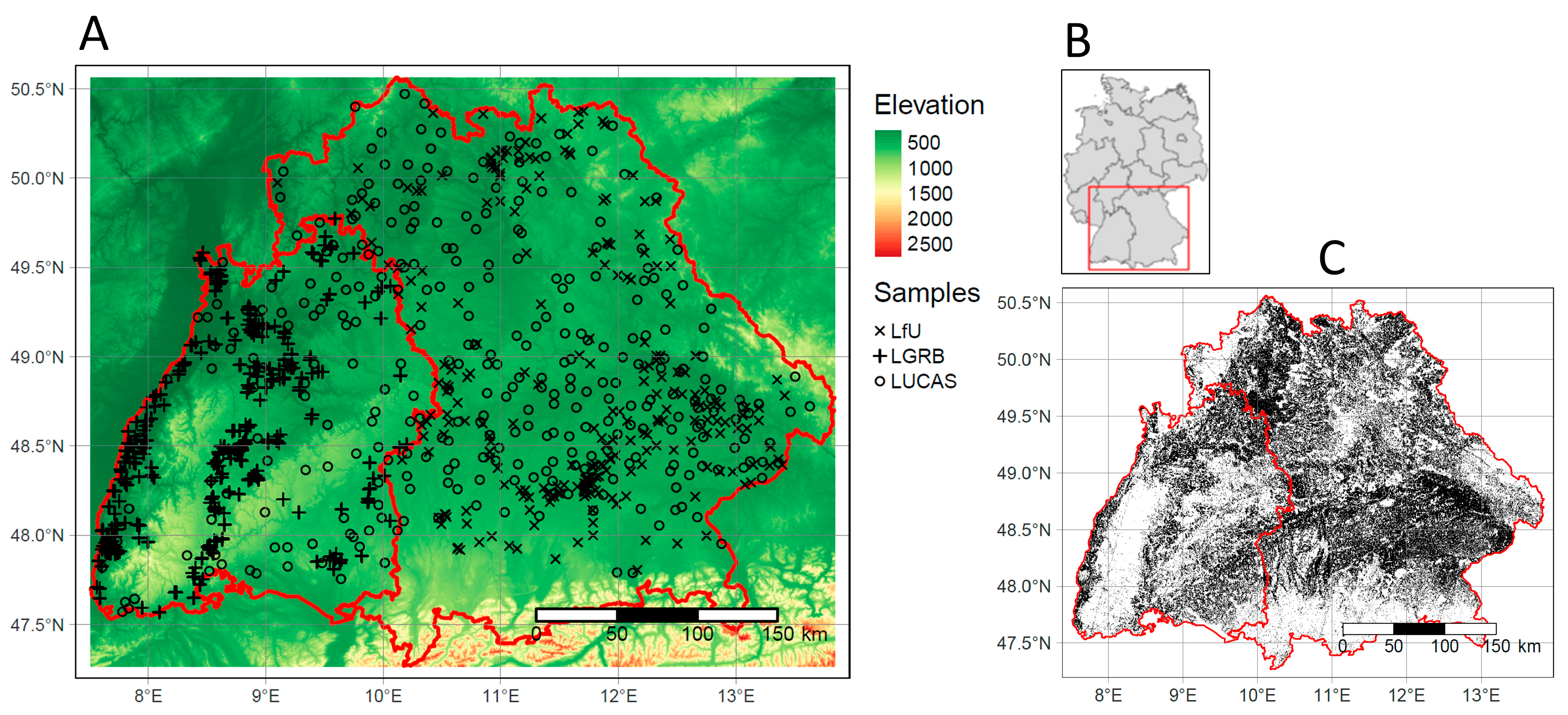
2.1. Study Area
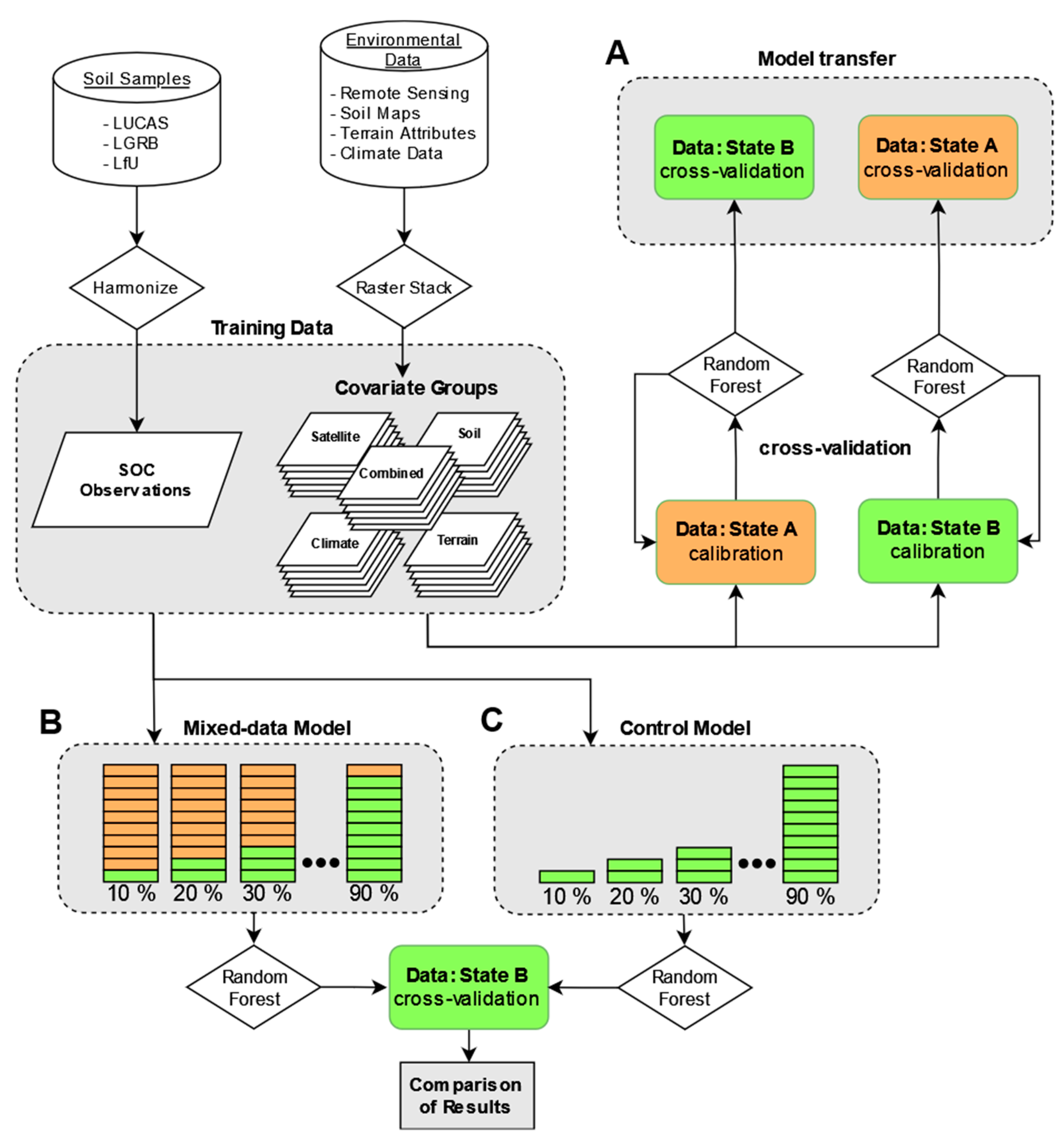
2.2. Procedures
2.3. Soil Samples
2.4. Covariates
2.4.1. Earth Observation
2.4.2. Terrain Attributes
2.4.3. Climate Data

| Group | Covariate | Original Resolution | Layers (n) | Abbreviation | Source |
|---|---|---|---|---|---|
| Satellite | SCMaP Band 1: blue (0.45–0.52 µm) | 30 m | 1 | scmap.1 | [14] |
| SCMaP Band 2: green (0.52–0.60 µm) | 30 m | 1 | scmap.2 | [14] | |
| SCMaP Band 3: red (0.63–0.69 µm) | 30 m | 1 | scmap.3 | [14] | |
| SCMaP Band 4: NIR (0.77–0.90 µm) | 30 m | 1 | scmap.4 | [14] | |
| SCMaP Band 5: SWIR1 (1.55–1.75 µm) | 30 m | 1 | scmap.5 | [14] | |
| SCMaP Band 6: SWIR2 (2.09–2.35 µm) | 30 m | 1 | scmap.6 | [14] | |
| Soil | Soil type | 1:200,000 | 1 | soil_type | [35] |
| Soil texture | 1:200,000 | 1 | soil_texture | [35] | |
| Sand content | 1:200,000 | 1 | soil_texture_sand | [35] | |
| Silt content | 1:200,000 | 1 | soil_texture_silt | [35] | |
| Clay content | 1:200,000 | 1 | soil_texture_clay | [35] | |
| Parent material | 1:5,000,000 | 1 | soil_geology | [47] | |
| Geomorphographic class | 1:1,000,000 | 1 | soil_geomorphology | [48] | |
| Terrain | Digital elevation model | 30 m | 1 | dem_30 | [41] |
| Topographic wetness index | 90–1440 m | 5 | dem_twi_90-1440 | [42] | |
| Valley depth | 90–1440 m | 5 | dem_vdepth_90-1440 | [42] | |
| Multiresolution index of valley bottom flatness | 90–1440 m | 5 | dem_vbf_90-1440 | [42] | |
| Negative topographic openness | 90–1440 m | 5 | dem_openn_90-1440 | [42] | |
| Positive topographic openness | 90–1440 m | 5 | dem_openp_90-1440 | [42] | |
| Climate | Multi-year means of air temperature (2 m) | 1000 m | 2 | DWD_temp | [45] |
| Multi-year means of precipitation | 1000 m | 2 | DWD_prec | [45] | |
| Multi-year soil temperature at 5 cm depth in bare soil | 1000 m | 2 | DWD_soil_temp | [45] | |
| Multi-year grids of soil moisture under grass and sandy loam | 1000 m | 1 | DWD_soil_moist | [45] | |
| Multi-year mean of the number of frost days | 1000 m | 1 | DWD_frost_days | [45] | |
| Multi-year mean of the number of hot days | 1000 m | 1 | DWD_hot_days | [45] | |
| Multi-annual mean onset/ending of vegetation | 1000 m | 1 | DWD_vegetation | [45] | |
| Multi-year mean of the annual climatic water balance | 1000 m | 1 | DWD_water_balance | [45] | |
| Multi-year mean of the monthly drought index | 1000 m | 2 | DWD_drought | [45] | |
| Multi-year mean of sunshine duration | 1000 m | 2 | DWD_sunshine | [45] |
2.4.4. Legacy Soil Maps
2.5. Similarity Analysis
2.6. Random Forest
2.7. Accuracy Assessment
2.8. Transferability of Different Covariates
2.9. Prediction of the SOC Maps
3. Results
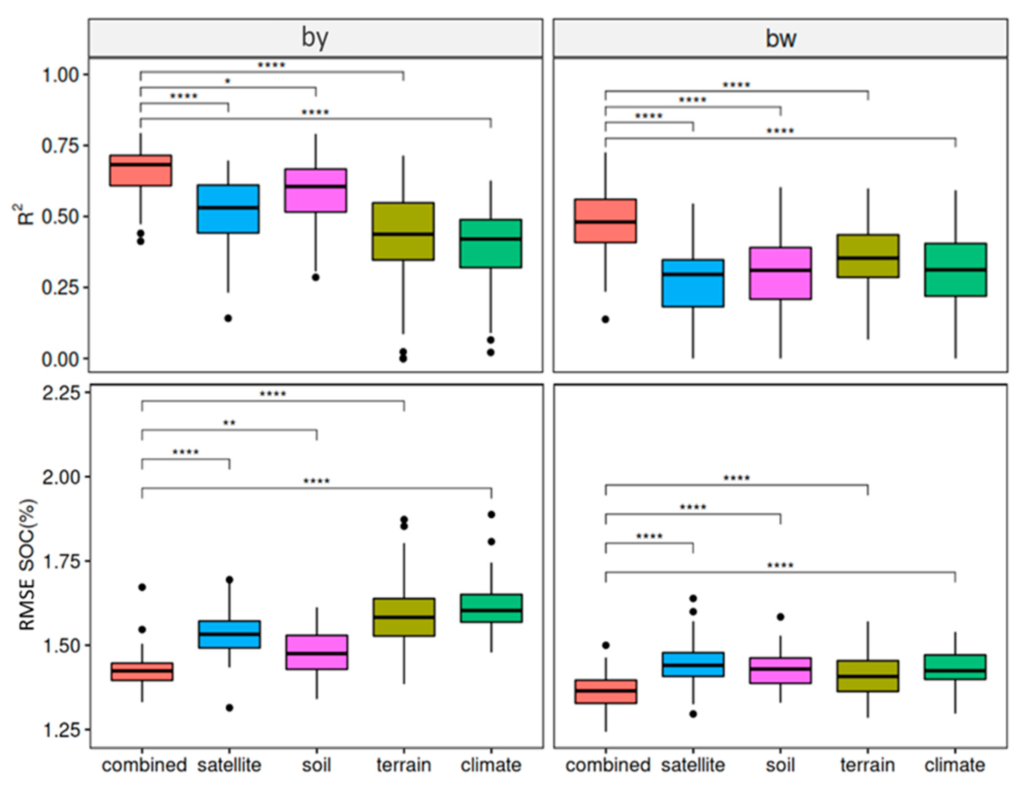
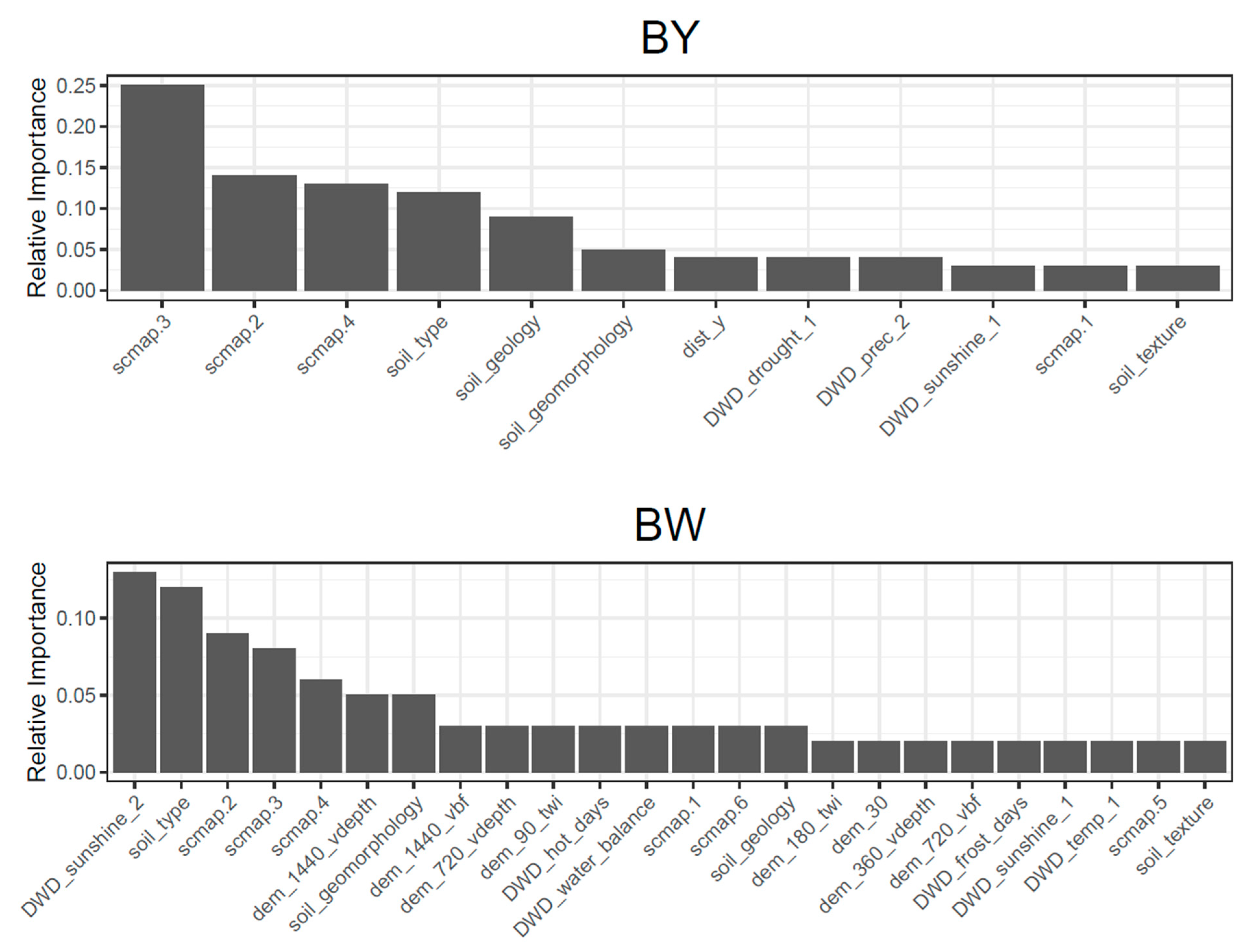
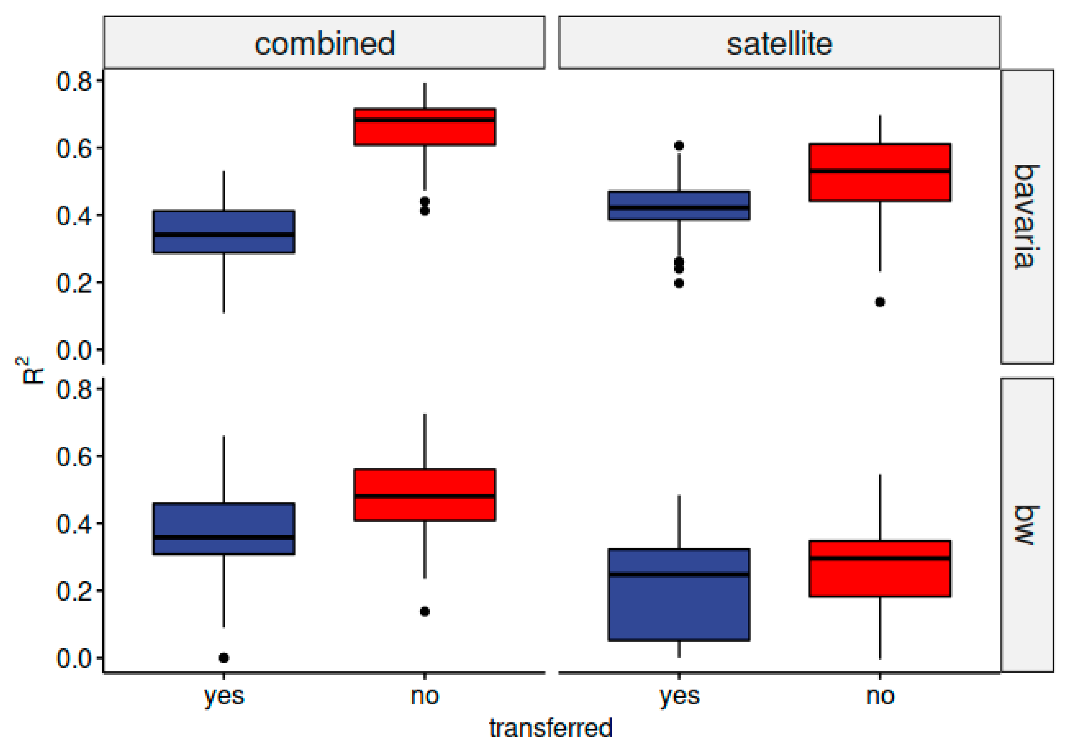
3.1. Performance of the Baseline Models
3.2. Performance of the Transferred Models
3.3. Performance of the Mixed Data Models
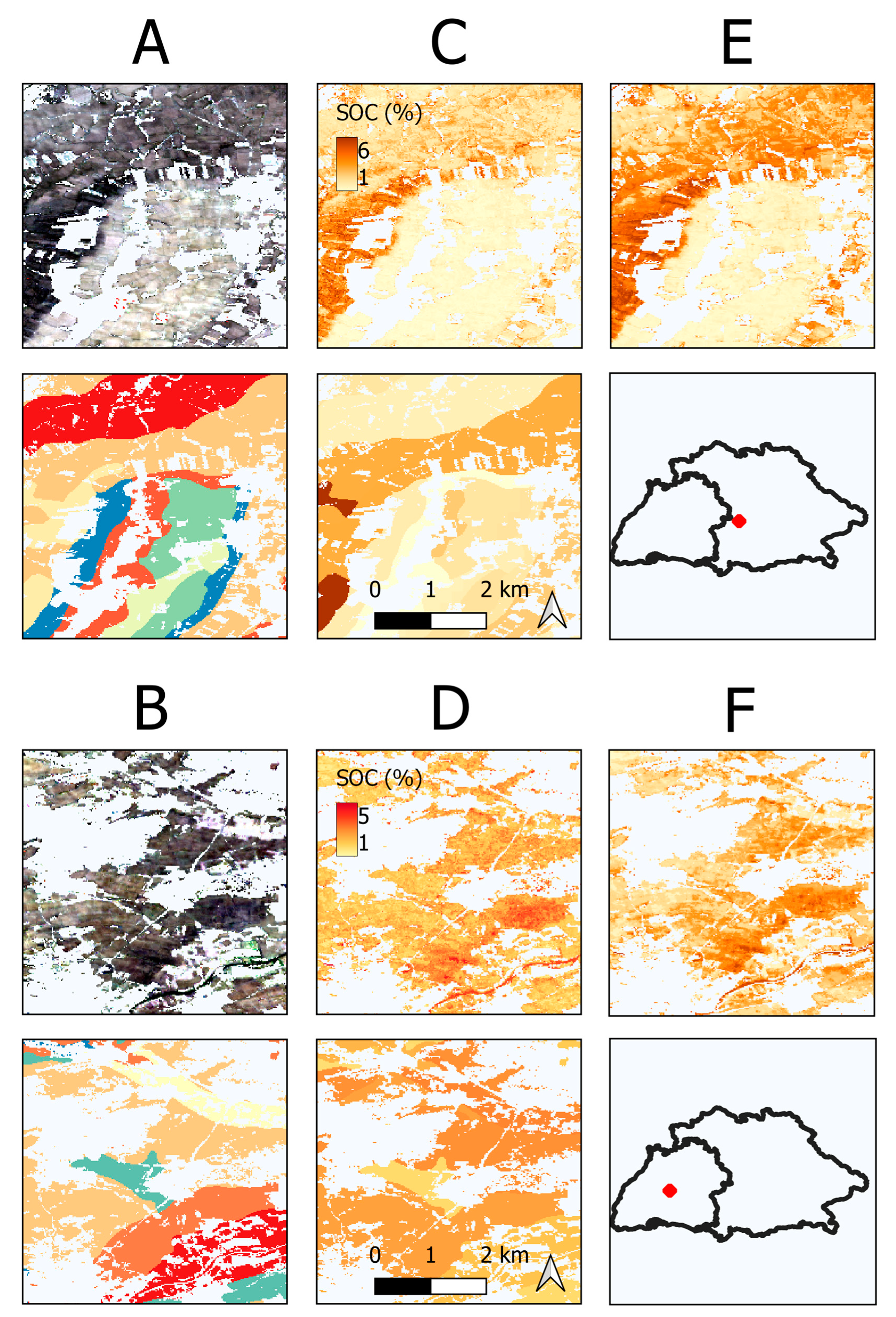
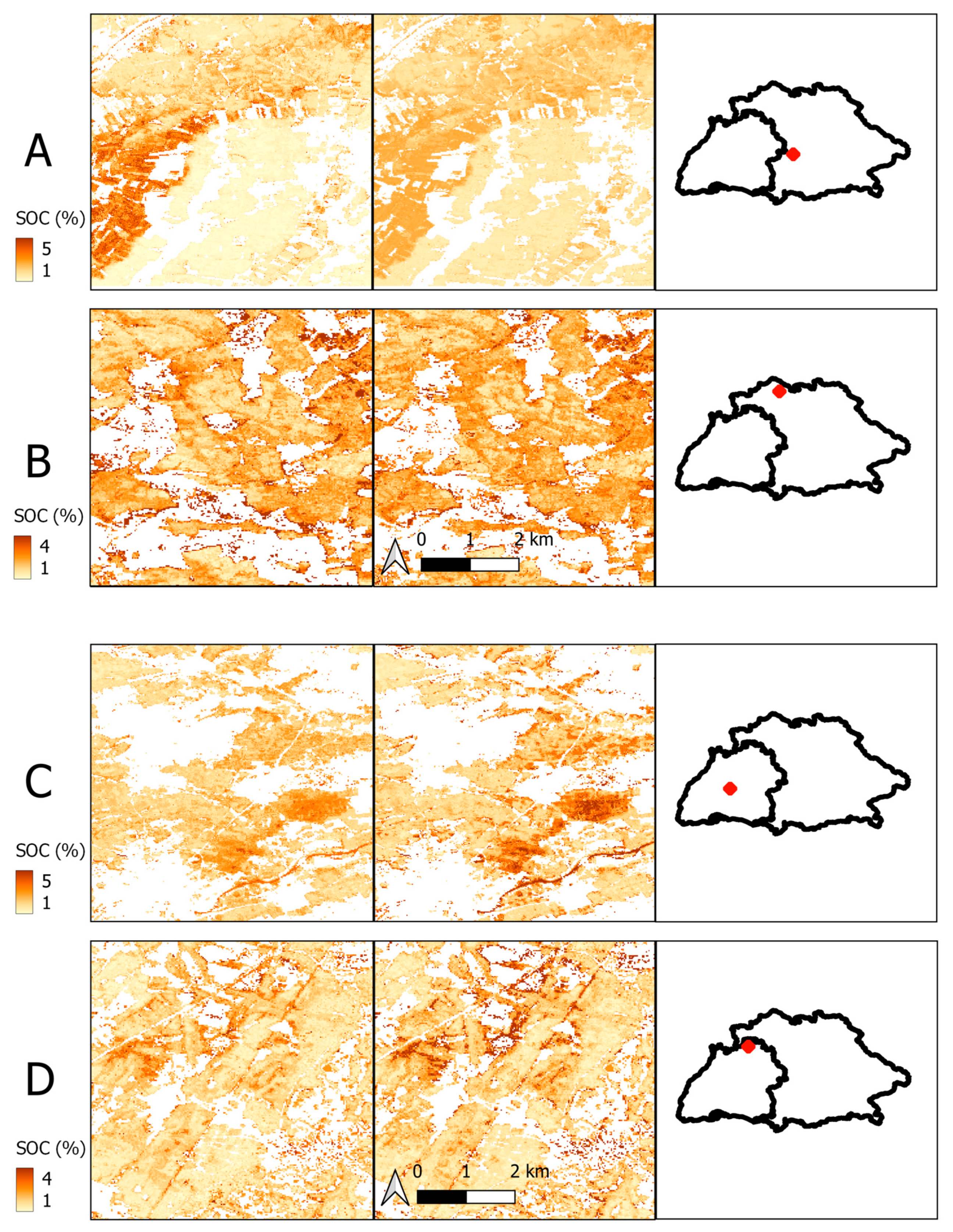
3.4. Final Prediction Maps
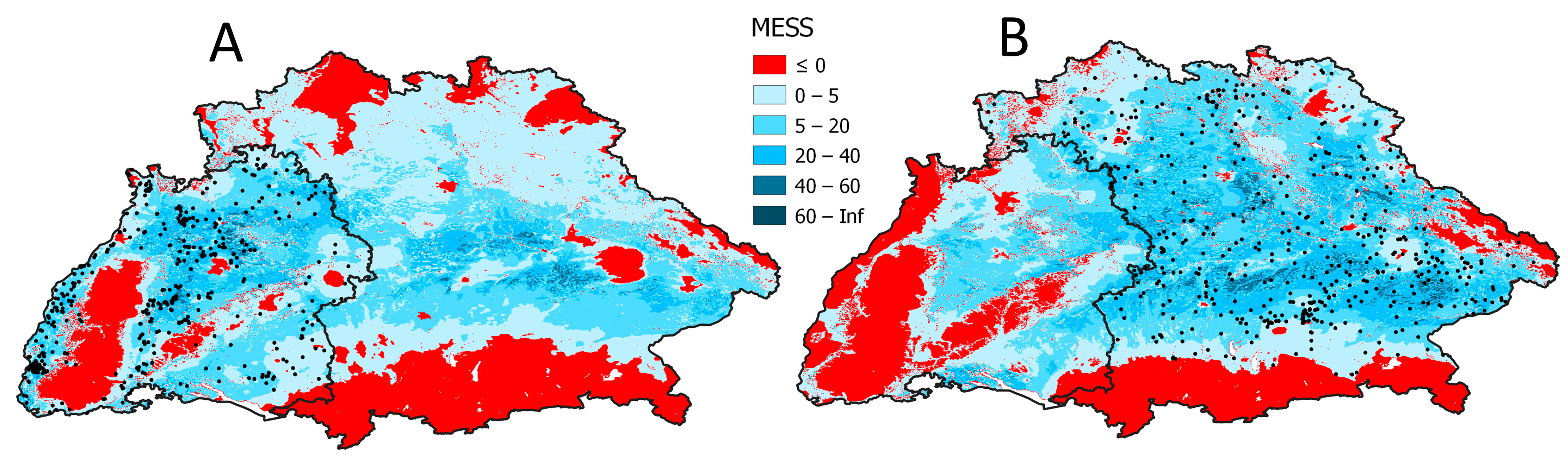
3.5. Similarity of the States
4. Discussion
4.1. General Model Performance
4.2. Differences between the States
4.3. Transferability of Different Covariate Groups
4.4. Limitations and Future Research
4.5. Recommendations for the Transfer and Extrapolation of SOC-Models
5. Conclusions
Author Contributions
Funding
Data Availability Statement
Acknowledgments
Conflicts of Interest
References
- Lal, R. Soil health and carbon management. Food Energy Secur. 2016, 5, 212–222. [Google Scholar] [CrossRef]
- Lal, R. Global potential of soil carbon sequestration to mitigate the greenhouse effect. Crit. Rev. Plant Sci. 2003, 22, 151–184. [Google Scholar] [CrossRef]
- Janzen, H.H. The soil carbon dilemma: Shall we hoard it or use it? Soil Biol. Biochem. 2006, 38, 419–424. [Google Scholar] [CrossRef]
- Smith, P.; Falloon, P.; Kutsch, W.L. The role of soils in the Kyoto Protocol. In Soil Carbon Dynamics: An Integrated Methodology; Cambridge University Press: Cambridge, UK, 2010; pp. 245–256. ISBN 9780511711794. [Google Scholar]
- Van Wesemael, B.; Chabrillat, S.; Wilken, F. High-spectral resolution remote sensing of soil organic carbon dynamics. Remote Sens. 2021, 13, 1293. [Google Scholar] [CrossRef]
- McBratney, A.B.; Mendonça Santos, M.L.; Minasny, B. On digital soil mapping. Geoderma 2003, 117, 3–52. [Google Scholar] [CrossRef]
- Taghizadeh-Mehrjardi, R.; Khademi, H.; Khayamim, F.; Zeraatpisheh, M.; Heung, B.; Scholten, T. A Comparison of Model Averaging Techniques to Predict the Spatial Distribution of Soil Properties. Remote Sens. 2022, 14, 472. [Google Scholar] [CrossRef]
- Hengl, T.; Nussbaum, M.; Wright, M.N.; Heuvelink, G.B.; Gräler, B. Random forest as a generic framework for predictive modeling of spatial and spatio-temporal variables. PeerJ 2018, 2018, e5518. [Google Scholar] [CrossRef]
- Fathizad, H.; Taghizadeh-Mehrjardi, R.; Hakimzadeh Ardakani, M.A.; Zeraatpisheh, M.; Heung, B.; Scholten, T. Spatiotemporal Assessment of Soil Organic Carbon Change Using Machine-Learning in Arid Regions. Agronomy 2022, 12, 628. [Google Scholar] [CrossRef]
- Taghizadeh-Mehrjardi, R.; Schmidt, K.; Amirian-Chakan, A.; Rentschler, T.; Zeraatpisheh, M.; Sarmadian, F.; Valavi, R.; Davatgar, N.; Behrens, T.; Scholten, T. Improving the spatial prediction of soil organic carbon content in two contrasting climatic regions by stacking machine learning models and rescanning covariate space. Remote Sens. 2020, 12, 1095. [Google Scholar] [CrossRef]
- Behrens, T.; Scholten, T. Chapter 25 A Comparison of Data-Mining Techniques in Predictive Soil Mapping. In Digital Soil Mapp.ing—An Introductory Perspective; Elsevier: Amsterdam, The Netherlands, 2006; pp. 353–617. ISBN 9780444529589. [Google Scholar]
- Rentschler, T.; Bartelheim, M.; Behrens, T.; Díaz-Zorita Bonilla, M.; Teuber, S.; Scholten, T.; Schmidt, K. Contextual spatial modelling in the horizontal and vertical domains. Sci. Rep. 2022, 12, 9496. [Google Scholar] [CrossRef]
- Emadi, M.; Taghizadeh-Mehrjardi, R.; Cherati, A.; Danesh, M.; Mosavi, A.; Scholten, T. Predicting and Mapp.ing of Soil Organic Carbon Using Machine Learning Algorithms in Northern Iran. Remote Sens. 2020, 12, 2234. [Google Scholar] [CrossRef]
- Rogge, D.; Bauer, A.; Zeidler, J.; Mueller, A.; Esch, T.; Heiden, U. Building an exposed soil composite processor (SCMaP) for mapp.ing spatial and temporal characteristics of soils with Landsat imagery (1984–2014). Remote Sens. Environ. 2018, 205, 1–17. [Google Scholar] [CrossRef]
- Diek, S.; Fornallaz, F.; Schaepman, M.E.; de Jong, R. Barest Pixel Composite for agricultural areas using landsat time series. Remote Sens. 2017, 9, 1245. [Google Scholar] [CrossRef]
- Demattê, J.A.; Safanelli, J.L.; Poppiel, R.R.; Rizzo, R.; Silvero, N.E.Q.; de Sousa Mendes, W.; Bonfatti, B.R.; Dotto, A.C.; Salazar, D.F.U.; de Oliveira Mello, F.A.; et al. Bare Earth’s Surface Spectra as a Proxy for Soil Resource Monitoring. Sci. Rep. 2020, 10, 4461. [Google Scholar] [CrossRef]
- Safanelli, J.L.; Chabrillat, S.; Ben-Dor, E.; Demattê, J.A. Multispectral models from bare soil composites for mapp.ing topsoil properties over Europe. Remote Sens. 2020, 12, 1369. [Google Scholar] [CrossRef]
- Vaudour, E.; Gomez, C.; Lagacherie, P.; Loiseau, T.; Baghdadi, N.; Urbina-Salazar, D.; Loubet, B.; Arrouays, D. Temporal mosaicking app.roaches of Sentinel-2 images for extending topsoil organic carbon content mapp.ing in croplands. Int. J. Appl. Earth Obs. Geoinf. 2021, 96, 102277. [Google Scholar] [CrossRef]
- Zepp, S.; Heiden, U.; Bachmann, M.; Wiesmeier, M.; Steininger, M.; van Wesemael, B. Estimation of soil organic carbon contents in croplands of bavaria from scmap soil reflectance composites. Remote Sens. 2021, 13, 3141. [Google Scholar] [CrossRef]
- Möller, M.; Zepp, S.; Wiesmeier, M.; Gerighausen, H.; Heiden, U. Scale-Specific Prediction of Topsoil Organic Carbon Contents Using Terrain Attributes and SCMaP Soil Reflectance Composites. Remote Sens. 2022, 14, 2295. [Google Scholar] [CrossRef]
- Maleki, S.; Khormali, F.; Mohammadi, J.; Bogaert, P.; Bagheri Bodaghabadi, M. Effect of the accuracy of topographic data on improving digital soil mapp.ing predictions with limited soil data: An app.lication to the Iranian loess plateau. CATENA 2020, 195, 10481. [Google Scholar] [CrossRef]
- Stumpf, F.; Schmidt, K.; Behrens, T.; Schönbrodt-Stitt, S.; Buzzo, G.; Dumperth, C.; Wadoux, A.; Xiang, W.; Scholten, T. Incorporating limited field operability and legacy soil samples in a hypercube sampling design for digital soil mapping. J. Plant Nutr. Soil Sci. 2016, 179, 499–509. [Google Scholar] [CrossRef]
- Gehl, R.J.; Rice, C.W. Emerging technologies for in situ measurement of soil carbon. Clim. Chang. 2007, 80, 43–54. [Google Scholar] [CrossRef]
- McKay, J.; Grunwald, S.; Shi, X.; Long, R.F. Evaluation of the Transferability of a Knowledge-Based Soil-Landscape Model. In Digital Soil Mapping; Springer: Berlin/Heidelberg, Germany, 2010; pp. 165–178. [Google Scholar]
- Malone, B.P.; Jha, S.K.; Minasny, B.; McBratney, A.B. Comparing regression-based digital soil mapp.ing and multiple-point geostatistics for the spatial extrapolation of soil data. Geoderma 2016, 262, 243–253. [Google Scholar] [CrossRef]
- De Arruda, G.P.; Demattê, J.; Chagas, C.; Fiorio, P.R.; e Souza, A.B.; Fongaro, C.T. Digital soil mapp.ing using reference area and artificial neural networks. Sci. Agric. 2016, 73, 266–273. [Google Scholar] [CrossRef]
- Wolski, M.S.; Dalmolin, R.S.D.; Flores, C.A.; Moura-Bueno, J.M.; ten Caten, A.; Kaiser, D.R. Digital soil mapp.ing and its implications in the extrapolation of soil-landscape relationships in detailed scale. Pesqui. Agropecu. Bras. 2017, 52, 633–642. [Google Scholar] [CrossRef]
- Zhao, Z.; Yang, Q.; Sun, D.; Ding, X.; Meng, F.R. Extended model prediction of high-resolution soil organic matter over a large area using limited number of field samples. Comput. Electron. Agric. 2020, 169, 105172. [Google Scholar] [CrossRef]
- Neyestani, M.; Sarmadian, F.; Jafari, A.; Keshavarzi, A.; Sharififar, A. Digital mapp.ing of soil classes using spatial extrapolation with imbalanced data. Geoderma Reg. 2021, 26, e00422. [Google Scholar] [CrossRef]
- Machado, D.F.T.; Silva, S.H.G.; Curi, N.; de Menezes, M.D. Soil type spatial prediction from random forest: Different training datasets, transferability, accuracy and uncertainty assessment. Sci. Agric. 2019, 76, 243–254. [Google Scholar] [CrossRef]
- Taghizadeh-Mehrjardi, R.; Sheikhpour, R.; Zeraatpisheh, M.; Amirian-Chakan, A.; Toomanian, N.; Kerry, R.; Scholten, T. Semi-supervised learning for the spatial extrapolation of soil information. Geoderma 2022, 426, 116094. [Google Scholar] [CrossRef]
- Hengl, T. Extrapolation is Tough for Trees (Tree-Based Learners), Combining Learners of Different Type Makes It Less Tough. 2021. Available online: https://medium.com/nerd-for-tech/extrapolation-is-tough-for-trees-tree-based-learners-combining-learners-of-different-type-makes-659187a6f58d (accessed on 19 December 2022).
- Zeraatpisheh, M.; Garosi, Y.; Reza Owliaie, H.; Ayoubi, S.; Taghizadeh-Mehrjardi, R.; Scholten, T.; Xu, M. Improving the spatial prediction of soil organic carbon using environmental covariates selection: A comparison of a group of environmental covariates. CATENA 2022, 208, 105723. [Google Scholar] [CrossRef]
- BGR. Geologische Übersichtskarte der Bundesrepublik Deutschland 1: 200 000 (GÜK200). 2021. Available online: https://www.bgr.bund.de/DE/Themen/Sammlungen-Grundlagen/GG_geol_Info/Karten/Deutschland/GUEK200/guek200_inhalt.html (accessed on 19 December 2022).
- BGR. Bodenübersichtskarte 1:200.000 (BÜK200). 2018. Available online: https://www.bgr.bund.de/DE/Themen/Boden/Informationsgrundlagen/Bodenkundliche_Karten_Datenbanken/BUEK200/buek200_node.html (accessed on 19 December 2022).
- Jones, A.; Fernández-Ugalde, O.; Scarpa, S. LUCAS 2015 Topsoil Survey: Presentation of Dataset and Results; Publications Office of the European Union: Luxembourg, 2020; ISBN 9789276210801. [Google Scholar]
- GDAL/OGR Contributors. {GDAL/OGR} Geospatial Data Abstraction Software Library. 2022. Available online: https://gdal.org (accessed on 19 December 2022).
- Behrens, T.; Schmidt, K.; Viscarra Rossel, R.A.; Gries, P.; Scholten, T.; MacMillan, R.A. Spatial modelling with Euclidean distance fields and machine learning. Eur. J. Soil Sci. 2018, 69, 757–770. [Google Scholar] [CrossRef]
- Møller, A.B.; Beucher, A.M.; Pouladi, N.; Greve, M.H. Oblique geographic coordinates as covariates for digital soil mapping. SOIL 2020, 6, 269–289. [Google Scholar] [CrossRef]
- Zepp, S.; Jilge, M.; Metz-Marconcini, A.; Heiden, U. The influence of vegetation index thresholding on EO-based assessments of exposed soil masks in Germany between 1984 and 2019. ISPRS J. Photogramm. Remote Sens. 2021, 178, 366–381. [Google Scholar] [CrossRef]
- JAXA EORC. ALOS Global Digital Surface Model (DSM). ALOS World, 2021; 1.2, 1–21.
- Conrad, O.; Bechtel, B.; Bock, M.; Dietrich, H.; Fischer, E.; Gerlitz, L.; Wehberg, J.; Wichmann, V.; Böhner, J. System for Automated Geoscientific Analyses (SAGA) v. 2.1.4. Geosci. Model Dev. 2015, 8, 1991–2007. [Google Scholar] [CrossRef]
- Hengl, T.; MacMillan, R.A. Predictive Soil Mapping with R; OpenGeoHub Foundation: Wageningen, The Netherlands, 2019; pp. 1–370. ISBN 978-0-359-30635-0. [Google Scholar]
- Behrens, T.; Schmidt, K.; MacMillan, R.A.; Viscarra Rossel, R.A. Multiscale contextual spatial modelling with the Gaussian scale space. Geoderma 2018, 310, 128–137. [Google Scholar] [CrossRef]
- Deutscher Wetterdienst. Open-Data-Server des Deutschen Wetterdienstes (DWD). 2022. Available online: https://opendata.dwd.de/ (accessed on 19 December 2022).
- Hengl, T. GSIF: Global Soil Information Facilities. 2020. Available online: https://CRAN.R-project.org/package=GSIF (accessed on 19 December 2022).
- BGR. Gruppen der Bodenausgangsgesteine 1:5.000.000 (BAG5000). 2007. Available online: https://www.bgr.bund.de/DE/Themen/Boden/Informationsgrundlagen/Bodenkundliche_Karten_Datenbanken/Themenkarten/BAG5000/bag5000_node.html (accessed on 19 December 2022).
- BGR. Geomorphographische Einheiten der Bundesrepublik Deutschland. 2001. Available online: https://www.bgr.bund.de/DE/Themen/Boden/Bilder/Bod_Neuausrichtung_Bodenkartierung_abb1_g_720.html (accessed on 19 December 2022).
- Ad-hoc-Arbeitsgruppe Boden. Bodenkundliche Kartieranleitung KA5; Schweizerbart Science Publishers: Stuttgart, Germany, 2006; ISBN 9783510959204. [Google Scholar]
- Elith, J.; Phillips, S.J.; Hastie, T.; Dudík, M.; Chee, Y.E.; Yates, C.J. A statistical explanation of MaxEnt for ecologists. Divers. Distrib. 2011, 17, 43–57. [Google Scholar] [CrossRef]
- Meyer, H.; Pebesma, E. Predicting into unknown space? Estimating the area of applicability of spatial prediction models. Methods Ecol. Evol. 2021, 12, 1620–1633. [Google Scholar] [CrossRef]
- Breiman, L. Random Forests. Mach. Learn. 2001, 45, 5–32. [Google Scholar] [CrossRef]
- Breiman, L. Statistical Modeling: The Two Cultures. Stat. Sci. 2001, 16, 199–231. [Google Scholar] [CrossRef]
- LeDell, E.; Gill, N.; Aiello, S.; Fu, A.; Candel, A.; Click, C.; Kraljevic, T.; Nykodym, T.; Aboyoun, P.; Kurka, M.; et al. h2o: R Interface for the ‘H2O’ Scalable Machine Learning Platform. 2021. Available online: https://CRAN.R-project.org/package=h2o (accessed on 19 December 2022).
- Kassambara, A. ggpubr: ‘ggplot2’ Based Publication Ready Plots. 2020. Available online: https://cran.r-project.org/package=ggpubr (accessed on 19 December 2022).
- Wright, M.N.; Ziegler, A. Ranger: A Fast Implementation of Random Forests for High Dimensional Data in C++ and R. J. Stat. Soft. 2017, 77, 1–17. [Google Scholar] [CrossRef]
- Vaudour, E.; Gholizadeh, A.; Castaldi, F.; Saberioon, M.; Borůvka, L.; Urbina-Salazar, D.; Fouad, Y.; Arrouays, D.; Richer-de-Forges, A.C.; Biney, J.; et al. Satellite Imagery to Map Topsoil Organic Carbon Content over Cultivated Areas: An Overview. Remote Sens. 2022, 14, 2917. [Google Scholar] [CrossRef]
- Dvorakova, K.; Heiden, U.; van Wesemael, B. Sentinel-2 Exposed Soil Composite for Soil Organic Carbon Prediction. Remote Sens. 2021, 13, 1791. [Google Scholar] [CrossRef]
- Urbina-Salazar, D.; Vaudour, E.; Baghdadi, N.; Ceschia, E.; Richer-de-Forges, A.C.; Lehmann, S.; Arrouays, D. Using Sentinel-2 Images for Soil Organic Carbon Content Mapping in Croplands of Southwestern France. The Usefulness of Sentinel-1/2 Derived Moisture Maps and Mismatches between Sentinel Images and Sampling Dates. Remote Sens. 2021, 13, 5115. [Google Scholar] [CrossRef]
- Žížala, D.; Minařík, R.; Zádorová, T. Soil Organic Carbon Mapp.ing Using Multispectral Remote Sensing Data: Prediction Ability of Data with Different Spatial and Spectral Resolutions. Remote Sens. 2019, 11, 2947. [Google Scholar] [CrossRef]
- Bonannella, C.; Hengl, T.; Heisig, J.; Parente, L.; Wright, M.N.; Herold, M.; de Bruin, S. Forest tree species distribution for Europe 2000–2020: Mapping potential and realized distributions using spatiotemporal machine learning. PeerJ 2022, 10, e13728. [Google Scholar] [CrossRef] [PubMed]
- Fathololoumi, S.; Vaezi, A.R.; Alavipanah, S.K.; Ghorbani, A.; Saurette, D.; Biswas, A. Improved digital soil mapp.ing with multitemporal remotely sensed satellite data fusion: A case study in Iran. Sci. Total Environ. 2020, 721, 137703. [Google Scholar] [CrossRef] [PubMed]
- Minasny, B.; McBratney, A. Why calculating RPD is redundant. Pedometron 2013, 33, 14–15. [Google Scholar]
- Wiesmeier, M.; Hübner, R.; Barthold, F.; Spörlein, P.; Geuß, U.; Hangen, E.; Reischl, A.; Schilling, B.; von Lützow, M.; Kögel-Knabner, I. Amount, distribution and driving factors of soil organic carbon and nitrogen in cropland and grassland soils of southeast Germany (Bavaria). Agric. Ecosyst. Environ. 2013, 176, 39–52. [Google Scholar] [CrossRef]
- Ma, T.; Brus, D.J.; Zhu, A.-X.; Zhang, L.; Scholten, T. Comparison of conditioned Latin hypercube and feature space coverage sampling for predicting soil classes using simulation from soil maps. Geoderma 2020, 370, 114366. [Google Scholar] [CrossRef]
- Meyer, H.; Reudenbach, C.; Hengl, T.; Katurji, M.; Nauss, T. Improving performance of spatio-temporal machine learning models using forward feature selection and target-oriented validation. Environ. Model. Softw. 2018, 101, 1–9. [Google Scholar] [CrossRef]
- Castaldi, F.; Chabrillat, S.; Don, A.; van Wesemael, B. Soil organic carbon mapp.ing using LUCAS topsoil database and Sentinel-2 data: An app.roach to reduce soil moisture and crop residue effects. Remote Sens. 2019, 11, 2121. [Google Scholar] [CrossRef]
- Dvorakova, K.; Shi, P.; Limbourg, Q.; van Wesemael, B. Soil Organic Carbon Mapping from Remote Sensing: The Effect of Crop Residues. Remote Sens. 2020, 12, 1913. [Google Scholar] [CrossRef]
- Guo, L.; Sun, X.; Fu, P.; Shi, T.; Dang, L.; Chen, Y.; Linderman, M.; Zhang, G.; Zhang, Y.; Jiang, Q.; et al. Mapp.ing soil organic carbon stock by hyperspectral and time-series multispectral remote sensing images in low-relief agricultural areas. Geoderma 2021, 398, 115118. [Google Scholar] [CrossRef]
- Guanter, L.; Kaufmann, H.; Foerster, S.; Brosinsky, A.; Wulf, H.; Bochow, M.; Boesche, N.; Brell, M.; Buddenbaum, H.; Chabrillat, S.; et al. Environmental Mapping and Analysis Program (EnMAP) EnMAP Science Plan 2016; EnMAP Consortium: Potsdam, Germany, 2016. [Google Scholar] [CrossRef]
- Jacobs, A.; Flessa, H.; Don, A.; Heidkamp, A.; Prietz, R.; Dechow, R.; Gensior, A.; Poeplau, C.; Riggers, C.; Schneider, F.; et al. Landwirtschaftlich genutzte Böden in Deutschland: Ergebnisse der Bodenzustandserhebung; Thünen Report No. 64.; Johann Heinrich von Thünen-Institut: Braunschweig, Germany, 2018; Volume 64. [Google Scholar] [CrossRef]
- Vohland, M.; Ludwig, B.; Seidel, M.; Hutengs, C. Quantification of soil organic carbon at regional scale: Benefits of fusing vis-NIR and MIR diffuse reflectance data are greater for in situ than for laboratory-based modelling approaches. Geoderma 2022, 405, 115426. [Google Scholar] [CrossRef]
- Gholizadeh, A.; Neumann, C.; Chabrillat, S.; van Wesemael, B.; Castaldi, F.; Borůvka, L.; Sanderman, J.; Klement, A.; Hohmann, C. Soil organic carbon estimation using VNIR–SWIR spectroscopy: The effect of multiple sensors and scanning conditions. Soil Tillage Res. 2021, 211, 105017. [Google Scholar] [CrossRef]
- Hong, Y.; Chen, S.; Chen, Y.; Linderman, M.; Mouazen, A.M.; Liu, Y.; Guo, L.; Yu, L.; Liu, Y.; Cheng, H.; et al. Comparing laboratory and airborne hyperspectral data for the estimation and mapping of topsoil organic carbon: Feature selection coupled with random forest. Soil Tillage Res. 2020, 199, 104589. [Google Scholar] [CrossRef]
- Hengl, T.; Parente, L.; Bouasria, A.; Wheeler, I. Spatial Sampling and Resampling for Machine Learning; Zenodo: Geneva, Switzerland, 2022. [Google Scholar] [CrossRef]
- Sakhaee, A.; Gebauer, A.; Ließ, M.; Don, A. Spatial prediction of organic carbon in German agricultural topsoil using machine learning algorithms. SOIL 2022, 8, 587–604. [Google Scholar] [CrossRef]
- Roudier, P.; Odgers, N.; Carrick, S.; Eger, A.; Hainsworth, S.; Beaudette, D. Soilscapes of New Zealand: Pedologic diversity as organised along environmental gradients. Geoderma 2022, 409, 115637. [Google Scholar] [CrossRef]


| Bavaria | Baden-Wuerttemberg | |
|---|---|---|
| Area (km2) | 71,000 | 36,000 |
| Area of cropland soils (km2) | 34,000 | 11,000 |
| Proportion of cropland to total area (%) | 48 | 31 |
| Mean temperature (°C) | 8.7 | 10 |
| Mean precipitations (mm) | 836 | 818 |
| Predominant soil type | Cambisol | Luvisol |
| State | Source | Samples | SOC (%) | SOC (%) | SOC (%) | SOC (%) | SOC (%) |
|---|---|---|---|---|---|---|---|
| Min | Max | Mean | SD | IQR | |||
| BY | LUCAS | 227 | 0.6 | 14.81 | 2.1 | 1.68 | 1.15 |
| LfU | 248 | 0.54 | 15.6 | 3.13 | 2.8 | 1.91 | |
| Total | 475 | 0.54 | 15.6 | 2.63 | 2.38 | 1.54 | |
| BW | LUCAS | 91 | 0.79 | 5.78 | 1.78 | 0.87 | 0.99 |
| LGRB | 384 | 0.45 | 8.31 | 1.48 | 0.93 | 0.88 | |
| Total | 475 | 0.45 | 8.31 | 1.74 | 0.92 | 0.9 |
| Soil Type | BY | BW | |||
|---|---|---|---|---|---|
| German Soil System | World Reference Base | Samples | Mean SOC (%) | Samples | Mean SOC (%) |
| Vega | Fluvisols | 26 | 2.69 | 66 | 1.67 |
| Braunerde | Cambisols | 217 | 1.64 | 70 | 2.1 |
| Pelosol | Vertisols | 26 | 1.96 | 31 | 2.72 |
| Gley | Gleysols | 53 | 3.44 | 22 | 2.66 |
| Anmoorgley | Gleysols | 37 | 8.76 | 1 | 3.57 |
| Parabraunerde | Luvisols | 35 | 1.77 | 201 | 1.37 |
| Rendzina | Leptosols | 14 | 3.14 | 24 | 2.23 |
| Pararendzina | Regosols | 44 | 2.77 | 52 | 1.64 |
| Pseudogley | Planosols | 15 | 2.02 | 1 | 1.16 |
| Kolluvisol | Colluvic | 8 | 1.34 | 7 | 1.47 |
| Baseline Models | Transferred Models | |||||||||
|---|---|---|---|---|---|---|---|---|---|---|
| Group | R2 | RMSE | CCC | MAE | OOB | R2 | RMSE | CCC | MAE | |
| BY | combined | 0.68 | 1.42 | 0.81 | 0.74 | 1.93 | 0.34 | 1.68 | 0.47 | 0.57 |
| satellite | 0.53 | 1.53 | 0.71 | 0.88 | 2.69 | 0.42 | 1.63 | 0.5 | 0.58 | |
| soil | 0.61 | 1.48 | 0.77 | 0.79 | 1.97 | 0 | 1.91 | 0 | 0.76 | |
| terrain | 0.44 | 1.58 | 0.63 | 0.96 | 3.18 | 0 | 2.01 | 0 | 0.87 | |
| climate | 0.42 | 1.6 | 0.61 | 0.92 | 3.31 | 0 | 1.99 | 0 | 1.2 | |
| BW | combined | 0.48 | 1.37 | 0.63 | 0.44 | 0.4 | 0.36 | 1.43 | 0.44 | 0.91 |
| satellite | 0.3 | 1.44 | 0.48 | 0.52 | 0.53 | 0.25 | 1.50 | 0.41 | 0.87 | |
| soil | 0.31 | 1.43 | 0.5 | 0.49 | 0.51 | 0 | 1.64 | 0 | 1.15 | |
| terrain | 0.35 | 1.41 | 0.54 | 0.51 | 0.50 | 0 | 1.60 | 0 | 1.11 | |
| climate | 0.31 | 1.43 | 0.5 | 0.54 | 0.52 | 0 | 1.62 | 0 | 1.22 | |
Disclaimer/Publisher’s Note: The statements, opinions and data contained in all publications are solely those of the individual author(s) and contributor(s) and not of MDPI and/or the editor(s). MDPI and/or the editor(s) disclaim responsibility for any injury to people or property resulting from any ideas, methods, instructions or products referred to in the content. |
© 2023 by the authors. Licensee MDPI, Basel, Switzerland. This article is an open access article distributed under the terms and conditions of the Creative Commons Attribution (CC BY) license (https://creativecommons.org/licenses/by/4.0/).
Share and Cite
Broeg, T.; Blaschek, M.; Seitz, S.; Taghizadeh-Mehrjardi, R.; Zepp, S.; Scholten, T. Transferability of Covariates to Predict Soil Organic Carbon in Cropland Soils. Remote Sens. 2023, 15, 876. https://doi.org/10.3390/rs15040876
Broeg T, Blaschek M, Seitz S, Taghizadeh-Mehrjardi R, Zepp S, Scholten T. Transferability of Covariates to Predict Soil Organic Carbon in Cropland Soils. Remote Sensing. 2023; 15(4):876. https://doi.org/10.3390/rs15040876
Chicago/Turabian StyleBroeg, Tom, Michael Blaschek, Steffen Seitz, Ruhollah Taghizadeh-Mehrjardi, Simone Zepp, and Thomas Scholten. 2023. "Transferability of Covariates to Predict Soil Organic Carbon in Cropland Soils" Remote Sensing 15, no. 4: 876. https://doi.org/10.3390/rs15040876