A CNN-LSTM Model for Soil Organic Carbon Content Prediction with Long Time Series of MODIS-Based Phenological Variables

Abstract

The spatial distribution of soil organic carbon (SOC) serves as critical geographic information for assessing ecosystem services, climate change mitigation, and optimal agriculture management. Digital mapping of SOC is challenging due to the complex relationships between the soil and its environment. Except for the well-known terrain and climate environmental covariates, vegetation that interacts with soils influences SOC significantly over long periods. Although several remote-sensing-based vegetation indices have been widely adopted in digital soil mapping, variables indicating long term vegetation growth have been less used. Vegetation phenology, an indicator of vegetation growth characteristics, can be used as a potential time series environmental covariate for SOC prediction. A CNN-LSTM model was developed for SOC prediction with inputs of static and dynamic environmental variables in Xuancheng City, China. The spatially contextual features in static variables (e.g., topographic variables) were extracted by the convolutional neural network (CNN), while the temporal features in dynamic variables (e.g., vegetation phenology over a long period of time) were extracted by a long short-term memory (LSTM) network. The ten-year phenological variables derived from moderate-resolution imaging spectroradiometer (MODIS) observations were adopted as predictors with historical temporal changes in vegetation in addition to the commonly used static variables. The random forest (RF) model was used as a reference model for comparison. Our results indicate that adding phenological variables can produce a more accurate map, as tested by the five-fold cross-validation, and demonstrate that CNN-LSTM is a potentially effective model for predicting SOC at a regional spatial scale with long-term historical vegetation phenology information as an extra input. We highlight the great potential of hybrid deep learning models, which can simultaneously extract spatial and temporal features from different types of environmental variables, for future applications in digital soil mapping.

1. Introduction

Soil organic carbon (SOC) accounts for two-thirds of the terrestrial ecosystem carbon [1,2]. Soil carbon plays a core role in the soil fertility that ensures soil health and crop yields, and an increment in its stocks can mitigate the greenhouse gas emissions affecting climate change [3,4,5,6]. However, soils in complicated landscapes interacting with human activities possess a large spatial heterogeneity in soil carbon [7,8]. Exploring the spatial distribution of SOC and identifying the drivers of its spatial variations are necessary and important to sustain biodiversity conservation and guide optimal agriculture management [9].

Recently, digital soil mapping (DSM) has become a popular approach for predicting the spatial distribution of soil organic carbon content with the support of a large amount of remote sensing data [10,11,12,13]. Because soil is influenced by its environmental factors, DSM is applied to predict soil types/properties through the relationships between soil and its environmental factors, constructed based on soil samples or expert knowledge [10]. The climate, terrain, and vegetation all affect the spatial distribution of soil properties (e.g., SOC). Furthermore, vegetation could have more interactions with soil than the other factors in some cases [14,15]. Soil fertility affects the growth of vegetation, and the carbon inputs to soil are significantly influenced by plant production. Studies have also suggested that vegetation growth could indicate agricultural management and is thus very useful for SOC prediction [16,17]. Therefore, vegetation indices obtained through remote sensing, such as the normalized difference vegetation index (NDVI) and enhanced vegetation index (EVI), have been increasingly used and are becoming a key covariate in soil carbon mapping [12,17,18].

In addition to vegetation indices representing vegetation growth conditions at single dates, there is an increasing interest in adoption of long time series of vegetation growth status due to the dynamic characteristic of vegetation over time. Recent studies have shown that vegetation information for a long period has a higher impact on soil carbon than that of a single year [19,20,21]. Plant phenology indicates the biological phenomena of vegetation growth, including the start of season, the end of season, the length of growing season, etc. [22,23]. Researchers have shown that phenology is strongly related to soil carbon [24,25,26,27,28]. For instance, with earlier spring warming, more days can be used for plant carbon uptake [29]. When a warming temperature prolongs the growing season, the organic carbon loss caused by soil respiration can be greater than that stored through plant photosynthesis [28]. Traditionally, plant phenology indicates the timing of life cycle events of plant species, but with the development of remote sensing techniques, it has been extended to a more generalized concept of land surface phenology (LSP). LSP is concerned with the seasonality of the reflectance characteristics of the stages of vegetation growth. Compared with traditional ground-based observations, it contains more abundant phenological features that are derived from the local to global coverage of long time series of remote sensing data [22]. Therefore, long time series of LSP data could potentially be used for improving the estimation of the spatial distribution of SOC.

SOC mapping usually relies on establishing a soil–environmental relationship. The commonly used environmental covariates, such as the mean annual climate and topographic variables, contain spatially contextual information. In addition, some covariates also change over time, such as phenological observations and vegetation indices, which can provide temporal features relating to soil organic carbon. Numerous methods, such as random forest [12,18,30], support vector machine [31,32], and regression kriging [33], have been successfully applied in DSM over the past decades. However, these methods mostly fit the relationship based on the soil and covariate data at sample locations. They still lack the ability to directly process the input data in both spatial and temporal structures. Therefore, it is necessary to develop new methods to take advantage of both the spatial and temporal features included in different types of environmental variables for DSM.

In recent years, deep learning has been applied successfully in many fields, including image classification and time series analysis [34,35] as well as dealing with the remote-sensing-based geographical problems [36,37,38,39]. The crucial superiority of deep learning is that it directly extracts the simple to abstract features of an object based on raw data [40] and is able to process spatial, temporal, and multi-dimensional data. Thus, deep learning provides an opportunity to simultaneously deal with different types of environmental variables for DSM. The convolutional neural network (CNN) [41] and long short-term memory (LSTM) [42] are two widely used network architectures in deep learning for dealing with data in the spatial domain and temporal domain, respectively [35]. Recently, CNN has been used for DSM in several studies. For example, Padarian et al. (2019) and Wadoux et al. (2019) used CNN and remote-sensing-derived environmental data to recognize the contextual information of environmental variables for multiple soil property predictions [43,44]. Some studies employed LSTM to estimate soil properties based on the input of hyperspectral data that can be considered as a kind of sequential data [45,46]. There are also studies that used LSTM to map soil moisture or soil temperature [47,48]. To our best knowledge, it is still rare in DSM and remote sensing communities to combine CNN and LSTM to deal with both spatial data and long time series of phenological information to improve SOC prediction.

In this study, we developed a deep learning model by combining CNN and LSTM for the predictive mapping of SOC. In addition to using the commonly used environmental variables, such as climate and topography, remote-sensing-based phenological variables over the ten years before the sampling year were adopted as an input for training the model. The objectives of this paper are: (1) to develop and evaluate the CNN-LSTM model for SOC prediction in a study area in Xuancheng city, China; (2) to evaluate the effectiveness of a long time series of phenological data in improving SOC prediction; and (3) to evaluate the performance of different groups of environmental variables for predicting SOC.

2. Study Area and Datasets

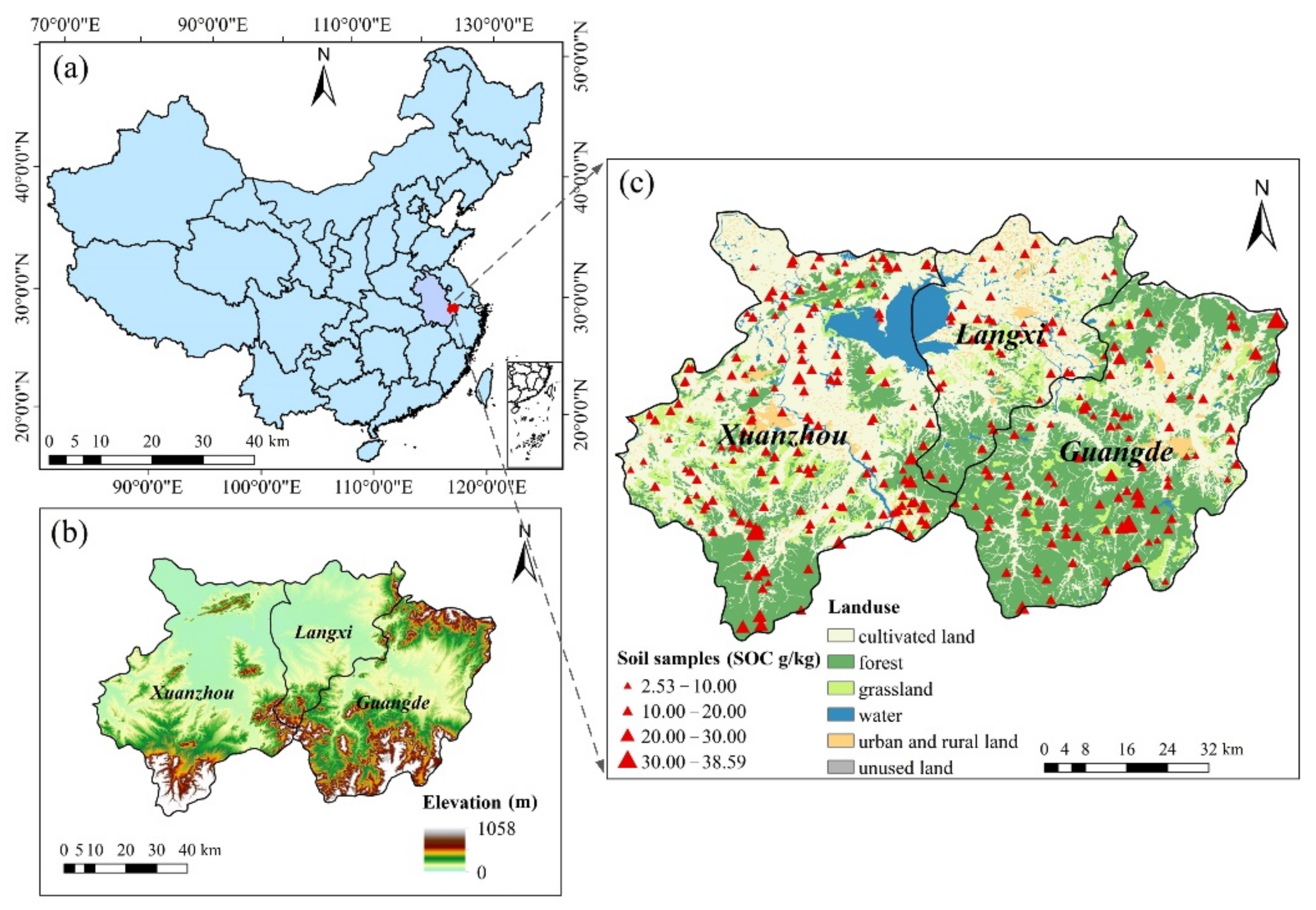
2.1. Study Area

The study area is located in Xuancheng City, Anhui Province, China (Figure 1), covering an area of 5568 km². The area has a subtropical humid monsoon climate [49]. The average annual precipitation is 1243 mm, and the average annual temperature is ~17 °C. The elevation of the area is between 0 and 1058 m, with a lower flat plain in the northwest, higher mountains in the south, and valleys in the northeast. According to the Chinese genetic soil classification system, red soil and paddy soil are the main soil types in the study area. The study area is mainly covered by cultivated land with various crops, such as rice, wheat, oilseed rape, and forest [50].

2.2. Soil Samples

A total of 308 samples were collected in the study area in 2011 through five sampling strategies, including integrative hierarchical stepwise sampling (59 samples), expert knowledge sampling (63 samples), systematic sampling (61 samples), heuristic uncertainty-directed sampling (61 samples), and stratified random sampling (64 samples) [15,50]. These soil samples cover the environmental characteristics of the study area well. The soil samples at these locations were collected at depths of 0–20 cm, and the SOC content (g/kg) of each sample was measured using the dichromate oxidation method [51].

2.3. Environmental Covariates

2.3.1. Climate and Topographic Data

We used ten variables to represent the climate and topography in the study area (

Table 1. Description of environmental covariates adopted in the study area.

Category	Variable Name	Variable Abbreviation	Spatial Resolution
Climate	Mean annual temperature	temp	1000 m
	Mean annual precipitation	preci
Terrain	Elevation	elev	90 m
	Slope	slp
	Terrain ruggedness index	tri
	Roughness	rough
	Vector ruggedness measure	vrm
	Topographic position index	tpi
	Compound topographic index	cti
	Stream power index	spi
Phenology	Date when EVI2 first crossed 15% of the segment EVI2 amplitude	greenup	500 m
	Date when EVI2 first crossed 50% of the segment EVI2 amplitude	mid-greenup
	Date when EVI2 first crossed 90% of the segment EVI2 amplitude	maturity
	Date when EVI2 reached the segment maximum	peak
	Date when EVI2 last crossed 90% of the segment EVI2 amplitude	senescence
	Date when EVI2 last crossed 50% of the segment EVI2 amplitude	mid-greendown
	Date when EVI2 last crossed 15% of the segment EVI2 amplitude	dormancy
	Total number of valid vegetation cycles with peak in product year	num-cycles
	Segment maximum–minimum EVI2	evi-amplitude
	Sum of daily interpolated EVI2 from Greenup to Dormancy	evi-area
	Segment minimum EVI2 value	evi-minimum
Vegetation index	Mean annual enhanced vegetation index	evi-mean	500 m

Note: EVI2, two-band enhanced vegetation index (EVI2) calculated from MODIS nadir bidirectional reflectance distribution function (BRDF)-adjusted reflectance (NBAR).

). The mean annual temperature (temp) and precipitation (preci) reported at WorldClim (http://worldclim.org, accessed on 1 November 2021) [52] were obtained to represent the climate condition of the area. Eight topographical variables, including elevation (elev), slope (slp), the terrain ruggedness index (tri), roughness (rough), the vector ruggedness measure (vrm), the topographic position index (tpi), the compound topographic index (cti), and the stream power index (spi), were obtained from the Geomorpho90m global dataset [53]. To be consistent with the spatial resolution of the digital elevation model (DEM), the climate data were interpolated to 90 m. All variables were reprojected to the WGS 1984 UTM 50N projection system.

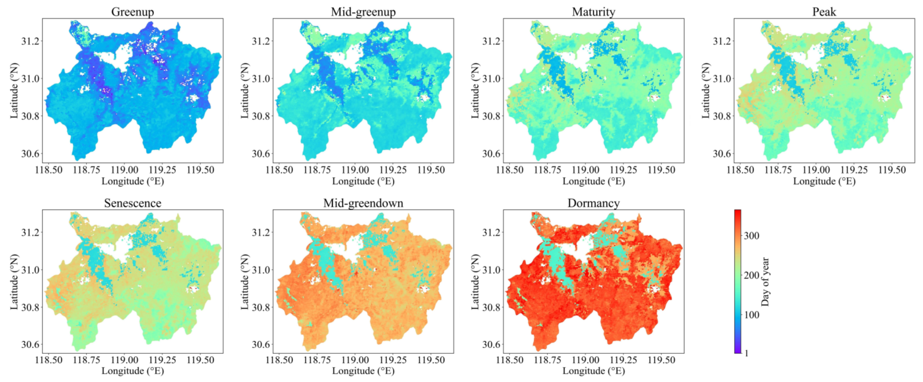
2.3.2. MODIS Land Surface Phenology Data

Several satellite sensors, such as the Moderate-Resolution Imaging Spectroradiometer (MODIS), Landsat, the Advanced Very High Resolution Radiometer (AVHRR), have been used for studies of LSP, with MODIS being the most-used satellite data source [22]. The global LSP metrics are provided by the MODIS land cover dynamics product (MCD12Q2) from 2000 and are based on time series of land surface greenness at a spatial resolution of 500 m [54]. This product has been well-validated [55,56]. The MCD12Q2 product has two vegetation cycle records each year and a total of 25 science datasets (SDSs). The 25 SDSs include one layer indicating the number of vegetation cycles, four layers indicating the quality of the phenological metric retrievals, and twenty layers indicating phenological metrics.

As the SOC for a given year (i.e., the sampling year of 2011 in our study) not only depend on the vegetation information in that same year but may also be related to vegetation information in previous years [19,21], we obtained the ten-year historical phenology data before the sampling time to better reflect the vegetation growth status in the area over a long time. Because not all pixels have a second vegetation season, a total of 11 phenological variables, including ten phenological metrics of the first vegetation cycle and a variable of the number of vegetation cycles, were chosen in our study (Table 1). Finally, we collected a total of 110 phenological variables from 2002 to 2011, representing historical multi-year changes in LSP. The general spatial distribution patterns of the phenological variables in the unit of day of year for the study area are shown in Figure 2.

2.3.3. Enhanced Vegetation Index (EVI) Data

To evaluate the effectiveness of the phenological parameters in SOC predictions, we used vegetation index data as predictors. In this study, we used the EVI because it is better at overcoming atmospheric interference, soil background, and canopy saturation problems when compared with the NDVI [57]. To be spatially consistent with the phenological product, we used the surface spectral reflectance of Terra MODIS (MOD09GA) to calculate the EVI. Based on the daily red band (red), near-infrared band (NIR), and blue band (blue) at a resolution of 500 m provided by MOD09GA, the equation for calculating the EVI is as follows [58]:

$$\mathrm{EVI}=\frac{\left({\rho }_{NIR}-{\rho }_{red}\right)}{\left({\rho }_{NIR}+C_1\times {\rho }_{red}-C_2\times {\rho }_{blue}+L\right)}\times G$$

(1)

where ${\rho }_{NIR}$, ${\rho }_{red}$, and ${\rho }_{blue}$ represent the near-infrared, red, and blue bands, respectively; the coefficients of the parameters are: $L=1$, $C_1=6$, $C_2=7.5$, and $G=2.5$.

We averaged all EVI values at each pixel for each year to represent the general state and trend of vegetation in the study area [59,60]. The pixels covered with cloud were removed based on the quality assessment (QA) layer in the MODIS product.

3. Methodology

3.1. CNN-LSTM Model

The CNN-LSTM model was developed to extract the spatial contextual features from climatic and topographic variables, and temporal features from the phenology and EVI time series data. The CNN model, LSTM model, and CNN-LSTM model are described in the following sections.

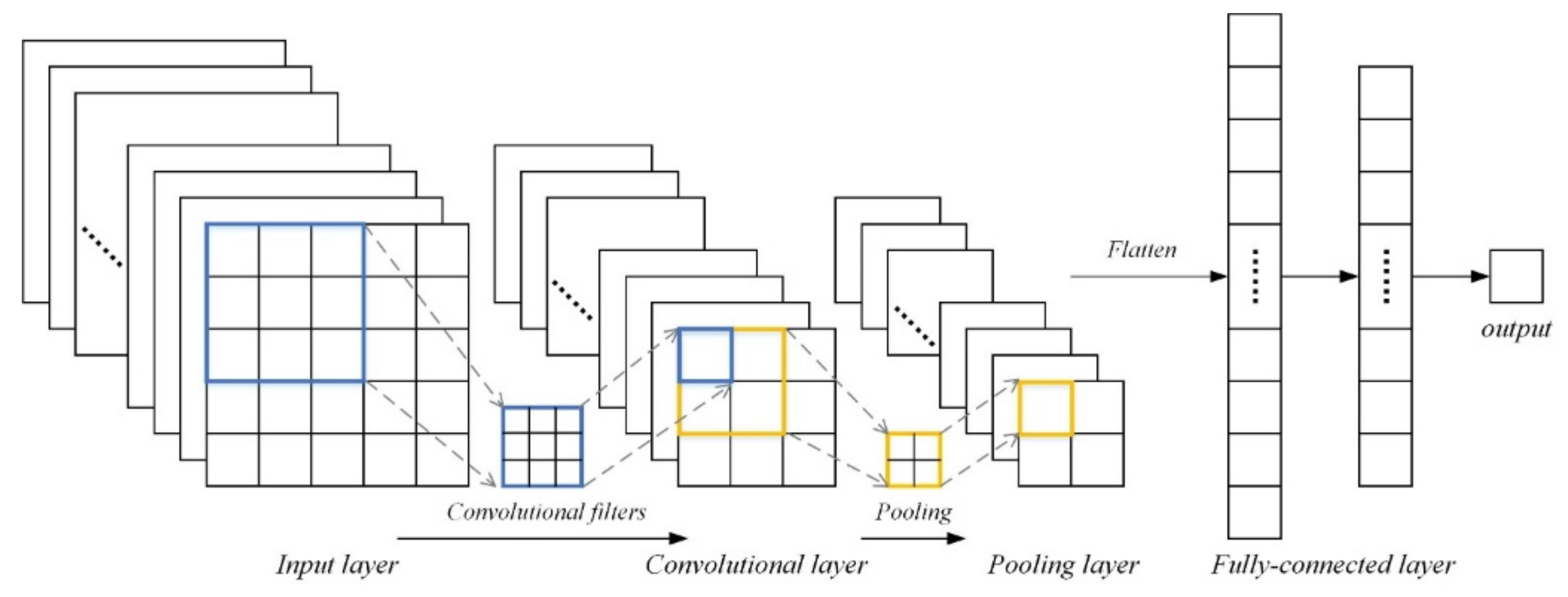
3.1.1. Convolutional Neural Network (CNN) Model

CNN is a deep learning model used mainly to capture spatial features from complex data [35,40]. A traditional CNN model is composed of input layers, hidden layers consisting of convolution layers, pooling layers, fully connected layers, and output layers, as shown in Figure 3.

The CNN model was established by the following steps. First, we converted point data with neighborhood information to an image-like format as the input layers. In particular, each soil sample location pixel was taken as a center, and the center with its neighborhood pixels were taken as the input data. The neighborhood size can be determined by the user. The input data (multiple environmental variables) are shown in Figure 4. The parameters $w$ and $h$ are the width and height of the local image size (window size), $n_c$ is the number of channels, indicating the number of environmental variables, and the center, $p\left(i,j\right)$, is each soil sample location. The window size of the input data of the climate and terrain variables was determined to be 5 × 5 to make the contextual information of the input data consistent with the spatial resolution (500 m) of the phenological variables.

We employed convolutional filtering to extract spatial contextual features for training. The convolution operation used a filter to slide over the input data to obtain the feature maps, and the generated convolution layers were composed of these feature maps. Then, the conventional layers were implemented with a pooling operation. We used the max pooling because it was tested to outperform the other kinds of pooling operations [61]. The pooling operation was employed to decrease the spatial dimension of the convolution layers and the computation cost. The final pooling layer was flattened into a one-dimensional vector to connect with the fully connected layers. The convolution and pooling operations transformed the original input data (multi-environmental variables) into different feature maps containing useful contextual information.

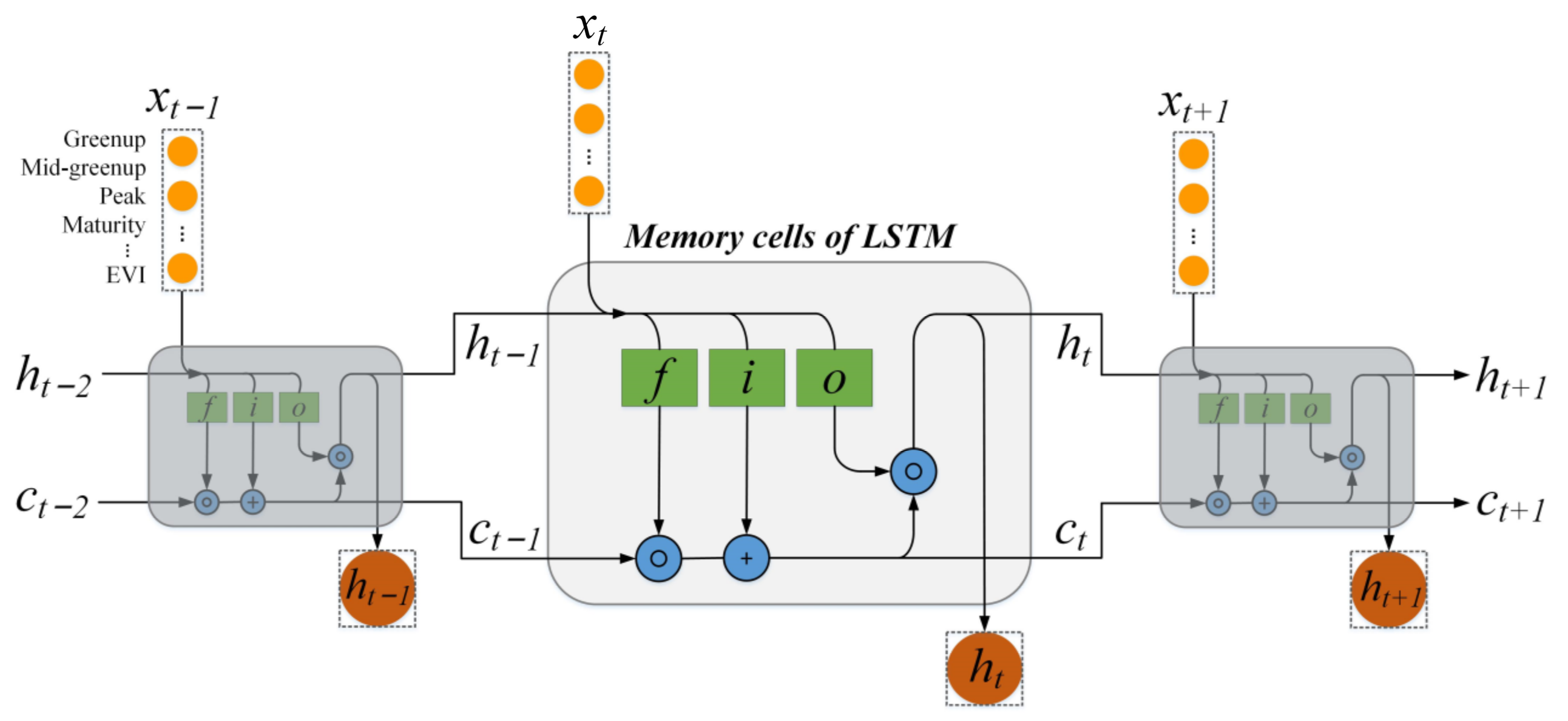
3.1.2. Long Short-Term Memory (LSTM) Model

LSTM is a deep learning model developed for learning temporal features from time-series or sequential data. A typical LSTM model consists of input layers, hidden layers (memory cells), and output layers (Figure 5). The input layer is the time-series data. The hidden layer is composed of one or more memory cells to extract the temporal features of the input data. The cell state ($c$) is a memory of an LSTM cell, which represents the accumulated information from previous time steps. The hidden state ($h$) is an output of a cell. Both of them are controlled by three gates: a forget gate ($f$), an input gate ($i$), and an output gate ($o$) [42,62]. The three gates determine retained information from the previous time step ($t-1$) and how much information to output at the current time step ($t$). In the $t$-th step, the current forget gate ($f_t$) (Equation (2)) of the present memory cell decides how much information from the previous time step should be thrown away before passing into the current cell state ($c_t$). Then, the input gate ($i_t$) (Equation (3)) decides what percentage of information of the potential cell state (${\tilde{c}}_t$) is used to update the current cell state ($c_t$), and $c_t$ is updated by ${\tilde{c}}_t$ and $i_t$ (Equations (4) and (5)). Finally, the output gate ($o_t$) decides what information from the current cell state is provided to the current hidden state ($h_t$), which is regarded as the output from the current memory cell (Equations (6) and (7)).

$$f_t=\sigma \left(W_f{x}_t+U_f{h}_{t-1}+b_f\right)$$

(2)

$$i_t=\sigma \left(W_i{x}_t+U_i{h}_{t-1}+b_i\right)$$

(3)

$${\tilde{c}}_t=tanh\left(W_{\tilde{c}}{x}_t+U_{\tilde{c}}{h}_{t-1}+b_{\tilde{c}}\right)$$

(4)

$$c_t=f_t\times c_{t-1}+i_t\times {\tilde{c}}_t$$

(5)

$$o_t=\sigma \left(W_o{x}_t+U_o{h}_{t-1}+b_o\right)$$

(6)

$$h_t=tanh\left(c_t\right)\times o_t$$

(7)

where $W_f$, $U_f$, $W_{\tilde{c}}$, $U_c$, $W_i$, $U_i$, $W_o$, and $U_o$ are weight matrices; $b_f$, $b_i$, $b_{\tilde{c}}$, and $b_o$ are bias; $x_t$ is the currrent input; $h_{t-1}$ is the previous hidden state; the logistic sigmoid $\sigma \left(x\right)=\frac{1}{1+e^{-x}}$ is used as the gate activation function; and the hyperbolic tangent $tanh\left(x\right)=\frac{e^x-e^{-x}}{e^x+e^{-x}}$ is used as the cell input and output activation.

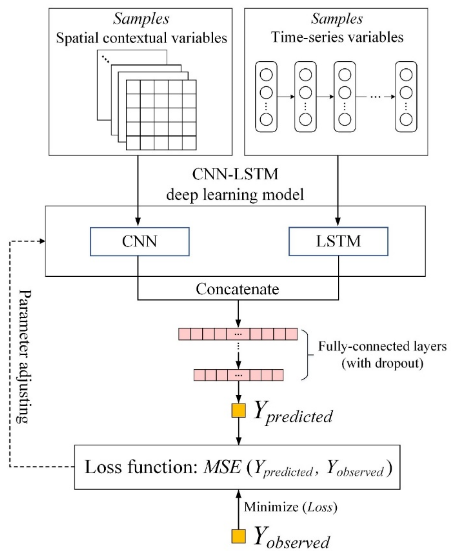
3.1.3. Hybrid Model Architecture of CNN-LSTM

The developed CNN-LSTM model is shown in Figure 6. The basic idea is that the spatial contextual features of climate and terrain are extracted by the CNN model, while the temporal features of the phenology and EVI variables are extracted by the LSTM model. The extracted spatial and temporal features are concatenated to connect the fully connected layers to calculate the outputs (e.g., the predicted SOC).

The calibration of the CNN-LSTM model includes a number of iteration steps for decreasing the error between the predicted values and observed values and adjusting the learnable parameters, such as the weights and biases in the network (Figure 5). The algorithm of back-propagation was applied in the calibration process to adjust the parameters of the network to minimize the overall loss [35]. Because the complex structure of the CNN-LSTM model could increase the risk of over-fitting, we used dropout layers to reduce this negative effect [17,44]. An activation function of ReLU was adopted to implement the nonlinear transformation of the neurons in the network for rapid converging [34].

Some hyperparameters (including the learning rate, the number of neurons, and the depth of the CNN and LSTM networks) needed to be set. There is no fixed method to determine these hyperparameters. The grid search method [63] was used to select appropriate combinations of hyperparameters (

Table 2. Structure of CNN in the CNN-LSTM model.

CNN Layers	Filter Size	Number of Neurons	Activation Function
Convolutional layer	3 × 3	32	ReLU
Max-Pooling layer	2 × 2	-	-
Convolutional layer	3 × 3	64	ReLU
Max-Pooling layer	2 × 2	-	-
Fully connected layer	-	128	ReLU
Output layer	-	1	Linear

and

Table 3. Structure of LSTM in the CNN-LSTM model.

LSTM Layers	Number of Layers	Number of Neurons	Activation Function
Memory cells	2	32	Sigmoid, Tanh

). We selected the minimum mean-square error (MSE) between the observed SOC and the predicted SOC as the loss criterion by using an Adam optimizer. The proposed deep learning model was developed using the PyTorch package [64] in the Python programming language.

3.2. Development of Different Environmental Variable Groups for Models

All environmental variables were divided into four groups (

Table 4. The groups of environmental variables, the numbers of environmental variables, and the models applied for soil organic carbon prediction.

Group Name	The Included Variable Categories	The Number of Variables	Deep Learning Model	Reference Model
Group 1	Climate, terrain	10	CNN	RF
Group 2	Climate, terrain, phenology	120	CNN-LSTM	RF
Group 3	Climate, terrain, EVI	20	CNN-LSTM	RF
Group 4	Climate, terrain, phenology, EVI	130	CNN-LSTM	RF

) to evaluate the performance of different combinations of predictors on SOC prediction with the deep learning models (the CNN model and the CNN-LSTM model) and a reference model, the random forest (RF) model. The first group was composed of commonly used variables, including climate and terrain. The second group was composed of the variables in the first group and the phenological variables. The third group was composed of the variables in the first group and the EVI variables. The fourth group was composed of all four categories of variables. Because of the different types of variables in these groups, we used CNN for the climate and terrain variables, which were treated as static variables, and used CNN-LSTM for the other three groups. The total number of variables in each group for SOC prediction is shown in Table 4. For example, the total number of variables in the fourth group is 130, including 2 climate variables, 8 topographic variables, 110 phenological variables (11 × 10 years), and 10 EVI variables (1 × 10 years).

3.3. Evaluation of SOC Predictions

We applied a five-fold cross-validation to test the soil predictions using combinations of different groups of variables and different models. All soil samples were partitioned into five subsets based on a stratified strategy, with the parent lithology types as strata [15]. Each subset was used for testing the prediction results, and each of the remaining nine subsets was taken as a training set. To select the hyperparameters of the deep learning model, each training set was partitioned into a validation set and a training set, and the optimal hyperparameters were determined according to the model performance on the validation set. The performance of the different models was evaluated by two indices: the root-mean-square error (RMSE) (Equation (9)) and the coefficient of determination (${\mathrm{R}}^2$):

$$\mathrm{RMSE}=\sqrt{\frac{{{\displaystyle \sum }}_{i=1}^n{({\widehat{y}}_i-y_i)}^2}{n}}$$

(8)

$${\mathrm{R}}^2=1-\frac{{{\displaystyle \sum }}_{i=1}^n{\left(y_i-{\widehat{y}}_i\right)}^2}{{{\displaystyle \sum }}_{i=1}^n{\left(y_i-\overline{y}\right)}^2}$$

(9)

where ${\widehat{y}}_i$ and $y_i$ are the prediction and observation of SOC content at $i$-th soil samples, $n$ is the number of soil samples, and $\overline{y}$ is the average of $n$ observed SOC values.

The cross-validation was adopted for the evaluation of model performance. The cross-validated metrics of accuracy can reveal the model stability and prevent bias in evaluation caused by the overfitting of the model to a single validation set. We repeated the five-fold cross-validation ten times to reduce the influence of the randomness of only one data split. The average cross-validation accuracy of the ten times was taken as the final evaluation of model performance.

The RF model was taken as a reference model and was executed using all the groups of environmental variables to be compared with the deep learning models. The biggest advantage of RF is that it is an ensemble model that employs subsets of data for training the base learners and aggregates the predicted results of all base learners [65]. Thus, it can effectively reduce the overfitting risk and achieve a better generalization ability. RF has been tested to be superior to many other machine learning models [30,66,67]. Therefore, taking RF as a baseline model is more challenging for testing the performance of the proposed deep learning model. The RF model was built using the scikit-learn [68] package in Python.

4. Results

4.1. Description of Characteristics of SOC

According to

Table 5. Description of statistical characteristics of soil samples.

Sample Density (10−2 Number/km2)	Minimum (g/kg)	Maximum (g/kg)	Mean (g/kg)	Median (g/kg)	Standard Deviation (g/kg)
5.51	2.53	38.59	12.63	11.49	5.88

, the study area had a large range of SOC content (2.53~38.59 g/kg), with an average of 12.63 g/kg. The sample density in the study area was 5.51 × 10⁻² per km². Most soil samples were located in cultivated land with a gentle topography, and a small number of sampling points were located in forested land, which usually had a large SOC content (Figure 1c).

4.2. Correlation between SOC and Environmental Variables

The correlations between SOC and all environmental covariates are shown in Figure 7. Temperature and precipitation showed highly negative and positive relationships with SOC, respectively. Most topographic variables had high correlations with SOC. The high positive relationship between elevation and SOC reflects that the flat areas with higher intensities of human cultivation were more likely to have less soil carbon.

Among the phenological variables, in most years the evi-minimum, evi-amplitude, and maturity showed the highest correlation with SOC, and the mid-greenup and peak followed. The correlation between evi-mean and SOC was also relatively high in all ten years. The phenological and EVI variables did not have a specific year with an extremely high correlation with SOC.

Generally, the climate and terrain variables were more strongly correlated with SOC compared with the phenological and EVI variables. However, the strongest correlations were almost all under 0.5. Similar low correlations were also found in some previous studies [69,70]. Therefore, there is often a nonlinear relationship between SOC and environmental variables.

4.3. Comparisons of the Predicted Results for Deep Learning and RF

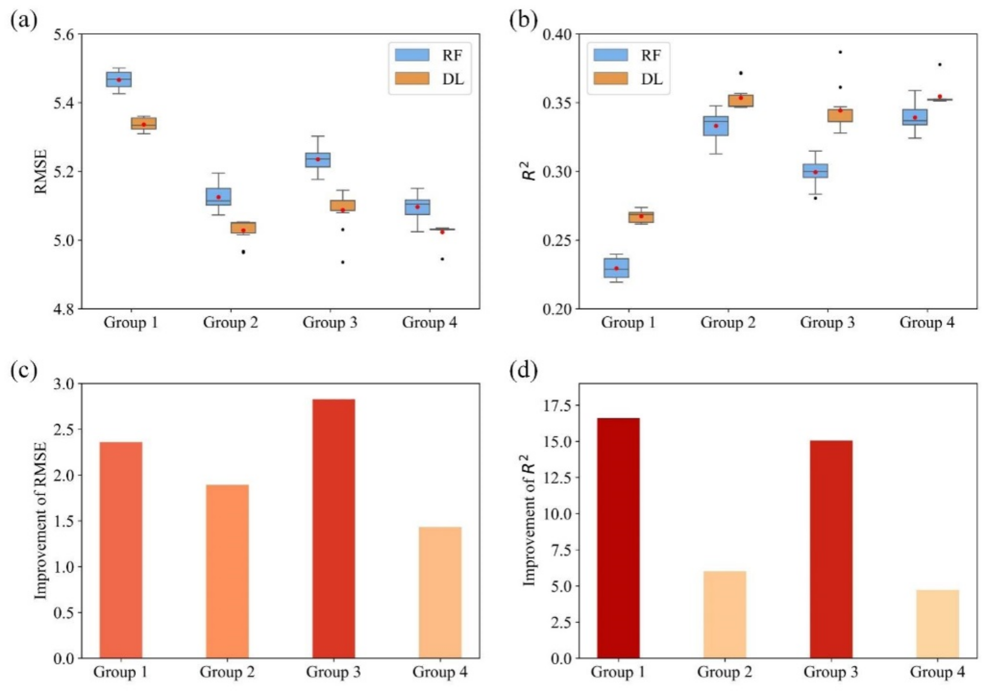
4.3.1. Comparisons of the Prediction Accuracies

The boxplots of RMSE and ${\mathrm{R}}^2$ using the deep learning and RF models based on different environmental groups are shown in Figure 8a,b. In general, the deep learning model generated a higher cross-validation accuracy than RF with each group of covariates. Whether using RF or the deep learning model, adding time series of phenological and/or EVI variables to the climatic and topographic variables improved model performance. This confirmed the important role of temporal vegetation variables in predicting SOC. The general higher accuracies of the deep learning models compared to RF reflects the advantages of deep learning models in considering both spatial contextual information and the temporal variation characteristics of covariates. The accuracy in the second group was higher than that using the third group, which demonstrates that adding phenological variables to the climatic and topographic variables performed better than only adding the EVI variables in our study area. The CNN-LSTM model that was fed all covariates (group 4) was the most accurate model, suggesting the combination of a convolutional neural network and a recurrent neural network is more capable of synthesizing complex spatial and temporal information for processing complex features in space and time. In addition, the variance of the ten repeated cross-validation accuracies using each group of environmental covariates with deep learning was generally smaller than that with RF.

The accuracy improvements of deep learning compared to RF in the four groups of covariates were 2.36%, 1.89%, 2.83%, and 1.43% in terms of RMSE and 16.59%, 6.01%, 15.05%, and 4.72% in terms of ${\mathrm{R}}^2$, respectively (Figure 8c,d). It can be seen that the deep learning models showed a larger improvement in accuracy when using the covariates of group 1 and group 3 without phenological variables. This indicates that adding more informative predictors (multi-year phenological variables) improves RF prediction accuracy more than adding EVI variables. The difference in deep learning accuracy between using groups 2, 3, and 4 was not large. This might result from the powerful learning ability of LSTM that effectively extracts more latent information from long time series vegetation variations when only EVI information is provided, while it is difficult for RF to fully extract temporal variation characteristics by only using the EVI variable.

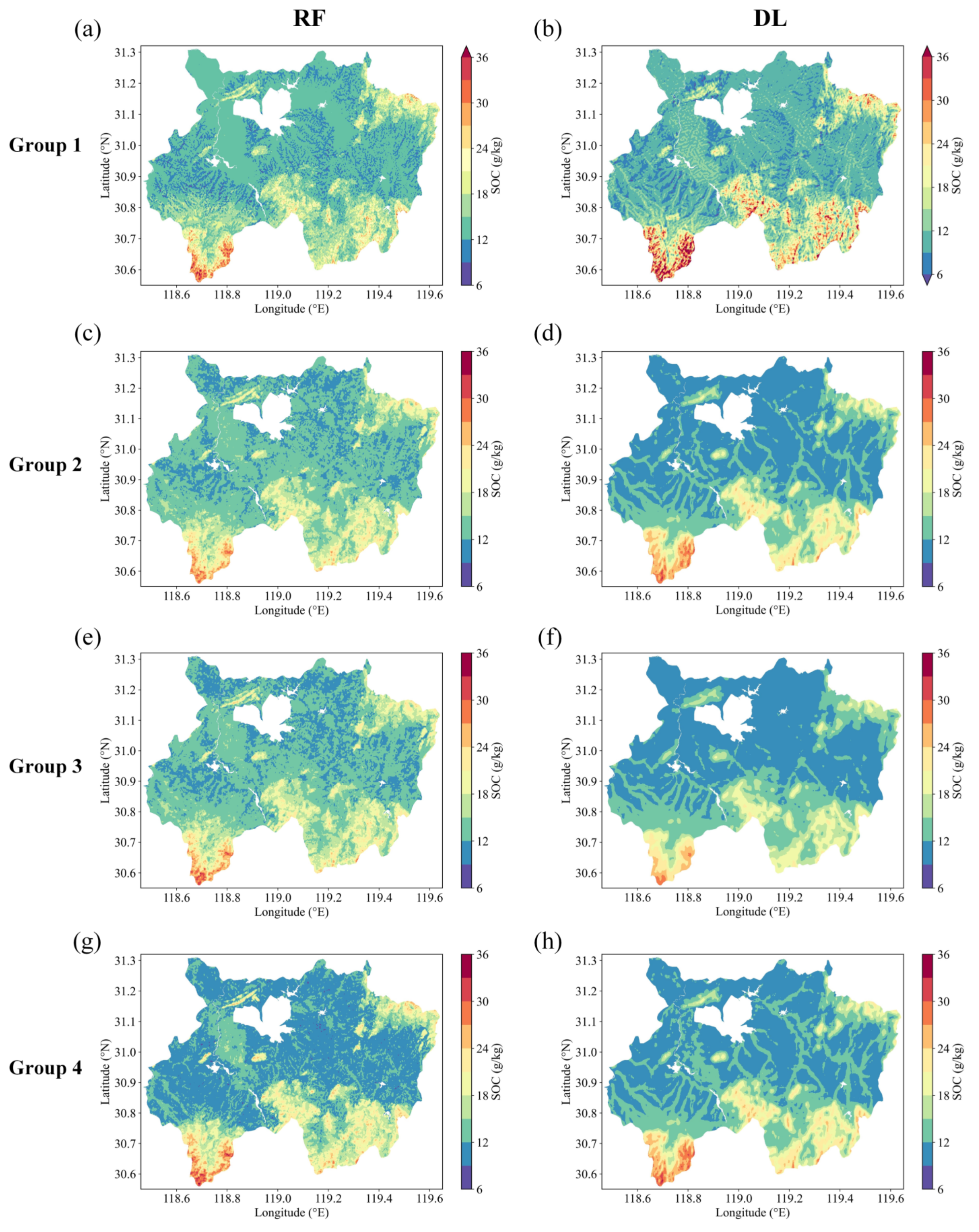
4.3.2. Comparisons of Predicted Maps

The predicted SOC maps based on the fitted RF and deep learning models with four groups of covariates are shown in Figure 9. The spatial distributions of SOC content in all predicted maps showed similar patterns. Generally, the southern and northeast mountain areas, with forest as the main land cover type, had higher SOC while the northern and central areas, with a gentle topography (mainly cultivated land), had lower SOC contents. However, there were some differences between these predicted maps. The maps predicted by using the first group of covariates were more fragmentized than when using the other groups (Figure 9a,b). This may be because of the limited environmental variables, leading to the model to be more inclined to fit the spatial characteristics of terrain factors. In addition, according to the SOC maps generated in previous studies in this area [15,71], the predicted maps based on CNN-LSTM models (group 2–4) showed a more reasonable spatial distribution of SOC than that based on RF models (Figure 9c–h). The maps generated with CNN-LSTM showed a smoother effect, which indicates deep learning is more capable of capturing more general SOC spatial distribution characteristics by extracting spatial contextual information and long time series features. Our results also support that a previous study found that a predicted map generated with CNN was less speckled in appearance because the DL method adopts neighbor pixels for model training [43].

5. Discussion

5.1. Long Time Series of Phenological Variables Used for SOC Prediction

The fourth group of environmental covariates, which included the long time series of EVI and phenological variables for SOC prediction, obtained better performance through deep learning compared with the other groups. This reminds us of the key role of incorporating temporal information of aboveground vegetation for mapping the belowground soil information. We selected a study area that was mainly covered by cultivated land and forest with different phenologies (Figure 1 and Figure 2). Plants strongly interacted with soil, and the phenology could effectively indicate the significant growth stage of the plants compared with the vegetation indices. Therefore, the land surface phenology exhibits a great potential to improve the accuracy of digital soil mapping. So far, few researchers have used short time series of phenological data to predict SOC. For example, one and two years of key phenological dates were used for SOC prediction in [12,16]. Furthermore, over a long period of time, the soil carbon input may be strongly affected by plant growth, which is controlled by phenology. Thus, long time series of phenology may be beneficial for improving the accuracy of predicting SOC; however, this information was seldom used for SOC prediction. The greatest challenge to the use of long-term phenology (such as the ten-year phenological observations used in this study) for SOC prediction is the effective extraction of the temporal features contained in the long time series. The LSTM model is able to solve this challenge since it is specially designed for time-series data. As expected, the better accuracy of the CNN-LSTM model in our study validated that long time series of phenological variables applied with deep learning are helpful for SOC predictions.

The uncertainty of the vegetation information estimated from remote sensing observations is an important issue affecting the accuracy of predictive models [72]. Currently, the Visible Infrared Imaging Radiometer Suite global land surface phenology (VIIRS GLSP) product provides a supplement to the MOCD12Q2 product and has been available since 2013 [73]. This product is able to provide more detailed long time series of phenological variables for soil prediction if the spatial resolution of the MODIS data does not meet the requirement. The spatial resolution (500 m) of the phenological data may be coarse for studies at a finer scale. Downscaling the phenology product can be a possible way to solve the coarse spatial resolution issue, but multi-source remote sensing data fusion could be an acceptable way to generate more detailed phenological variables in the future.

5.2. Applicability of Deep Learning

The CNN-LSTM model has the advantage of extracting features from both the spatial and temporal domains and is capable of processing complex and large environmental input variables. In our study area, the climate, terrain, and the phenological/EVI variables contained spatial contextual and temporal information. Thus, the CNN-LSTM model was more appropriate for simultaneously extracting the spatial and temporal features of different types of environmental variables for SOC prediction. Few previous studies used an approach similar to the CNN-LSTM model for dealing with different types of environmental variables in SOC predictions. With various types of data (e.g., time-series, spatial, and spectral data) becoming available for soil predictions, advanced methods are required, especially for predicting soil dynamics. The developed CNN-LSTM model would be a promising technique for soil predictions and handling a large number of environmental variables.

The window size used in the CNN model influenced the accuracy of soil prediction. In our study, the window sizes of the climatic and topographic variables were selected as 5 × 5 (450 m), which was close to the spatial resolution of the phenological variables. To simply the model structure, using different variables under the same window size can be adopted. For example, Yang et al. (2021) chose the same window size for different variables [17]. However, we should further consider the window size issue. According to previous studies [44], the window size corresponds to the scale at which the local environment influences soil development, and different regions may need different window sizes. Soil is complex and is influenced by numerous environmental factors, which may act at different local scales (the different spatial size of contextual information). Thus, the window sizes for taking into account the contextual information of different environmental variables for SOC prediction may be different and should be explored in the future.

Deep learning usually requires a large amount of data for model training. Increasing the number of predictors (the environmental covariates in our study) also requires sufficient samples for learning features from predictors. However, in DSM, soil sample data are usually limited due to the high cost of field sampling. In our study, while the performance of CNN-LSTM with the fourth group (130 variables) was the best for SOC mapping, the model accuracy still did not reach an ideal level. The main reason for this might be the limited sample size leading to the inability to explore the internal characteristics of a large number of predictors. Flipping, rotating, scaling, and cropping [34] are common data augmentation methods used for image data. These methods can be used to synchronously augment sample data in the future. Moreover, as soil samples are always insufficient, the existing pedological knowledge related to the soil organic carbon prediction could be incorporated into the DSM framework, thereby reducing the heavy reliance of the predictive model on sample size.

6. Conclusions

In this study, a CNN-LSTM model was developed for predicting SOC in our study area with different groups of environmental covariates. Using spatial features extracted by CNN and temporal features extracted by LSTM effectively improved the accuracy of SOC prediction compared with RF. Adding phenological information of vegetation to the commonly used climate and terrain variables can improve the soil prediction accuracy. Our findings suggest that long time series of land surface phenology can potentially be used for DSM. We conclude that the fine-tuned CNN-LSTM model is an effective alternative model that is even more accurate than the RF model and therefore can be a powerful model for SOC predictive mapping aided by large amounts of environmental covariates with the contextual information in space and time.

References

1. Post, W.M.; Emanuel, W.R.; Zinke, P.J.; Stangenberger, A.G. Soil Carbon Pools and World Life Zones. Nature 1982, 298, 156–159. [Google Scholar] [CrossRef]
2. Batjes, N.H. Total Carbon and Nitrogen in the Soils of the World. Eur. J. Soil Sci. 1996, 47, 151–163. [Google Scholar] [CrossRef]
3. Wang, M.; Xu, S.; Zhao, Y.; Shi, X. Climatic Effect on Soil Organic Carbon Variability as a Function of Spatial Scale. Arch. Agron. Soil Sci. 2017, 63, 375–387. [Google Scholar] [CrossRef]
4. Zhao, Y.; Wang, M.; Hu, S.; Zhang, X.; Ouyang, Z.; Zhang, G.; Huang, B.; Zhao, S.; Wu, J.; Xie, D.; et al. Economics- and Policy-Driven Organic Carbon Input Enhancement Dominates Soil Organic Carbon Accumulation in Chinese Croplands. Proc. Natl. Acad. Sci. USA 2018, 115, 4045–4050. [Google Scholar] [CrossRef]
5. Minasny, B.; Malone, B.P.; McBratney, A.B.; Angers, D.A.; Arrouays, D.; Chambers, A.; Chaplot, V.; Chen, Z.-S.; Cheng, K.; Das, B.S.; et al. Soil Carbon 4 per Mille. Geoderma 2017, 292, 59–86. [Google Scholar] [CrossRef]
6. Yang, L.; Shen, F.; Zhang, L.; Cai, Y.; Yi, F.; Zhou, C. Quantifying Influences of Natural and Anthropogenic Factors on Vegetation Changes Using Structural Equation Modeling: A Case Study in Jiangsu Province, China. J. Clean. Prod. 2021, 280, 124330. [Google Scholar] [CrossRef]
7. Amundson, R.; Berhe, A.A.; Hopmans, J.W.; Olson, C.; Sztein, A.E.; Sparks, D.L. Soil and Human Security in the 21st Century. Science 2015, 348, 1261071. [Google Scholar] [CrossRef] [PubMed]
8. Lal, R. Soil Carbon Sequestration to Mitigate Climate Change. Geoderma 2004, 123, 1–22. [Google Scholar] [CrossRef]
9. Sanchez, P.A.; Ahamed, S.; Carré, F.; Hartemink, A.E.; Hempel, J.; Huising, J.; Lagacherie, P.; McBratney, A.B.; McKenzie, N.J.; Mendonça-Santos, M.d.L.; et al. Digital Soil Map of the World. Science 2009, 325, 680–681. [Google Scholar] [CrossRef]
10. McBratney, A.B.; Mendonça Santos, M.L.; Minasny, B. On Digital Soil Mapping. Geoderma 2003, 117, 3–52. [Google Scholar] [CrossRef]
11. Minasny, B.; McBratney, A.B. Digital Soil Mapping: A Brief History and Some Lessons. Geoderma 2016, 264, 301–311. [Google Scholar] [CrossRef]
12. Yang, L.; Song, M.; Zhu, A.-X.; Qin, C.; Zhou, C.; Qi, F.; Li, X.; Chen, Z.; Gao, B. Predicting Soil Organic Carbon Content in Croplands Using Crop Rotation and Fourier Transform Decomposed Variables. Geoderma 2019, 340, 289–302. [Google Scholar] [CrossRef]
13. Schillaci, C.; Lombardo, L.; Saia, S.; Fantappiè, M.; Märker, M.; Acutis, M. Modelling the Topsoil Carbon Stock of Agricultural Lands with the Stochastic Gradient Treeboost in a Semi-Arid Mediterranean Region. Geoderma 2017, 286, 35–45. [Google Scholar] [CrossRef]
14. Hong, S.; Yin, G.; Piao, S.; Dybzinski, R.; Cong, N.; Li, X.; Wang, K.; Peñuelas, J.; Zeng, H.; Chen, A. Divergent Responses of Soil Organic Carbon to Afforestation. Nat. Sustain. 2020, 3, 694–700. [Google Scholar] [CrossRef]
15. Zhang, L.; Yang, L.; Cai, Y.; Huang, H.; Shi, J.; Zhou, C. A Multiple Soil Properties Oriented Representative Sampling Strategy for Digital Soil Mapping. Geoderma 2022, 406, 115531. [Google Scholar] [CrossRef]
16. Yang, L.; He, X.; Shen, F.; Zhou, C.; Zhu, A.-X.; Gao, B.; Chen, Z.; Li, M. Improving Prediction of Soil Organic Carbon Content in Croplands Using Phenological Parameters Extracted from NDVI Time Series Data. Soil Tillage Res. 2020, 196, 104465. [Google Scholar] [CrossRef]
17. Yang, L.; Cai, Y.; Zhang, L.; Guo, M.; Li, A.; Zhou, C. A Deep Learning Method to Predict Soil Organic Carbon Content at a Regional Scale Using Satellite-Based Phenology Variables. Int. J. Appl. Earth Obs. Geoinf. 2021, 102, 102428. [Google Scholar] [CrossRef]
18. Heuvelink, G.B.M.; Angelini, M.E.; Poggio, L.; Bai, Z.; Batjes, N.H.; van den Bosch, R.; Bossio, D.; Estella, S.; Lehmann, J.; Olmedo, G.F.; et al. Machine Learning in Space and Time for Modelling Soil Organic Carbon Change. Eur. J. Soil Sci. 2021, 72, 1607–1623. [Google Scholar] [CrossRef]
19. Van der Putten, W.H.; Bardgett, R.D.; Bever, J.D.; Bezemer, T.M.; Casper, B.B.; Fukami, T.; Kardol, P.; Klironomos, J.N.; Kulmatiski, A.; Schweitzer, J.A.; et al. Plant–Soil Feedbacks: The Past, the Present and Future Challenges. J. Ecol. 2013, 101, 265–276. [Google Scholar] [CrossRef]
20. Wilson, B.R.; Lonergan, V.E. Land-Use and Historical Management Effects on Soil Organic Carbon in Grazing Systems on the Northern Tablelands of New South Wales. Soil Res. 2013, 51, 668–679. [Google Scholar] [CrossRef]
21. Melillo, J.M.; Frey, S.D.; DeAngelis, K.M.; Werner, W.J.; Bernard, M.J.; Bowles, F.P.; Pold, G.; Knorr, M.A.; Grandy, A.S. Long-Term Pattern and Magnitude of Soil Carbon Feedback to the Climate System in a Warming World. Science 2017, 358, 101–105. [Google Scholar] [CrossRef]
22. Caparros-Santiago, J.A.; Rodriguez-Galiano, V.; Dash, J. Land Surface Phenology as Indicator of Global Terrestrial Ecosystem Dynamics: A Systematic Review. ISPRS J. Photogramm. Remote Sens. 2021, 171, 330–347. [Google Scholar] [CrossRef]
23. Piao, S.; Liu, Q.; Chen, A.; Janssens, I.A.; Fu, Y.; Dai, J.; Liu, L.; Lian, X.; Shen, M.; Zhu, X. Plant Phenology and Global Climate Change: Current Progresses and Challenges. Glob. Change Biol. 2019, 25, 1922–1940. [Google Scholar] [CrossRef] [PubMed]
24. He, X.; Yang, L.; Li, A.; Zhang, L.; Shen, F.; Cai, Y.; Zhou, C. Soil Organic Carbon Prediction Using Phenological Parameters and Remote Sensing Variables Generated from Sentinel-2 Images. CATENA 2021, 205, 105442. [Google Scholar] [CrossRef]
25. Kariyeva, J.; Van Leeuwen, W.J.D. Environmental Drivers of NDVI-Based Vegetation Phenology in Central Asia. Remote Sens. 2011, 3, 203–246. [Google Scholar] [CrossRef]
26. White, M.A.; Running, S.W.; Thornton, P.E. The Impact of Growing-Season Length Variability on Carbon Assimilation and Evapotranspiration over 88 Years in the Eastern US Deciduous Forest. Int. J. Biometeorol. 1999, 42, 139–145. [Google Scholar] [CrossRef] [PubMed]
27. Lange, M.; Eisenhauer, N.; Sierra, C.A.; Bessler, H.; Engels, C.; Griffiths, R.I.; Mellado-Vázquez, P.G.; Malik, A.A.; Roy, J.; Scheu, S.; et al. Plant Diversity Increases Soil Microbial Activity and Soil Carbon Storage. Nat. Commun. 2015, 6, 6707. [Google Scholar] [CrossRef] [PubMed]
28. Piao, S.; Ciais, P.; Friedlingstein, P.; Peylin, P.; Reichstein, M.; Luyssaert, S.; Margolis, H.; Fang, J.; Barr, A.; Chen, A.; et al. Net Carbon Dioxide Losses of Northern Ecosystems in Response to Autumn Warming. Nature 2008, 451, 49–52. [Google Scholar] [CrossRef]
29. Richardson, A.D.; Black, T.A.; Ciais, P.; Delbart, N.; Friedl, M.A.; Gobron, N.; Hollinger, D.Y.; Kutsch, W.L.; Longdoz, B.; Luyssaert, S.; et al. Influence of Spring and Autumn Phenological Transitions on Forest Ecosystem Productivity. Phil. Trans. R. Soc. B 2010, 365, 3227–3246. [Google Scholar] [CrossRef]
30. Zhang, L.; Yang, L.; Ma, T.; Shen, F.; Cai, Y.; Zhou, C. A Self-Training Semi-Supervised Machine Learning Method for Predictive Mapping of Soil Classes with Limited Sample Data. Geoderma 2021, 384, 114809. [Google Scholar] [CrossRef]
31. Maynard, J.J.; Levi, M.R. Hyper-Temporal Remote Sensing for Digital Soil Mapping: Characterizing Soil-Vegetation Response to Climatic Variability. Geoderma 2017, 285, 94–109. [Google Scholar] [CrossRef]
32. Were, K.; Bui, D.T.; Dick, Ø.B.; Singh, B.R. A Comparative Assessment of Support Vector Regression, Artificial Neural Networks, and Random Forests for Predicting and Mapping Soil Organic Carbon Stocks across an Afromontane Landscape. Ecol. Indic. 2015, 52, 394–403. [Google Scholar] [CrossRef]
33. Hengl, T.; Heuvelink, G.B.M.; Stein, A. A Generic Framework for Spatial Prediction of Soil Variables Based on Regression-Kriging. Geoderma 2004, 120, 75–93. [Google Scholar] [CrossRef]
34. Krizhevsky, A.; Sutskever, I.; Hinton, G.E. ImageNet Classification with Deep Convolutional Neural Networks. Commun. ACM 2017, 60, 84–90. [Google Scholar] [CrossRef]
35. LeCun, Y.; Bengio, Y.; Hinton, G. Deep Learning. Nature 2015, 521, 436–444. [Google Scholar] [CrossRef]
36. Behrens, T.; Schmidt, K.; MacMillan, R.A.; Rossel, R.A.V. Multi-Scale Digital Soil Mapping with Deep Learning. Sci. Rep. 2018, 8, 15244. [Google Scholar] [CrossRef]
37. Yuan, Q.; Shen, H.; Li, T.; Li, Z.; Li, S.; Jiang, Y.; Xu, H.; Tan, W.; Yang, Q.; Wang, J.; et al. Deep Learning in Environmental Remote Sensing: Achievements and Challenges. Remote Sens. Environ. 2020, 241, 111716. [Google Scholar] [CrossRef]
38. Zhang, L.; Na, J.; Zhu, J.; Shi, Z.; Zou, C.; Yang, L. Spatiotemporal Causal Convolutional Network for Forecasting Hourly PM2.5 Concentrations in Beijing, China. Comput. Geosci. 2021, 155, 104869. [Google Scholar] [CrossRef]
39. James, T.; Schillaci, C.; Lipani, A. Convolutional Neural Networks for Water Segmentation Using Sentinel-2 Red, Green, Blue (RGB) Composites and Derived Spectral Indices. Int. J. Remote Sens. 2021, 42, 5338–5365. [Google Scholar] [CrossRef]
40. Reichstein, M.; Camps-Valls, G.; Stevens, B.; Jung, M.; Denzler, J.; Carvalhais, N.; Prabhat. Deep Learning and Process Understanding for Data-Driven Earth System Science. Nature 2019, 566, 195–204. [Google Scholar] [CrossRef]
41. Lecun, Y.; Bottou, L.; Bengio, Y.; Haffner, P. Gradient-Based Learning Applied to Document Recognition. Proc. IEEE 1998, 86, 2278–2324. [Google Scholar] [CrossRef]
42. Hochreiter, S.; Schmidhuber, J. Long Short-Term Memory. Neural Comput. 1997, 9, 1735–1780. [Google Scholar] [CrossRef]
43. Padarian, J.; Minasny, B.; McBratney, A.B. Using Deep Learning for Digital Soil Mapping. SOIL 2019, 5, 79–89. [Google Scholar] [CrossRef]
44. Wadoux, A.M.J.C. Using Deep Learning for Multivariate Mapping of Soil with Quantified Uncertainty. Geoderma 2019, 351, 59–70. [Google Scholar] [CrossRef]
45. Singh, S.; Kasana, S.S. Estimation of Soil Properties from the EU Spectral Library Using Long Short-Term Memory Networks. Geoderma Reg. 2019, 18, e00233. [Google Scholar] [CrossRef]
46. Singh, S.; Kasana, S.S. Quantitative Estimation of Soil Properties Using Hybrid Features and RNN Variants. Chemosphere 2022, 287, 131889. [Google Scholar] [CrossRef]
47. Fang, K.; Shen, C.; Kifer, D.; Yang, X. Prolongation of SMAP to Spatiotemporally Seamless Coverage of Continental U.S. Using a Deep Learning Neural Network. Geophys. Res. Lett. 2017, 44, 11030–11039. [Google Scholar] [CrossRef]
48. Li, Q.; Zhu, Y.; Shangguan, W.; Wang, X.; Li, L.; Yu, F. An Attention-Aware LSTM Model for Soil Moisture and Soil Temperature Prediction. Geoderma 2022, 409, 115651. [Google Scholar] [CrossRef]
49. Yang, L.; Li, X.; Yang, Q.; Zhang, L.; Zhang, S.; Wu, S.; Zhou, C. Extracting Knowledge from Legacy Maps to Delineate Eco-Geographical Regions. Int. J. Geogr. Inf. Sci. 2021, 35, 250–272. [Google Scholar] [CrossRef]
50. Yang, L.; Zhu, A.-X.; Zhao, Y.; Li, D.; Zhang, G.; Zhang, S.; Band, L.E. Regional Soil Mapping Using Multi-Grade Representative Sampling and a Fuzzy Membership-Based Mapping Approach. Pedosphere 2017, 27, 344–357. [Google Scholar] [CrossRef]
51. Nelson, D.W.; Sommers, L.E. Total Carbon, Organic Carbon, and Organic Matter. In Methods of Soil Analysis; John Wiley & Sons, Ltd.: Hoboken, NJ, USA, 1996; pp. 961–1010. [Google Scholar]
52. Fick, S.E.; Hijmans, R.J. WorldClim 2: New 1-Km Spatial Resolution Climate Surfaces for Global Land Areas. Int. J. Climatol. 2017, 37, 4302–4315. [Google Scholar] [CrossRef]
53. Amatulli, G.; McInerney, D.; Sethi, T.; Strobl, P.; Domisch, S. Geomorpho90m, Empirical Evaluation and Accuracy Assessment of Global High-Resolution Geomorphometric Layers. Sci. Data 2020, 7, 162. [Google Scholar] [CrossRef]
54. Ganguly, S.; Friedl, M.A.; Tan, B.; Zhang, X.; Verma, M. Land Surface Phenology from MODIS: Characterization of the Collection 5 Global Land Cover Dynamics Product. Remote Sens. Environ. 2010, 114, 1805–1816. [Google Scholar] [CrossRef]
55. Moon, M.; Zhang, X.; Henebry, G.M.; Liu, L.; Gray, J.M.; Melaas, E.K.; Friedl, M.A. Long-Term Continuity in Land Surface Phenology Measurements: A Comparative Assessment of the MODIS Land Cover Dynamics and VIIRS Land Surface Phenology Products. Remote Sens. Environ. 2019, 226, 74–92. [Google Scholar] [CrossRef]
56. Zhang, X.; Friedl, M.A.; Schaaf, C.B.; Strahler, A.H.; Hodges, J.C.F.; Gao, F.; Reed, B.C.; Huete, A. Monitoring Vegetation Phenology Using MODIS. Remote Sens. Environ. 2003, 84, 471–475. [Google Scholar] [CrossRef]
57. Huete, A.; Didan, K.; Miura, T.; Rodriguez, E.P.; Gao, X.; Ferreira, L.G. Overview of the Radiometric and Biophysical Performance of the MODIS Vegetation Indices. Remote Sens. Environ. 2002, 83, 195–213. [Google Scholar] [CrossRef]
58. Huete, A.R.; Liu, H.Q.; Batchily, K.; van Leeuwen, W. A Comparison of Vegetation Indices over a Global Set of TM Images for EOS-MODIS. Remote Sens. Environ. 1997, 59, 440–451. [Google Scholar] [CrossRef]
59. Hengl, T.; de Jesus, J.M.; Heuvelink, G.B.M.; Gonzalez, M.R.; Kilibarda, M.; Blagotić, A.; Shangguan, W.; Wright, M.N.; Geng, X.; Bauer-Marschallinger, B.; et al. SoilGrids250m: Global Gridded Soil Information Based on Machine Learning. PLoS ONE 2017, 12, e0169748. [Google Scholar] [CrossRef]
60. Poggio, L.; de Sousa, L.M.; Batjes, N.H.; Heuvelink, G.B.M.; Kempen, B.; Ribeiro, E.; Rossiter, D. SoilGrids 2.0: Producing Soil Information for the Globe with Quantified Spatial Uncertainty. SOIL 2021, 7, 217–240. [Google Scholar] [CrossRef]
61. Scherer, D.; Müller, A.; Behnke, S. Evaluation of Pooling Operations in Convolutional Architectures for Object Recognition. In Proceedings of the Artificial Neural Networks—ICANN 2010; Diamantaras, K., Duch, W., Iliadis, L.S., Eds.; Springer: Berlin/Heidelberg, Germany, 2010; pp. 92–101. [Google Scholar]
62. Van Houdt, G.; Mosquera, C.; Nápoles, G. A Review on the Long Short-Term Memory Model. Artif. Intell. Rev. 2020, 53, 5929–5955. [Google Scholar] [CrossRef]
63. Lee, W.-Y.; Park, S.-M.; Sim, K.-B. Optimal Hyperparameter Tuning of Convolutional Neural Networks Based on the Parameter-Setting-Free Harmony Search Algorithm. Optik 2018, 172, 359–367. [Google Scholar] [CrossRef]
64. Paszke, A.; Gross, S.; Massa, F.; Lerer, A.; Bradbury, J.; Chanan, G.; Killeen, T.; Lin, Z.; Gimelshein, N.; Antiga, L.; et al. PyTorch: An Imperative Style, High-Performance Deep Learning Library. In Proceedings of the Advances in Neural Information Processing Systems, Vancouver, BC, Canada, 8–14 December 2019; Curran Associates, Inc.: Sydney, Australia, 2019; Volume 32. [Google Scholar]
65. Breiman, L. Random Forests. Mach. Learn. 2001, 45, 5–32. [Google Scholar] [CrossRef]
66. Brungard, C.W.; Boettinger, J.L.; Duniway, M.C.; Wills, S.A.; Edwards, T.C. Machine Learning for Predicting Soil Classes in Three Semi-Arid Landscapes. Geoderma 2015, 239, 68–83. [Google Scholar] [CrossRef]
67. Heung, B.; Ho, H.C.; Zhang, J.; Knudby, A.; Bulmer, C.E.; Schmidt, M.G. An Overview and Comparison of Machine-Learning Techniques for Classification Purposes in Digital Soil Mapping. Geoderma 2016, 265, 62–77. [Google Scholar] [CrossRef]
68. Pedregosa, F.; Varoquaux, G.; Gramfort, A.; Michel, V.; Thirion, B.; Grisel, O.; Blondel, M.; Prettenhofer, P.; Weiss, R.; Dubourg, V.; et al. Scikit-Learn: Machine Learning in Python. J. Mach. Learn. Res. 2011, 12, 2825–2830. [Google Scholar]
69. Goydaragh, M.G.; Taghizadeh-Mehrjardi, R.; Jafarzadeh, A.A.; Triantafilis, J.; Lado, M. Using Environmental Variables and Fourier Transform Infrared Spectroscopy to Predict Soil Organic Carbon. CATENA 2021, 202, 105280. [Google Scholar] [CrossRef]
70. Li, X.; Shang, B.; Wang, D.; Wang, Z.; Wen, X.; Kang, Y. Mapping Soil Organic Carbon and Total Nitrogen in Croplands of the Corn Belt of Northeast China Based on Geographically Weighted Regression Kriging Model. Comput. Geosci. 2020, 135, 104392. [Google Scholar] [CrossRef]
71. Zeng, C.; Yang, L.; Zhu, A.-X.; Rossiter, D.G.; Liu, J.; Liu, J.; Qin, C.; Wang, D. Mapping Soil Organic Matter Concentration at Different Scales Using a Mixed Geographically Weighted Regression Method. Geoderma 2016, 281, 69–82. [Google Scholar] [CrossRef]
72. Minasny, B.; Arrouays, D.; Cardinael, R.; Chabbi, A.; Farrell, M.; Henry, B.; Koutika, L.-S.; Ladha, J.K.; McBratney, A.; Padarian, J.; et al. Current NPP Cannot Predict Future Soil Organic Carbon Sequestration Potential. Comment on “Photosynthetic Limits on Carbon Sequestration in Croplands”. Geoderma 2022, 424, 115975. [Google Scholar] [CrossRef]
73. Zhang, X.; Jayavelu, S.; Liu, L.; Friedl, M.A.; Henebry, G.M.; Liu, Y.; Schaaf, C.B.; Richardson, A.D.; Gray, J. Evaluation of Land Surface Phenology from VIIRS Data Using Time Series of PhenoCam Imagery. Agric. For. Meteorol. 2018, 256–257, 137–149. [Google Scholar] [CrossRef]
Figure 1. The location (a), elevation (b), and soil sample locations overlaid on the land cover map (c) of the study area.
Remotesensing 14 04441 g001
Figure 2. Maps of averaged values of phenological variables from 2002 to 2011 extracted from the land cover dynamics product (MCD12Q2) for the study area.
Remotesensing 14 04441 g002
Figure 3. An example of the structure of a convolutional neural network (CNN) model.
Remotesensing 14 04441 g003
Figure 4. The contextual spatial information of climate and topographic covariates as the input supplied to the convolutional neural network (CNN) model.
Remotesensing 14 04441 g004
Figure 5. The architecture of a typical LSTM model. X t 1 , X t , and X t + 1 represent the inputs from time t 1 to time t + 1 ; h t 2 , h t 1 , h t , and h t + 1 represent the outputs; c t 2 , c t 1 , c t , and c t + 1 represent the cell states; f is the forget gate; i is the input gate; and o is the output gate.
Remotesensing 14 04441 g005
Figure 6. The calibration of the CNN-LSTM model of one iteration step with sample data. The model adjusts its parameters by minimizing the mean-square error (MSE) between the observed and predicted target variables.
Remotesensing 14 04441 g006
Figure 7. Correlations of soil organic carbon (SOC) content in the year of 2011 with environmental variables in the study area. (a) Correlations with climatic and topographic variables; (b) correlations with historical phenological and vegetation index variables from 2002 to 2011. The meanings of the abbreviations of all variables can be found in Table 1.
Remotesensing 14 04441 g007
Figure 8. Accuracy and accuracy improvement in terms of RMSE (a,c) and R2 (b,d) for predicting SOC using the four groups of covariates with the deep learning (DL) and random forest (RF) models. Note: For the DL models, the CNN model was adopted for the first group, and the CNN-LSTM model was adopted for other three groups.
Remotesensing 14 04441 g008
Figure 9. The predicted maps of soil organic carbon content (SOC) based on the deep learning (DL) (a,c,e,g) and random forest (RF) (b,d,f,h) models (shown in two columns) with four groups of covariates (shown in four rows).
Remotesensing 14 04441 g009