Article

Proximal Soil Sensing of Low Salinity in Southern Xinjiang, China

1
College of Agriculture, Tarim University, Alar 843300, China
2
Key Laboratory for Geographical Process Analysis & Simulation of Hubei Province, College of Urban & Environmental Sciences, Central China Normal University, Wuhan 430079, China
3
Soils & Water Use Department, Agricultural & Biological Research Institute, National Research Centre, Cairo 12622, Egypt
4
Department of Land Resource Management, School of Tourism and Urban Management, Jiangxi University of Finance and Economics, Nanchang 330000, China
*
Author to whom correspondence should be addressed.
Remote Sens. 2022, 14(18), 4448; https://doi.org/10.3390/rs14184448
Submission received: 12 July 2022 / Revised: 2 September 2022 / Accepted: 3 September 2022 / Published: 6 September 2022
(This article belongs to the Special Issue Remote Sensing of Soil Salinity: Detection and Quantification)

Abstract

:
Measuring the soil salinity using visible and near-infrared (vis–NIR) reflectance spectra is considered a fast and cost-effective method. For monitoring purposes, estimating soils with low salinity measured as electrical conductivity (EC) using vis–NIR spectra is still understudied. In this research, 399 legacy soil samples from six regions of Southern Xinjiang, China with low EC values were used. Reflectance spectra were measured in the laboratory on dried and ground soil samples using a portable vis–NIR spectrometer. By using 10-fold cross-validation, three algorithms–partial least-squares regression (PLSR), random forest (RF), and Cubist–were employed to develop statistical models of EC. The model performance evaluation was obtained by the relative importance of variants. In terms of accuracy assessment of soil EC prediction, the results demonstrated that the Cubist model performed better ( R 2 = 0.67, RMSE = 0.16 mS/cm, RPIQ = 2.28) than both PLSR and RF. Despite similar variants for modelling, the RF model performed somewhat better than that of the PLSR. Additionally, the 610 nm and 790 nm wavelengths only demonstrated significant promise for predicting low soil EC values when used in the Cubist mode. The current research recommends the use of Cubist to estimate the low soil salinity using the vis–NIR reflectance spectra.

Graphical Abstract

1. Introduction

During the last several decades, technological advances have prompted researchers to look into the use of remote or proximal, or both types of sensors to acquire information about soil salinity more rapidly and efficiently. Remote sensing enables soil salinity mapping more regularly and across large areas [1,2,3]. The method does not require intensive access to the field, but due to interference from the environment, such as vegetation cover and soil moisture, it is challenging to obtain pure spectral information of saline soils [4].
The development of proximal soil sensing utilizing electromagnetic induction (EMI) was prompted by the need for simple, trustworthy, and quick measurements of soil salinity gathered at field and landscape scales. This technology allows vast regions to be covered in a short amount of time with either manual determination in the field or an on-the-go system [5,6,7]. These devices measure the apparent electrical conductivity (ECa) of the soil, which is frequently used as a proxy for soil salinity. Nevertheless, the drift and erroneous readings are considered one of the disadvantages during the measurements and are caused by incorrect settings on the Quad and Initial phases [8]. In addition to land cover and topography, factors such as air temperature and weather conditions could affect the in situ measurements [9].
Over the last few decades, many reports have demonstrated that modern spectroscopy in the visible (vis, from 400 to 700 nm) and near-infrared (NIR, from 700 to 2500 nm) regions can determine the EC in soil [10]. Unlike the traditional approaches, measurements with a portable vis–NIR spectrometer could take place under various soil moisture conditions ranging from dried ground to wet soils. Moreover, algorithms such as external parameter orthogonalization (EPO, [11]) or direct standardisation (DS, [12]), make it possible to eliminate the effects of soil moisture on vis–NIR spectra in the field. Measurements in the vis–NIR spectroscopic range are considered to be quick and economical, and have been demonstrated to be practically accurate enough [13]. Therefore, they might be considered as an alternative to conventional laboratory analysis. The primary causes of this include internal vibrational modes of carbonate, neutral water molecules, and hydroxyl groups, which are generally attributable to the distinctive wavelengths of minerals in the range of 400 to 2500 nm [1].
Quantifying soil properties (e.g., salinity) with spectra requires calibration between the complex spectral absorption patterns and the target analytical soil data to derive a spectroscopic model [14]. As a result, the selection of the calibration method can be a crucial factor in the accuracy of soil properties estimations utilising the spectra technique. Over the past ten years, linear regression models such as the partial least-squares regression and stepwise multiple linear regression have gained popularity. The application of machine learning techniques, such as support vector machines, random forests, Cubist and artificial neural networks, to improve estimation accuracy, has recently been the most popular trend in the soil spectrum model [15,16,17,18].
Despite the large and promising literature on soil salinity prediction using vis–NIR spectra, the majority of the estimation has concentrated on saline soils or soils with medium to high value of EC. There is a critical necessity for timely detection and early warning of soil salinization [19], while insufficient attention has been devoted to low soil salinity prediction from vis–NIR spectra to measure salt content in the soil. Can vis–NIR still perform well under such circumstances? In other words, can vis–NIR spectra predict soil even with low salinity? The answer is indispensable for the development and assessment of a reliable and cost-effective spectroscopy-based method for soil salinity prediction. Therefore, the purpose of this work was to evaluate the viability of vis–NIR spectroscopy to estimate the salinity of low saline soils. The main sub-objectives of this research were:
(1)
Evaluating the predictions of several soil salinity models using vis–NIR spectra;
(2)
Assessing how the variable importance is calculated for models to better understand the models’ performance.

2. Materials and Methods

2.1. Soil Sampling and Laboratory Analytics

This study obtained legacy soil data that had previously undergone laboratory analysis. The three hundred and ninety-nine soil samples were taken from six regions in China’s Xinjiang province, including Wensu, Hetian, Awati, Baicheng, and Xinhe, to a depth of 30 cm below the surface. The soils were classified into three categories under the Chinese Soil Taxonomy: Paddy, Solonchak, and Anthropogenic-alluvial. The soil samples were air-dried, ground gently, and sieved through a 2 mm sieve in the laboratory. A 1:5 soil to water extract was prepared and mixed thoroughly. A LeiCi DDS-307 conductivity meter (ShengKe, ShangHai, China) was used to measure the electrical conductivity in the extracted leachate [3].

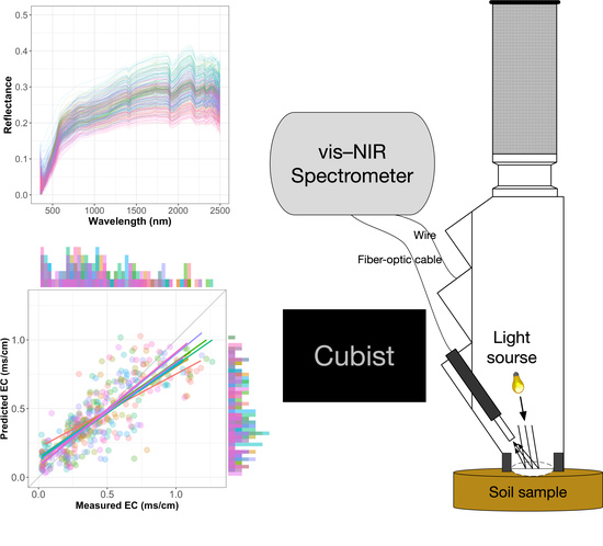
2.2. Spectroscopic Measurements

According to the procedure outlined by Viscarra Rossel et al. [14], the soil vis–NIR spectra were manually measured using a portable Labspec® spectrometer (PaNalytic, Boulder, CO, USA), which has a high-intensity contact probe connected to an external fiber-optic cable. The contact probe measures a spot with a diameter of 10 nm and is designed to reduce errors brought on by stray light. The spectra extending from 350 to 2500 nm were recorded at a 1 nm sampling interval. Each sample, with particle size ≤2 mm was placed in a petri dish (5 cm in diameter and 1 cm in-depth), and then its surface was gently flattened without smearing. Every ten measurements, the spectrometer was re-calibrated using a Spectralon® white reference with a 99% reflectance. Thirty spectra were averaged into one spectrum as the final spectra data for each soil sample.

2.3. Pre-Processing of Spectra

Only the spectra between the wavelength ranges of 400–2450 nm were chosen in order to remove the noise at the borders of each spectrum. The spectra were downscaled to intervals of 10 nm due to their high collinearity. The reflectance of the first wavelength for each spectrum was then subtracted, setting the spectra to a baseline. Savitzky–Golay [20] combined with first derivative smoothing (SG+1D), which are widely used to further minimise the noise and improve the signals. A second order polynomial and a 11 size window, was employed by SG+1D [21]. The resultant spectra were scaled and centred before modelling. Although other pre-processing methods were tested, none were taken into account for this research, as they marginally improved model performance. The R package “prospectr” [22] was used to pre-process all of the soil spectra.

2.4. Modelling Soil’s Electrical Conductivity

Estimating the soil salinity from the spectra requires calibration using accurately measured salinity. A number of multivariate techniques were implemented, and their performances were compared. The partial least-squares regression (PLSR), a linear modeling technique that has grown to be a standard against those new modelling approaches, was one of the three methods employed. The random forest (RF) and the Cubist were the other two “machine learning” techniques. Chen et al. [23] has suggested that utilizing k-fold cross-validation might result in a more reliable evaluation of spectral prediction models when working with small data sets of dozens to hundreds of observations. Therefore, for all models, a 10-fold cross-validation was performed using the same dataset divided by sample ID. To specify the 10 folds in models of RF and Cubist, information of splits was extracted from the PLSR model using “index” and “indexOut” in caret’s “trainControl” function.

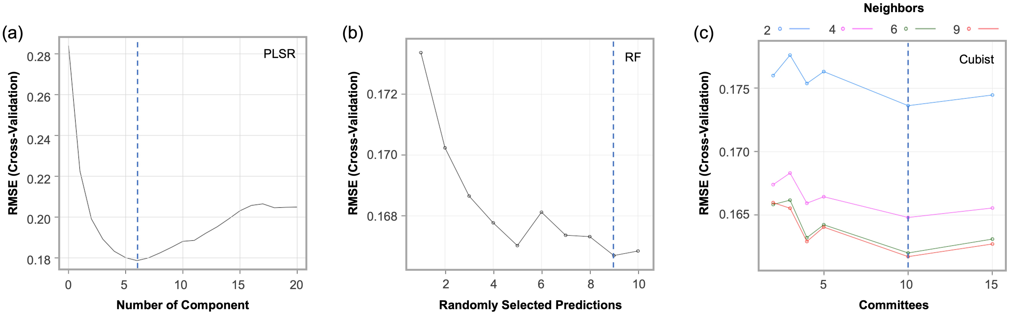
2.4.1. Partial Least-Squares Regression (PLSR)

The PLSR, created by Wold et al. [24], is currently regarded as one of the most well-known multivariate methods for spectral calibration and validation. By choosing successive orthogonal components from the variance–covariance matrix to maximise the covariance between the predictors, it reduces the number of variables to a smaller set of predictors. The optimal number of calibration variables to reduce the prediction error variance was carried out using the 10-fold cross-validation by randomly split [25]. The PLSR model was developed using the R package “pls” and the number of components used for regression was set at maximum value of 20. The featured variables were subjected to the Variable importance in the projection (VIP), with a threshold of 1, which was commonly used [26]. Bands with larger values of VIP than 1 were considered to have a significant role in the model development [27,28].

2.4.2. Random Forest (RF)

The RF is an ensemble learning method that handles classification and regression issues by using top-down and binary splits in a large number of uncorrelated trees (models). It builds each tree randomly and uses bagging (bootstrapping aggregation) to produce an uncorrelated forest of trees, whose prediction is more accurate than that of any single tree [29]. The RF analysis was performed using the “randomForest” of the R package [30]. Two key parameters for RF were optimised as follows: mtry (the number of variables tested at each split) and the ntree (the numerous trees in the forest). According to our previous investigations [23,31,32], they were set to 10 and 500, respectively. The “varImp” function of the “caret” package was used to determine the variable importance by ranking the the node’s purity (IncNodePurity) and the importance of the mean squared error (% IncMSE) in R [33,34].

2.4.3. Cubist

The Cubist is a model tree algorithm based on the M5 methodology [35]. This algorithm splits the variable space into smaller regions and creates multivariate linear least-squares model for each partition by subdividing the variable space into smaller sections. It separates the data into subsets with properties similar to their characteristics (spectra in this case) when the conditions in each rule are met [36]. The analysis for this study uses the R package “Cubist”. To tune the models, different combinations of 2, 3, 4, 5, 10, 15 committees and 2, 4, 6, 9 neighbors were examined. The frequency of each variable used in developing the linear models of the Cubist was calculated in order to quantify the relative importance of the variables and identify the controls. This was accomplished using the “varImp” function of the “caret” package of the R software [30].

2.5. Accuracy Assessment

The approach described by Li et al. [13] was used to evaluate and compare the performances of the studied models. This approach included the use of coefficient of determination ( R 2 ) to evaluate the Pearson correlation between the measurements and the predictions, the root mean square error (RMSE) to assess the goodness of the estimations, and the ratio of performance to inter-quartile distance (RPIQ) to evaluate the efficacy of the developed model for non-normal data distribution [37]. In this study, chemometric analysis and mathematical preprocessing of the data were conducted with R software [38].

3. Results

3.1. Soil Samples Characterization

Table 1 displays the fundamental statistics of the soil samples’ EC and pH for the research area. The EC spanned a wide range from 0.02 to 1.26 with a relatively low average of 0.43. On the other hand, the pH encompassed a range from 6.96 to 8.74, with an average of 8.03. The statistics of the soil EC for ten folds are given in Section 3.2.

3.2. Characterization of Soil Spectra

Figure 1a shows the vis–NIR spectra of each sample. The bright colour over the black background illustrates the greater density between reflectance and wavelength. All of the shapes of the spectra are quite similar, with few differences in the visible range (400–780 nm) and two different patterns in the short-wave NIR range (780–1100 nm), known to the absorptions features of Fe-oxides in soils. With the wavelength continually increasing, the light colour span into a broader range and varied over the near-infrared regions. While clay minerals such as kaolinite are dominant at 2200 nm in the NIR range (1100–2450 nm), the well-defined absorption bands near 1400 and 1900 nm are associated with the overtones of O–H and H–O–H stretch vibration of free water [39,40]. Evidence can be observed in the upper portion of Figure 1a, which represents the spectra pre-processed by SG+1D.
Figure 1b shows the correlation coefficient map between EC and reflectance throughout the wavelength used in this study; lighter colours denote postive correlations, and darker colours negative ones. In general, the spectral wavelengths from the soil samples are often significantly correlated with each other in the 400–2450 nm range. The first line of the map was extracted and shown on the upper figure. Both positive and negative linear correlations are presented with EC throughout the entire spectral regions, which ranged from 0.5 (e.g., peaks at 450 nm and 1350 nm) to −0.5 (e.g., valleys at 900 nm and 2100 nm).
Figure 2a shows the descriptive statistics of the soil EC from 10-folds. There were 40 samples for the lead seven folds and 39 samples for each other fold. All folds span in a similar distribution with a mean EC of around 0.44 mS/cm, except for folds 3, 5, and 7, which have a relatively narrower range compared to the others. The reflectance spectra were decomposed by a principal component analysis (PCA) in order to summarise and examine their structure. For the spectra from 10 folds, Figure 2b displays the scatter of the first two principal component scores shown against one another. About 34% of the overall variation of the spectra was made up of these two prominent components. The three soil types stated previously (see Section 2.1) were somewhat clustered into three with some overlap.

3.3. Spectroscopic Model Evaluation and Estimation

Figure 3 clearly demonstrated that which and how many variables to use in this study. The results demonstrate that considering the PLSR calibration model, six factors had the lowest RMSE (0.18 mS/cm, Figure 3a). On the other hand, the nine variables were used for the RF calibration model, as they gave the lowest RMSE (Figure 3b). The best model for Cubist was obtained when neighbors was 9 and committees was 10 (Figure 3c).
As shown in Figure 4, all the three models successfully estimated the soil EC value. Nevertheless, the Cubist produced the best estimation of EC ( R 2 = 0.67, RMSE = 0.16 mS/cm, RPIQ = 2.28). Furthermore, for samples with an EC value greater than 0.8 mS/cm, the projected EC values were more centred at the 1:1 line than that of both PLSR and RF. Estimates of soil salinity from PLSR were the least accurate ( R 2 = 0.60, RMSE = 0.18 mS/cm, RPIQ = 2.06). The histograms revealed that, in comparison to PLSR and RF, the projected EC values in the Cubist showed better agreement with the measured EC. Additionally, the EC value greater than 0.8 mS/cm was frequently underestimated using PLSR. Given that PLSR is a linear model, the observed significant improvement in RF and Cubist predictions suggests that these models can handle complex nonlinear relationships, such as the one between soil salinity and its reflectance.

3.4. Relative Importance of Variants

The VIP scores of the PLSR model are shown in Figure 5a. Both vis and NIR range contributed to the relevant variables for the estimation of EC by the PLSR model. According to the VIP scores, the most important wavelengths for the soil salinity prediction model were the wavelengths around 1380 nm. The peaks of VIPs (greater than 1) near 470 nm, 700 nm, 900 nm, 1680 nm, 1950 nm, and 2200 nm were also important for modelling. Some of these wavelengths may be connected to the metal–OH bonds, the OH stretch, electronic absorptions, etc.
The variable importance of each variants is shown in Figure 5b,c for the predictions of soil salinity made by IncNodePurity for RF and Conditions for Cubist. The bigger the increase in node purity, the more important the feature (variable). Moreover, the more attribute usage for rule conditions, the more important the variable. To allow a fair comparison between the models, top eight most important variables were chosen for evaluation. The 420 nm, 460–480 nm, and 1360–1390 nm were important when estimating soil EC for the RF model. This contributed to the positive correlations between EC and the above-mentioned wavelengths (Figure 1b). These ranges were also used in the PLSR model, which might be the reason why similar prediction accuracies were obtained by both PLSR and RF models for the estimation of EC.

4. Discussion

Soil salinity, as one of the important properties of soil, does not have an associated unique spectral waveband. The strong correlations, shown in upper Figure 1b, around the 450 nm are associated with color, whereas around the 900 nm, 1350 nm and 2100 nm are located in the three primary water absorption zones in the NIR regions of the spectrum [41]. Strong correlations between spectral variables are known as multicollinearity, which is a typical issue in the estimate of soil parameters using the vis–NIR spectrum.
The most important wavelengths around 1380 nm for PLSR model (Figure 5a), supports the evidence given by Zovoko et al. [42]. It can be partially attributed to the structural O–H stretching mode’s first overtone and H–O–H vibration of water adsorbing on mineral surfaces [43,44]. Some wavelengths in the vis range were also found to be important in this study. In contrast, Zovoko et al. [42] found that this contribution was only in the NIR range. This might be because the various settings and soil types, which affect the ability of spectroscopy and chemometrics to predict EC values [45,46].
Surprisingly, the Cubist model did not use spectra in the 420–480 nm range, as its top eight most important variables ( Figure 5c), although these regions were significantly correlated to the soil EC. For Cubist, the 1370 nm and 1380 nm were used as a comparison with PLSR and RF models. The 1430 nm was used mainly because it is also located around 1400 nm region that corresponds to EC (Figure 1b). On the other hand, the 1680 nm and 1950 nm were also used for Cubist, due to overtones of C–H and C–OH and O–H vibrations, as demonstrated by Viscarra Rossel et al. [14]. Likewise, the 1950 nm wavelength considered as one of the important variables for EC estimation has similar findings to Mousavi et al. [47]. The regions around 1400 nm and 1900 nm, caused by the confluence of molecular free water and overtones, were considered as the association of soil salt content due to their role in the overall contribution from the absorptions [48].
However, when compared to PLSR and RF models, differences are particularly evident at 610 nm and 790 nm, which Cubist used for modelling. A high negative correlation was observed between EC and the spectral reflectance in the 600–800 nm region (Figure 1b). The results indicated that the measured spectral reflectance near 610 nm and 790 nm, which are related to iron oxides, are important bands to predict soil EC by the Cubist model, even if the EC had a lower value range.
It should be noted that the modelling method and parameters’ optimisation proposed in this study are only applicable to vis–NIR reflectance spectral data and low soil EC values. Despite the encouraging results, it is acknowledged that the relative importance of variance would change with the parameters, a possible factor that affects the interpretation of the machine learning model.

5. Conclusions

The present study evaluated the performance of low soil EC prediction using vis–NIR spectra in southern Xinjiang, China. The prediction accuracy among PLSR, RF and Cubist methods were compared and evaluated. The 10-fold cross-validation demonstrated that:
  • Both linear algorithm (PLSR) and nonlinear algorithms (RF, and Cubist) could generate effective chemometrics models;
  • The Cubist gave a much better model performance for soil EC prediction compared to the PLSR and RF model;
  • The water adsorption regions of reflectance spectra (near 1400 and 1900 nm) are highly relevant to soil EC estimation;
  • The 610 nm and 790 nm have great potential for predicting low soil EC values when employing the Cubist model.
It is advised to use the Cubist as the optimum modelling tool to estimate low soil salinity based on the findings of this study. To fully identify the successful in situ measurement of soil salinity or EC, however, more research is required.

Author Contributions

Writing—original draft preparation, J.P.; writing—review and editing, S.L., R.S.M., H.L. and L.F.; methodology, J.P. and S.L.; data collection, C.F. and D.L.; data analysis, J.S. and Y.W.; study site expert, Q.J. and H.L.; supervision, S.L. All authors have read and agreed to the published version of the manuscript.

Funding

This research was funded by the Tarim University President’s Fund, grant number “TDZKCX202205, and TDZKSS202227”; the National Key Research and Development Program of China, grant number “2018YFE0107000”; the National Science Foundation of China, grant number “42071068 and 41061031”; and the Chinese Universities Scientific Fund, grant number “ZNLH201904”.

Conflicts of Interest

The authors declare no conflict of interest.

References

  1. Farifteh, J.; Van der Meer, F.; Atzberger, C.; Carranza, E.J.M. Quantitative analysis of salt-affected soil reflectance spectra: A comparison of two adaptive methods (PLSR and ANN). Remote Sens. Environ. 2007, 110, 59–78. [Google Scholar] [CrossRef]
  2. Abbas, A.; Khan, S.; Hussain, N.; Hanjra, M.A.; Akbar, S. Characterizing soil salinity in irrigated agriculture using a remote sensing approach. Phys. Chem. Earth 2013, 55, 43–52. [Google Scholar] [CrossRef]
  3. Peng, J.; Biswas, A.; Jiang, Q.; Zhao, R.; Hu, J.; Hu, B.; Shi, Z. Estimating soil salinity from remote sensing and terrain data in southern Xinjiang Province, China. Geoderma 2019, 337, 1309–1319. [Google Scholar] [CrossRef]
  4. Liu, Y.; Zhang, F.; Wang, C.; Wu, S.; Liu, J.; Xu, A.; Pan, K.; Pan, X. Estimating the soil salinity over partially vegetated surfaces from multispectral remote sensing image using non-negative matrix factorization. Geoderma 2019, 354, 113887. [Google Scholar] [CrossRef]
  5. Li, H.Y.; Shi, Z.; Webster, R.; Triantafilis, J. Mapping the three-dimensional variation of soil salinity in a rice-paddy soil. Geoderma 2013, 195, 31–41. [Google Scholar] [CrossRef]
  6. Huang, J.; Taghizadeh-Mehrjardi, R.; Minasny, B.; Triantafilis, J. Modeling soil salinity along a hillslope in Iran by inversion of EM38 data. Soil Sci. Soc. Am. J. 2015, 79, 1142–1153. [Google Scholar] [CrossRef]
  7. Jiang, Q.; Peng, J.; Biswas, A.; Hu, J.; Zhao, R.; He, K.; Shi, Z. Characterising dryland salinity in three dimensions. Sci. Total Environ. 2019, 682, 190–199. [Google Scholar] [CrossRef] [PubMed]
  8. Heil, K.; Schmidhalter, U. Theory and Guidelines for the Application of the Geophysical Sensor EM38. Sensors 2019, 19, 4293. [Google Scholar] [CrossRef] [PubMed]
  9. Khongnawang, T.; Zare, E.; Zhao, D.; Srihabun, P.; Triantafilis, J. Three-dimensional mapping of clay and cation exchange capacity of sandy and infertile soil using EM38 and inversion software. Sensors 2019, 19, 3936. [Google Scholar] [CrossRef] [PubMed]
  10. Tziolas, N.; Tsakiridis, N.; Ben-Dor, E.; Theocharis, J.; Zalidis, G. A memory-based learning approach utilizing combined spectral sources and geographical proximity for improved VIS-NIR-SWIR soil properties estimation. Geoderma 2019, 340, 11–24. [Google Scholar] [CrossRef]
  11. Minasny, B.; McBratney, A.B.; Bellon-Maurel, V.; Roger, J.M.; Gobrecht, A.; Ferrand, L.; Joalland, S. Removing the effect of soil moisture from NIR diffuse reflectance spectra for the prediction of soil organic carbon. Geoderma 2011, 167–168, 118–124. [Google Scholar] [CrossRef]
  12. Ji, W.; Viscarra Rossel, R.A.; Shi, Z. Accounting for the effects of water and the environment on proximally sensed vis-NIR soil spectra and their calibrations. Eur. J. Soil Sci. 2015, 66, 555–565. [Google Scholar] [CrossRef]
  13. Li, S.; Viscarra Rossel, R.A.; Webster, R. The cost-effectiveness of reflectance spectroscopy for estimating soil organic carbon. Eur. J. Soil Sci. 2022, 73, e13202. [Google Scholar] [CrossRef]
  14. Viscarra Rossel, R.A.; Behrens, T.; Ben-Dor, E.; Brown, D.J.; Demattê, J.A.M.; Shepherd, K.D.; Shig, Z.; Stenbergh, B.; Stevens, A.; Ji, W.; et al. A global spectral library to characterize the world’s soil. Earth-Sci. Rev. 2016, 155, 198–230. [Google Scholar] [CrossRef]
  15. Soriano-Disla, J.M.; Janik, L.J.; Viscarra Rossel, R.A.; Macdonald, L.M.; McLaughlin, M.J. The performance of visible, near-, and mid-infrared reflectance spectroscopy for prediction of soil physical, chemical, and biological properties. Appl. Spectrosc. Rev. 2014, 49, 139–186. [Google Scholar] [CrossRef]
  16. Singh, K.; Majeed, I.; Panigrahi, N.; Vasava, H.B.; Fidelis, C.; Karunaratne, S.; Field, D.J. Near infrared diffuse reflectance spectroscopy for rapid and comprehensive soil condition assessment in smallholder cacao farming systems of Papua New Guinea. Catena 2019, 183, 104185. [Google Scholar] [CrossRef]
  17. Shahrayini, E.; Noroozi, A.A.; Eghbal, M.K. Prediction of Soil Properties by Visible and Near-Infrared Reflectance Spectroscopy. Eur. J. Soil Sci. 2020, 53, 1760–1772. [Google Scholar] [CrossRef]
  18. Shen, Z.; Ramirez-Lopez, L.; Behrens, T.; Cui, L.; Zhang, M.; Walden, L.; Wetterlindf, J.; Shig, Z.; Sudduth, K.A.; Viscarra Rossel, R.A.; et al. Deep transfer learning of global spectra for local soil carbon monitoring. ISPRS J. Photogramm. 2022, 188, 190–200. [Google Scholar] [CrossRef]
  19. Fan, X.; Liu, Y.; Tao, J.; Weng, Y. Soil salinity retrieval from advanced multi-spectral sensor with partial least square regression. Remote Sens. 2015, 7, 488–511. [Google Scholar] [CrossRef]
  20. Savitzky, A.; Golay, M.J.E. Smoothing and differentiation of data by simplified least squares procedures. Anal. Chem. 1964, 36, 1627–1639. [Google Scholar] [CrossRef]
  21. Hong, Y.; Munnaf, M.A.; Guerrero, A.; Chen, S.; Liu, Y.; Shi, Z.; Mouazen, A.M. Fusion of visible-to-near-infrared and mid-infrared spectroscopy to estimate soil organic carbon. Soil Tillage Res. 2022, 217, 105284. [Google Scholar] [CrossRef]
  22. Stevens, A.; Ramirez-Lopez, L. An Introduction to the Prospectr Package. R Package Version 0.2.6. Available online: https://cran.r-project.org/web/packages/prospectr/vignettes/prospectr.html (accessed on 1 September 2022).
  23. Chen, S.; Xu, H.; Xu, D.; Ji, W.; Li, S.; Yang, M.; Hu, B.; Zhou, Y.; Wang, N.; Arrouays, D.; et al. Evaluating validation strategies on the performance of soil property prediction from regional to continental spectral data. Geoderma 2021, 400, 115159. [Google Scholar] [CrossRef]
  24. Wold, S.; Martens, H.; Wold, H. The Multivariate Calibration Problem in Chemistry Solved by the Pls Method by the PLS Method; Springer: Berlin/Heidelberg, Germany, 1983; pp. 286–293. [Google Scholar]
  25. Martens, H.; Næs, T. Multivariate Calibration; John Wiley & Sons: New York, NY, USA, 1989. [Google Scholar]
  26. Chong, I.G.; Jun, C.H. Performance of some variable selection methods when multicollinearity is present. Chemom. Intell. Lab. Syst. 2005, 78, 103–112. [Google Scholar] [CrossRef]
  27. Hu, B.; Chen, S.; Hu, J.; Xia, F.; Xu, J.; Li, Y.; Shi, Z. Application of portable XRF and VNIR sensors for rapid assessment of soil heavy metal pollution. PLoS ONE 2017, 12, e0172438. [Google Scholar] [CrossRef] [PubMed]
  28. Hu, B.; Bourennane, H.; Arrouays, D.; Denoroy, P.; Lemercier, B.; Saby, N.P. Developing pedotransfer functions to harmonize extractable soil phosphorus content measured with different methods: A case study across the mainland of France. Geoderma 2021, 381, 114645. [Google Scholar] [CrossRef]
  29. Breiman, L. Random forests. Mach. Learn. 2001, 45, 5–32. [Google Scholar] [CrossRef]
  30. Kuhn, M. Building predictive models in R using the caret package. J. Stat. Softw. 2008, 28, 1–26. [Google Scholar] [CrossRef]
  31. Hu, B.; Xue, J.; Zhou, Y.; Shao, S.; Fu, Z.; Li, Y.; Chen, S.; Qi, L.; Shi, Z. Modelling bioaccumulation of heavy metals in soil-crop ecosystems and identifying its controlling factors using machine learning. Environ. Pollut. 2020, 262, 114308. [Google Scholar] [CrossRef] [PubMed]
  32. Wang, N.; Peng, J.; Xue, J.; Zhang, X.; Huang, J.; Biswas, A.; He, Y.; Shi, Z. A framework for determining the total salt content of soil profiles using time-series Sentinel-2 images and a random forest-temporal convolution network. Geoderma 2022, 409, 115656. [Google Scholar] [CrossRef]
  33. Wang, J.; Ding, J.; Yu, D.; Ma, X.; Zhang, Z.; Ge, X.; Teng, D.; Li, X.; Liang, J.; Lizaga, I.; et al. Capability of Sentinel-2 MSI data for monitoring and mapping of soil salinity in dry and wet seasons in the Ebinur Lake region, Xinjiang, China. Geoderma 2019, 353, 172–187. [Google Scholar] [CrossRef]
  34. Yan, F.; Shangguan, W.; Zhang, J.; Hu, B. Depth-to-bedrock map of China at a spatial resolution of 100 meters. Sci. Data 2020, 7, 2. [Google Scholar] [CrossRef] [PubMed]
  35. Quinlan, J.R. Learning with continuous classes. In Proceedings of the Proceedings AI’92, 5th Australian Conference on Artificial Intelligence, Hobart, Tasmania, 16–18 November 1992; Adams, A., Sterling, L., Eds.; World Scientific: Singapore, 1992; pp. 343–348. [Google Scholar]
  36. Viscarra Rossel, R.A.; Webster, R. Predicting soil properties from the Australian soil visible-near infrared spectroscopic database. Eur. J. Soil Sci. 2012, 63, 848–860. [Google Scholar] [CrossRef]
  37. Bellon-Maurel, V.; Fernandez-Ahumada, E.; Palagos, B.; Roger, J.M.; McBratney, A. Critical review of chemometric indicators commonly used for assessing the quality of the prediction of soil attributes by NIR spectroscopy. Trends Anal. Chem. 2010, 29, 1073–1081. [Google Scholar] [CrossRef]
  38. R Core Team. R: A Language and Environment for Statistical Computing; R Foundation for Statistical Computing: Vienna, Austria, 2020. [Google Scholar]
  39. Clark, R.N.; King, T.V.; Klejwa, M.; Swayze, G.A.; Vergo, N. High spectral resolution reflectance spectroscopy of minerals. J. Geophys. Res. Solid Earth 1990, 95, 12653–12680. [Google Scholar] [CrossRef]
  40. Ben-Dor, E.; Chabrillat, S.; Demattê, J.A.M.; Taylor, G.R.; Hill, J.; Whiting, M.L.; Sommer, S. Using imaging spectroscopy to study soil properties. Remote Sens. Environ. 2009, 113, S38–S55. [Google Scholar] [CrossRef]
  41. Li, S.; Shi, Z.; Chen, S.; Ji, W.; Zhou, L.; Yu, W.; Webster, R. In situ measurements of organic carbon in soil profiles using vis-NIR spectroscopy on the Qinghai–Tibet plateau. Environ. Sci. Technol. 2015, 49, 4980–4987. [Google Scholar] [CrossRef] [PubMed]
  42. Zovko, M.; Romić, D.; Colombo, C.; Di Iorio, E.; Romić, M.; Buttafuoco, G.; Castrignanò, A. A geostatistical Vis-NIR spectroscopy index to assess the incipient soil salinization in the Neretva River valley, Croatia. Geoderma 2018, 332, 60–72. [Google Scholar] [CrossRef]
  43. Bishop, J.L.; Pieters, C.M.; Edwards, J.O. Infrared spectroscopic analyses on the nature of water in montmorillonite. Clays Clay Miner. 1994, 42, 702–716. [Google Scholar] [CrossRef]
  44. Stenberg, B.; Viscarra Rossel, R.A.; Mouazen, A.M.; Wetterlind, J. Visible and near infrared spectroscopy in soil science. Adv. Agron. 2010, 107, 163–215. [Google Scholar] [CrossRef]
  45. Zornoza, R.; Guerrero, C.; Mataix-Solera, J.; Scow, K.M.; Arcenegui, V.; Mataix-Beneyto, J. Near infrared spectroscopy for determination of various physical, chemical and biochemical properties in Mediterranean soils. Soil Biol. Biochem. 2008, 40, 1923–1930. [Google Scholar] [CrossRef] [PubMed] [Green Version]
  46. Minasny, B.; Tranter, G.; McBratney, A.B.; Brough, D.M.; Murphy, B.W. Regional transferability of mid-infrared diffuse reflectance spectroscopic prediction for soil chemical properties. Geoderma 2009, 153, 155–162. [Google Scholar] [CrossRef]
  47. Mousavi, F.; Abdi, E.; Knadel, M.; Tuller, M.; Ghalandarzadeh, A.; Bahrami, H.A.; Majnounian, B. Combining Vis–NIR spectroscopy and advanced statistical analysis for estimation of soil chemical properties relevant for forest road construction. Soil Sci. Soc. Am. J. 2021, 85, 1073–1090. [Google Scholar] [CrossRef]
  48. Nawar, S.; Buddenbaum, H.; Hill, J.; Kozak, J. Modeling and mapping of soil salinity with reflectance spectroscopy and landsat data using two quantitative methods (PLSR and MARS). Remote Sens. 2014, 6, 10813–10834. [Google Scholar] [CrossRef] [Green Version]
Figure 1. The reflectance spectra (by density) with preprocessed spectra (a), and correlation coefficient maps between measured EC and reflectance of wavelengths pairs (b).
Remotesensing 14 04448 g001
Figure 2. Boxplots of EC (a) and scatter plots of the scores of second principal component (PC2) against those of the first principal component (PC1) for soil reflectance spectra (b) from 10 folds. The ellipse is shown in 95% level.
Remotesensing 14 04448 g002
Figure 3. Root mean-square errors (RMSE) of cross-validation for soil EC, showing the best number of component, predictors and committees to use in each of the PLSR (a), RF (b), and Cubist (c) models.
Remotesensing 14 04448 g003
Figure 4. Observed vs. predicted soil EC with the assessment of statistics from a 10-fold cross-validation of PLSR (a), RF (b), and Cubist (c) models. Values out and in brackets are mean, minimum and maximum values, respectively. The solid 1:1 line in grey is drawn for reference. Top and right histograms show the distributions of measured and predicted EC values.
Remotesensing 14 04448 g004
Figure 5. The variables’ importance of models for EC from PLSR (a), RF (b), and Cubist (c).
Remotesensing 14 04448 g005
Table 1. Statistics of EC (in mS/cm) and pH.
PropertyMin.1st Q.MedianMean3rd Q.Max.Skew
EC0.020.240.370.430.611.260.74
pH6.967.888.068.038.228.74−0.71
Note: Min, minimum; Max, maximum; Q, Quartile; Skew, skewness coefficient.
Publisher’s Note: MDPI stays neutral with regard to jurisdictional claims in published maps and institutional affiliations.

