
The Spatio-Temporal Variability in the Radiative Forcing of Light-Absorbing Particles in Snow of 2003–2018 over the Northern Hemisphere from MODIS

 , , , , and
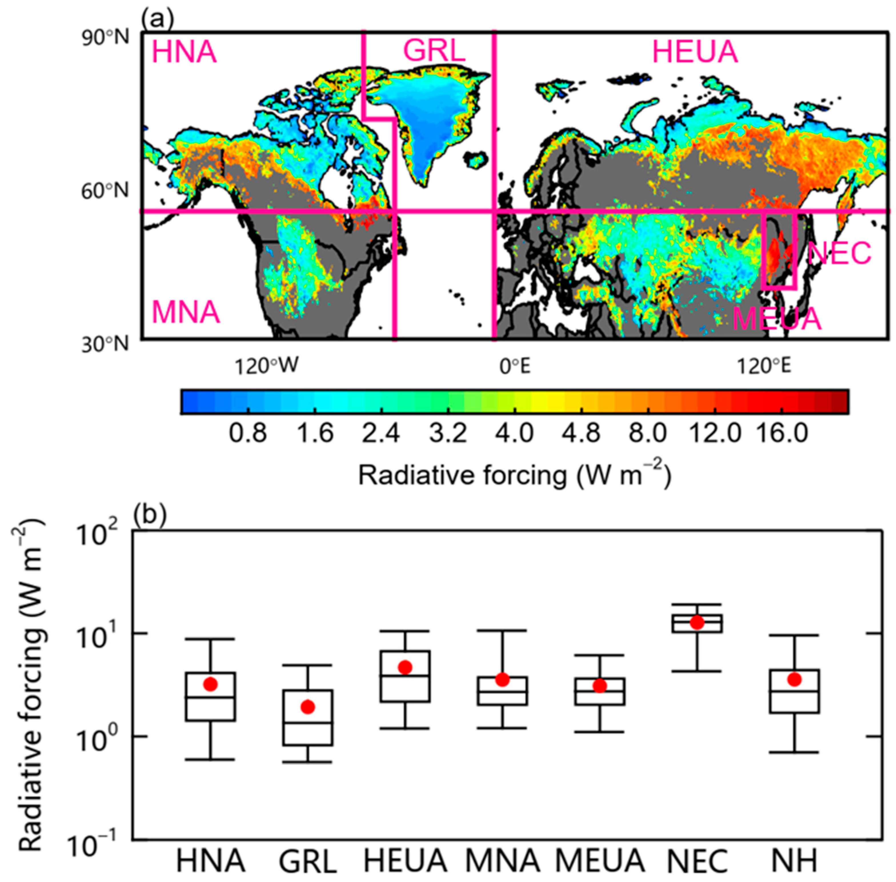
Abstract
:1. Introduction
2. Materials and Methods
2.1. MODIS Datasets
2.2. CERES Datasets
2.3. ERA5 Snow Water Equivalent Data
2.4. Radiation Transfer Models
2.5. Radiative Forcing Retrievals
2.5.1. Retrievals of Blue-Sky Albedo from MODIS
2.5.2. Identification of Snow-Covered Area and Retrievals of Snow Albedo
2.5.3. Retrievals of Snow Grain Sizes
2.5.4. Retrieval of RF
2.6. Attribution of Spatio-Temporal Variability in Radiative Forcing
2.7. Sensitivity of Interannual Variation of RF
3. Results
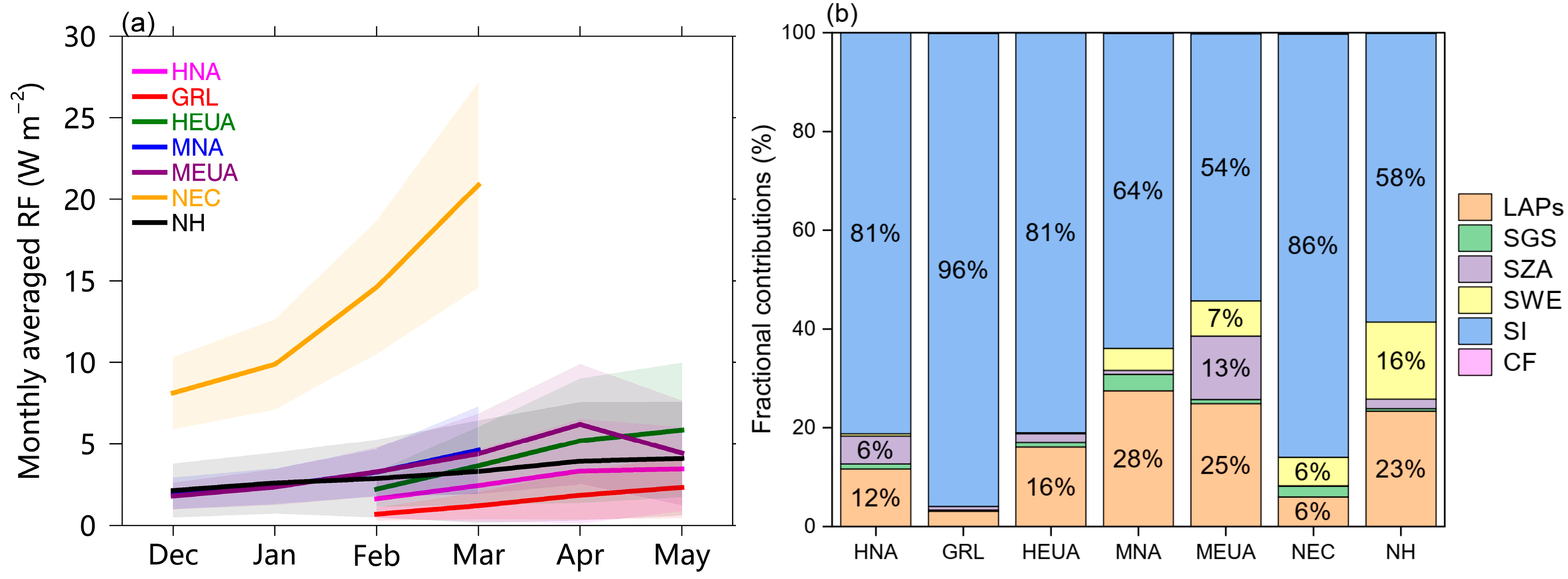
3.1. Spatial Distributions of RF in the Northern Hemisphere
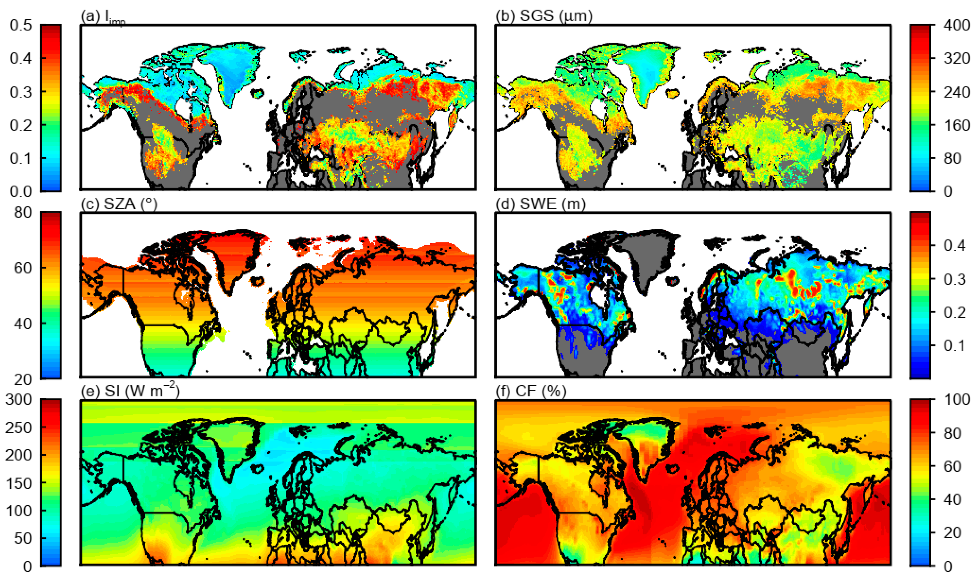
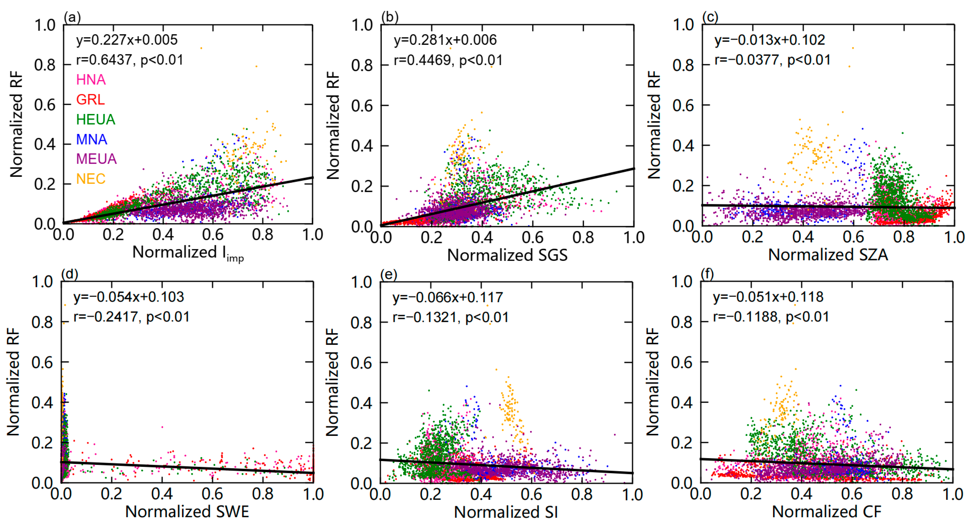
3.2. Attribution of Spatial Variability in RF
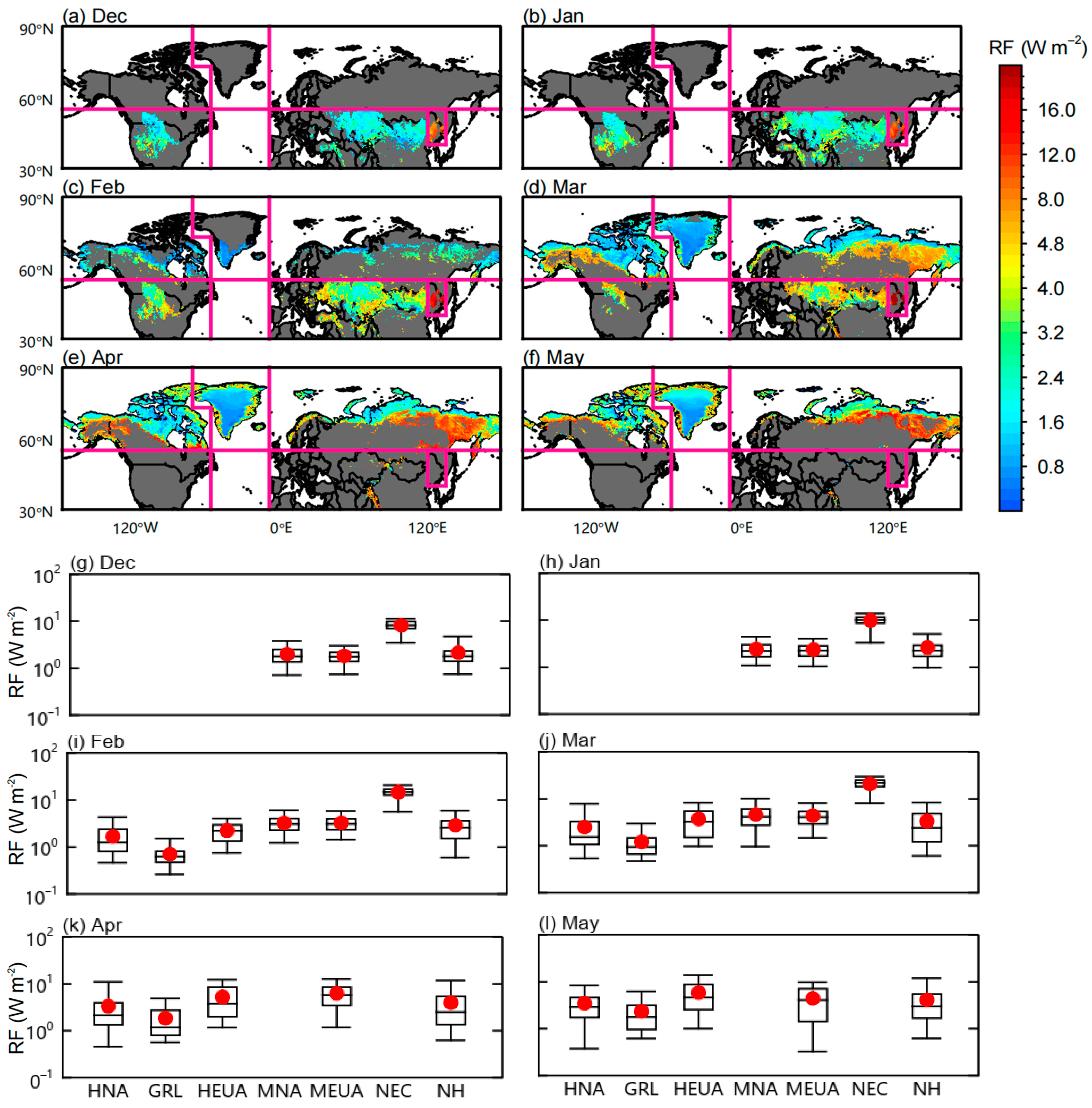
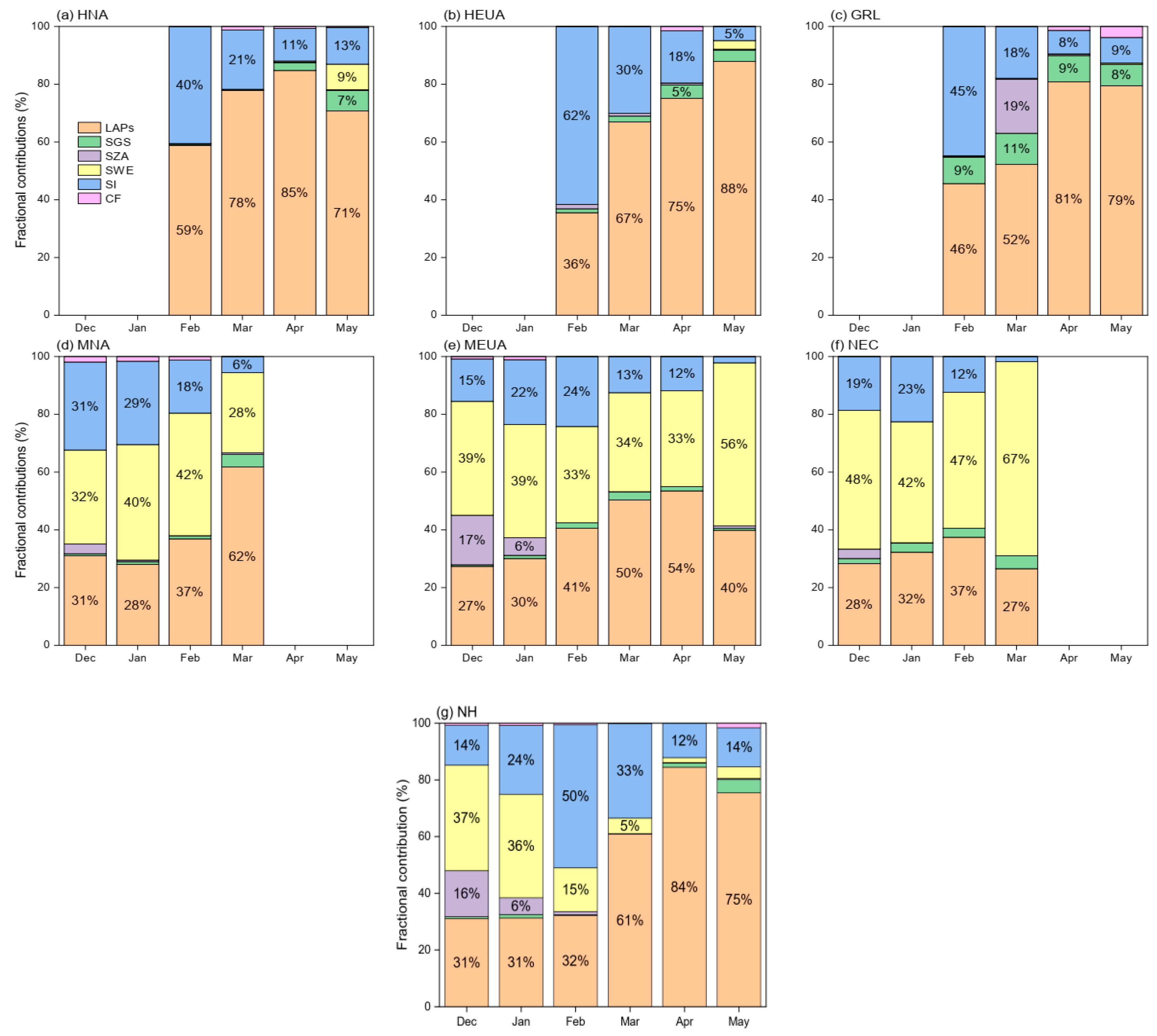
3.3. Seasonal Variability and Attribution in RF
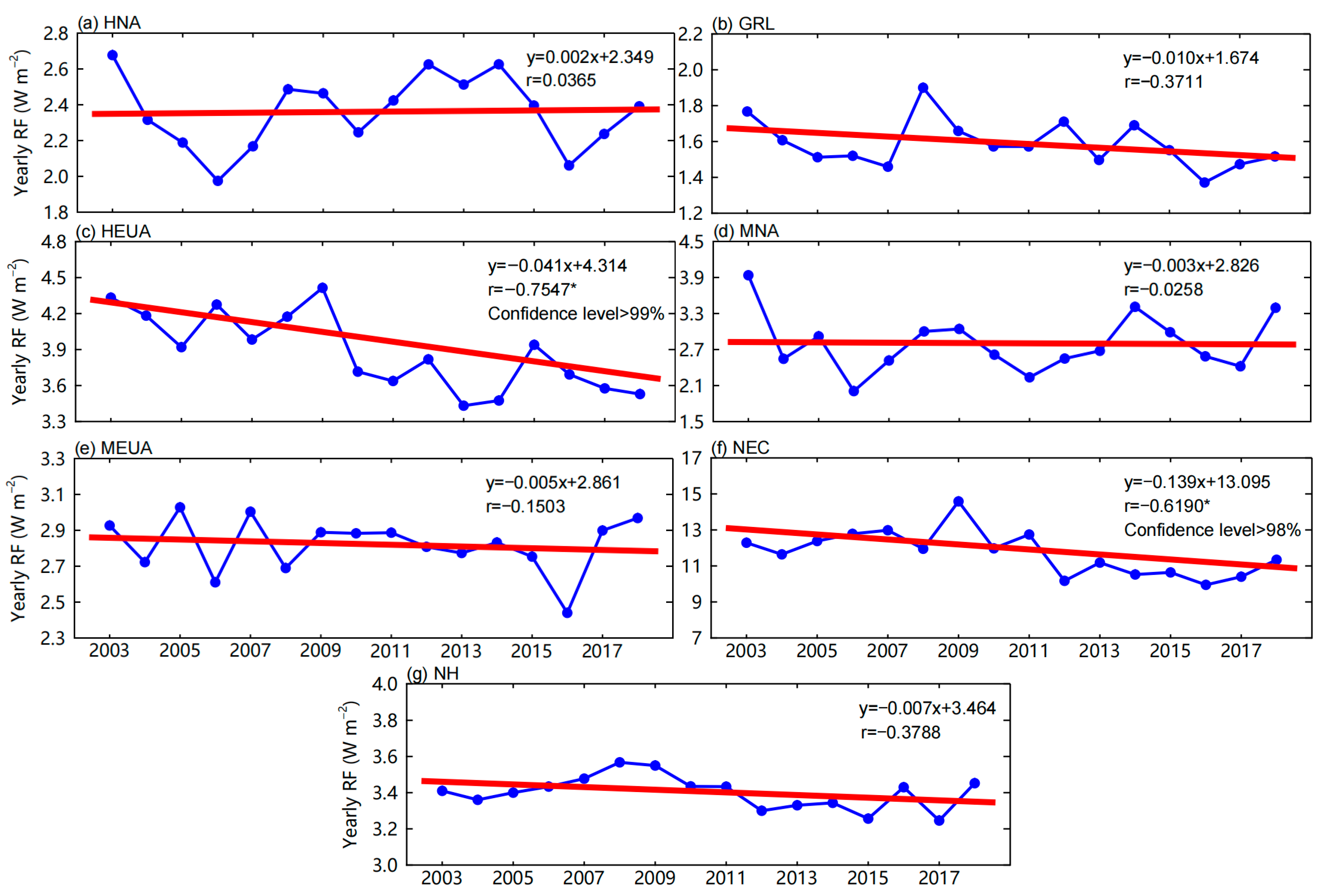
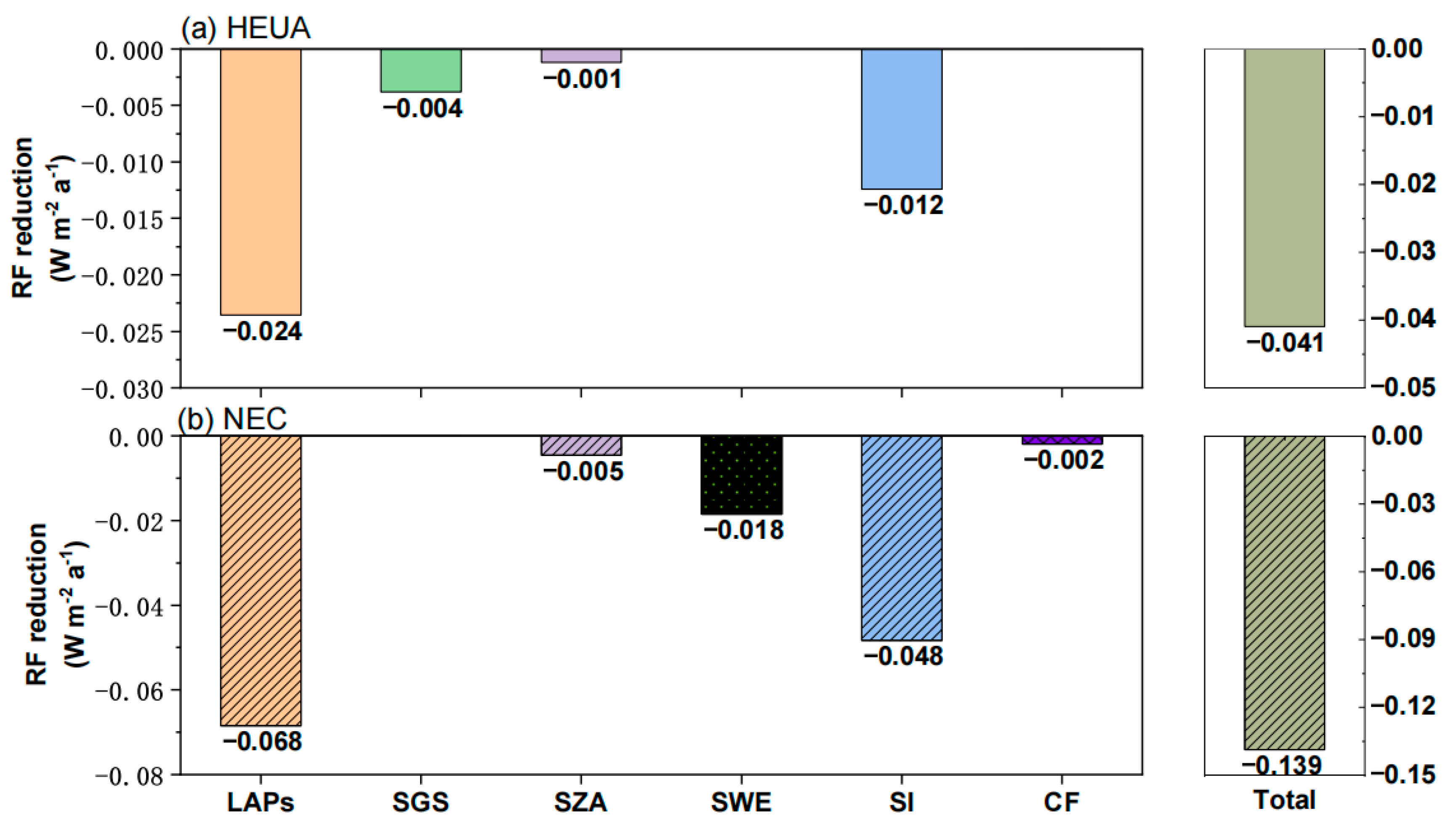
3.4. Interannual RF Variance and Attribution
4. Discussion
5. Conclusions
Supplementary Materials
Author Contributions
Funding
Data Availability Statement
Acknowledgments
Conflicts of Interest
Abbreviations
| ACRONYM | Definition |
| BC | Black carbon |
| BHR | Bi-hemispherical reflectance |
| BRDF | Bidirectional Reflectance Distribution Function |
| CAM5 | Community Atmosphere Model version 5 |
| CERES | Clouds and the Earth’s Radiant Energy System |
| CF | Cloud fraction |
| DHR | Directional hemispherical reflectance |
| ECMWF | European Centre for Medium-Range Weather Forecasts |
| FSC | Fractional Snow Cover |
| GRL | Greenland |
| HEUA | High-latitude Eurasia |
| HNA | High-latitude North America |
| IMS | Interactive Multisensor Snow and Ice Mapping System |
| ISCA | Identified snow-covered area |
| LAPS | Light-absorbing particles |
| MEUA | Mid-latitude Eurasia |
| MNA | Mid-latitude North America |
| MODIS | Moderate Resolution Imaging Spectroradiometer |
| NDSI | Normalized Difference Snow Index |
| NEC | Northeastern China |
| NIR | Near-infrared |
| OC | Organic carbon |
| OLI | Operational Land Imager |
| RF | Radiative forcing |
| SBDART | The Santa Barbara DISORT Atmospheric Radiative Transfer |
| SGS | Snow grain sizes |
| SI | Solar irradiance |
| SNICAR | Snow, Ice, and Aerosol Radiative model |
| SNOWPACK | Multilayer, physically based snow-process model |
| SRTM | Shuttle Radar Topography Mission |
| SWE | Snow water equivalent |
| SZA | Solar zenith angle |
| UAV | Unmanned Aerial Vehicle |
References
- Betts, A.K.; Ball, J.H. Albedo over the boreal forest. J. Geophys. Res. Atmos. 1997, 102, 28901–28909. [Google Scholar] [CrossRef] [Green Version]
- Picard, G.; Dumont, M.; Lamare, M.; Tuzet, F.; Larue, F.; Pirazzini, R.; Arnaud, L. Spectral albedo measurements over snow-covered slopes: Theory and slope effect corrections. Cryosphere 2020, 14, 1497–1517. [Google Scholar] [CrossRef]
- Painter, T.H.; Roberts, D.A.; Green, R.O.; Dozier, J. The Effect of Grain Size on Spectral Mixture Analysis of Snow-Covered Area from AVIRIS Data. Remote Sens. Environ. 1998, 65, 320–332. [Google Scholar] [CrossRef]
- Warren, S.G. Optical properties of snow. Rev. Geophys. 1982, 20, 67. [Google Scholar] [CrossRef]
- Warren, S.G. Impurities in Snow: Effects on Albedo and Snowmelt (Review). Ann. Glaciol. 1984, 5, 177–179. [Google Scholar] [CrossRef] [Green Version]
- Mu, Z.; Niu, X.; George, C.; Wang, X.; Huang, R.; Ma, Y.; Pu, W.; Qi, Y.; Fu, P.; Deng, J.; et al. Accumulation of dissolved organic matter in the transition from fresh to aged seasonal snow in an industrial city in NE China. Sci. Total Environ. 2023, 857, 159337. [Google Scholar] [CrossRef]
- Niu, X.; Pu, W.; Fu, P.; Chen, Y.; Xing, Y.; Wu, D.; Chen, Z.; Shi, T.; Zhou, Y.; Wen, H.; et al. Fluorescence characteristics, absorption properties, and radiative effects of water-soluble organic carbon in seasonal snow across northeastern China. Atmos. Chem. Phys. 2022, 22, 14075–14094. [Google Scholar] [CrossRef]
- Zhou, Y.; Wen, H.; Liu, J.; Pu, W.; Chen, Q.; Wang, X. The optical characteristics and sources of chromophoric dissolved organic matter (CDOM) in seasonal snow of northwestern China. Cryosphere 2019, 13, 157–175. [Google Scholar] [CrossRef] [Green Version]
- Zhou, Y.; West, C.P.; Hettiyadura, A.P.S.; Niu, X.; Wen, H.; Cui, J.; Shi, T.; Pu, W.; Wang, X.; Laskin, A. Measurement report: Molecular composition, optical properties, and radiative effects of water-soluble organic carbon in snowpack samples from northern Xinjiang, China. Atmos. Chem. Phys. 2021, 21, 8531–8555. [Google Scholar] [CrossRef]
- Painter, T.H.; Skiles, S.M.; Deems, J.S.; Bryant, A.C.; Landry, C.C. Dust radiative forcing in snow of the Upper Colorado River Basin: 1. A 6 year record of energy balance, radiation, and dust concentrations. Water Resour. Res. 2012, 48, W07521. [Google Scholar] [CrossRef]
- Warren, S.G.; Brandt, R.E. Optical constants of ice from the ultraviolet to the microwave: A revised compilation. J. Geophys. Res. 2008, 113, D14220. [Google Scholar] [CrossRef]
- Shi, T.; Chen, Y.; Xing, Y.; Niu, X.; Wu, D.; Cui, J.; Zhou, Y.; Pu, W.; Wang, X. Assessment of the combined radiative effects of black carbon in the atmosphere and snowpack in the Northern Hemisphere constrained by surface observations. Environ. Sci. Atmos. 2022, 2, 702–713. [Google Scholar] [CrossRef]
- Wang, X.; Shi, T.; Zhang, X.; Chen, Y. An Overview of Snow Albedo Sensitivity to Black Carbon Contamination and Snow Grain Properties Based on Experimental Datasets Across the Northern Hemisphere. Curr. Pollut. Rep. 2020, 6, 368–379. [Google Scholar] [CrossRef]
- Cui, J.; Shi, T.; Zhou, Y.; Wu, D.; Wang, X.; Pu, W. Satellite-based radiative forcing by light-absorbing particles in snow across the Northern Hemisphere. Atmos. Chem. Phys. 2021, 21, 269–288. [Google Scholar] [CrossRef]
- Wielicki, B.A.; Wong, T.; Loeb, N.; Minnis, P.; Priestley, K.; Kandel, R. Changes in Earth’s albedo measured by satellite. Science 2005, 308, 825. [Google Scholar] [CrossRef]
- Wang, X.; Pu, W.; Zhang, X.; Ren, Y.; Huang, J. Water-soluble ions and trace elements in surface snow and their potential source regions across northeastern China. Atmos. Environ. 2015, 114, 57–65. [Google Scholar] [CrossRef]
- Wang, X.; Xu, B.; Ming, J. An overview of the studies on black carbon and mineral dust deposition in snow and ice cores in East Asia. J. Meteorol. Res. 2014, 28, 354–370. [Google Scholar] [CrossRef]
- Wang, X.; Pu, W.; Shi, J.; Bi, J.; Zhou, T.; Zhang, X.; Ren, Y. A comparison of the physical and optical properties of anthropogenic air pollutants and mineral dust over Northwest China. J. Meteorol. Res. 2015, 29, 180–200. [Google Scholar] [CrossRef]
- Dang, C.; Warren, S.G.; Fu, Q.; Doherty, S.J.; Sturm, M.; Su, J. Measurements of light-absorbing particles in snow across the Arctic, North America, and China: Effects on surface albedo. J. Geophys. Res. 2017, 122, 10149–10168. [Google Scholar] [CrossRef]
- Ganey, G.Q.; Loso, M.G.; Burgess, A.B.; Dial, R.J. The role of microbes in snowmelt and radiative forcing on an Alaskan icefield. Nat. Geosci. 2017, 10, 754–759. [Google Scholar] [CrossRef]
- Skiles, S.M.; Painter, T.H.; Deems, J.S.; Bryant, A.C.; Landry, C.C. Dust radiative forcing in snow of the Upper Colorado River Basin: 2. Interannual variability in radiative forcing and snowmelt rates. Water Resour. Res. 2012, 48, W07522. [Google Scholar] [CrossRef]
- Pu, W.; Wang, X.; Wei, H.; Zhou, Y.; Shi, J.; Hu, Z.; Jin, H.; Chen, Q. Properties of black carbon and other insoluble light-absorbing particles in seasonal snow of northwestern China. Cryosphere 2017, 11, 1213–1233. [Google Scholar] [CrossRef] [Green Version]
- Wang, X.; Wei, H.; Liu, J.; Xu, B.; Wang, M.; Ji, M.; Jin, H. Quantifying the light absorption and source attribution of insoluble light-absorbing particles on Tibetan Plateau glaciers between 2013 and 2015. Cryosphere 2019, 13, 309–324. [Google Scholar] [CrossRef] [Green Version]
- Wang, X.; Zhang, X.; Di, W. Development of an improved two-sphere integration technique for quantifying black carbon concentrations in the atmosphere and seasonal snow. Atmos. Meas. Tech. 2020, 13, 39–52. [Google Scholar] [CrossRef] [Green Version]
- Qian, Y.; Wang, H.; Zhang, R.; Flanner, M.G.; Rasch, P.J. A sensitivity study on modeling black carbon in snow and its radiative forcing over the Arctic and Northern China. Environ. Res. Lett. 2014, 9, 064001. [Google Scholar] [CrossRef] [Green Version]
- Young, C.L.; Sokolik, I.N.; Flanner, M.G.; Dufek, J. Surface radiative impacts of ash deposits from the 2009 eruption of Redoubt volcano. J. Geophys. Res. Atmos. 2014, 119, 11,387–11,397. [Google Scholar] [CrossRef]
- Skiles, S.M.; Painter, T.H. Toward Understanding Direct Absorption and Grain Size Feedbacks by Dust Radiative Forcing in Snow with Coupled Snow Physical and Radiative Transfer Modeling. Water Resour. Res. 2019, 55, 7362–7378. [Google Scholar] [CrossRef]
- Skiles, S.M.; Mallia, D.V.; Hallar, A.G.; Lin, J.C.; Lambert, A.; Petersen, R.; Clark, S. Implications of a shrinking Great Salt Lake for dust on snow deposition in the Wasatch Mountains, UT, as informed by a source to sink case study from the 13–14 April 2017 dust event. Environ. Res. Lett. 2018, 13, 124031. [Google Scholar] [CrossRef]
- Pu, W.; Cui, J.; Wu, D.; Shi, T.; Chen, Y.; Xing, Y.; Zhou, Y.; Wang, X. Unprecedented snow darkening and melting in New Zealand due to 2019–2020 Australian wildfires. Fundam. Res. 2021, 1, 224–231. [Google Scholar] [CrossRef]
- Bryant, A.C.; Painter, T.H.; Deems, J.S.; Bender, S.M. Impact of dust radiative forcing in snow on accuracy of operational runoff prediction in the Upper Colorado River Basin. Geophys. Res. Lett. 2013, 40, 3945–3949. [Google Scholar] [CrossRef]
- Di Mauro, B.; Fava, F.; Ferrero, L.; Garzonio, R.; Baccolo, G.; Delmonte, B.; Colombo, R. Mineral dust impact on snow radiative properties in the European Alps combining ground, UAV, and satellite observations. J. Geophys. Res. Atmos. 2015, 120, 6080–6097. [Google Scholar] [CrossRef]
- Chen, W.; Wang, X.; Cui, J.; Cao, X.; Pu, W.; Zheng, X.; Ran, H.; Ding, J. Radiative forcing of black carbon in seasonal snow of wintertime based on remote sensing over Xinjiang, China. Atmos. Environ. 2021, 247, 118204. [Google Scholar] [CrossRef]
- Skiles, S.M.; Flanner, M.; Cook, J.M.; Dumont, M.; Painter, T.H. Radiative forcing by light-absorbing particles in snow. Nat. Clim. Chang. 2018, 8, 964–971. [Google Scholar] [CrossRef]
- Bond, T.C.; Doherty, S.J.; Fahey, D.W.; Forster, P.M.; Berntsen, T.; DeAngelo, B.J.; Flanner, M.G.; Ghan, S.; Kärcher, B.; Koch, D.; et al. Bounding the role of black carbon in the climate system: A scientific assessment. J. Geophys. Res. Atmos. 2013, 118, 5380–5552. [Google Scholar] [CrossRef]
- Kaspari, S.; Painter, T.H.; Gysel, M.; Skiles, S.M.; Schwikowski, M. Seasonal and elevational variations of black carbon and dust in snow and ice in the Solu-Khumbu, Nepal and estimated radiative forcings. Atmos. Chem. Phys. 2014, 14, 8089–8103. [Google Scholar] [CrossRef]
- Skiles, S.M.; Painter, T. Daily evolution in dust and black carbon content, snow grain size, and snow albedo during snowmelt, Rocky Mountains, Colorado. J. Glaciol. 2016, 63, 118–132. [Google Scholar] [CrossRef] [Green Version]
- Zhou, Y.; West, C.P.; Hettiyadura, A.P.S.; Pu, W.; Shi, T.; Niu, X.; Wen, H.; Cui, J.; Wang, X.; Laskin, A. Molecular Characterization of Water-Soluble Brown Carbon Chromophores in Snowpack from Northern Xinjiang, China. Env. Sci. Technol. 2022, 56, 4173–4186. [Google Scholar] [CrossRef]
- Xu, B.; Cao, J.; Hansen, J.; Yao, T.; Joswia, D.R.; Wang, N.; Wu, G.; Wang, M.; Zhao, H.; Yang, W.; et al. Black soot and the survival of Tibetan glaciers. Proc. Natl. Acad. Sci. USA 2009, 106, 22114–22118. [Google Scholar] [CrossRef] [Green Version]
- Kang, S.; Zhang, Q.; Zhang, Y.; Guo, W.; Ji, Z.; Shen, M.; Wang, S.; Wang, X.; Tripathee, L.; Liu, Y.; et al. Warming and thawing in the Mt. Everest region: A review of climate and environmental changes. Earth-Sci. Rev. 2022, 225, 103911. [Google Scholar] [CrossRef]
- Zhao, C.; Hu, Z.; Qian, Y.; Ruby Leung, L.; Huang, J.; Huang, M.; Jin, J.; Flanner, M.G.; Zhang, R.; Wang, H.; et al. Simulating black carbon and dust and their radiative forcing in seasonal snow: A case study over North China with field campaign measurements. Atmos. Chem. Phys. 2014, 14, 11475–11491. [Google Scholar] [CrossRef]
- Qi, L.; Li, Q.; Li, Y.; He, C. Factors controlling black carbon distribution in the Arctic. Atmos. Chem. Phys. 2017, 17, 1037–1059. [Google Scholar] [CrossRef] [Green Version]
- Schaaf, C.B.; Gao, F.; Strahler, A.H.; Lucht, W.; Li, X.W.; Tsang, T.; Strugnell, N.C.; Zhang, X.Y.; Jin, Y.F.; Muller, J.P.; et al. First operational BRDF, albedo nadir reflectance products from MODIS. Remote Sens. Environ. 2002, 83, 135–148. [Google Scholar] [CrossRef] [Green Version]
- Schaaf, C.B.; Wang, Z.; Strahler, A.H. Commentary on Wang and Zender—MODIS snow albedo bias at high solar zenith angles relative to theory and to in situ observations in Greenland. Remote. Sens. Environ. 2011, 115, 1296–1300. [Google Scholar] [CrossRef]
- Wang, Z.; Schaaf, C.B.; Sun, Q.; Shuai, Y.; Román, M.O. Capturing rapid land surface dynamics with Collection V006 MODIS BRDF/NBAR/Albedo (MCD43) products. Remote. Sens. Environ. 2018, 207, 50–64. [Google Scholar] [CrossRef]
- Jin, Y.; Schaaf, C.B.; Gao, F.; Li, X.; Strahler, A.H.; Lucht, W.; Liang, S. Consistency of MODIS surface bidirectional reflectance distribution function and albedo retrievals: 1. Algorithm performance. J. Geophys. Res. 2003, 108, 4158. [Google Scholar] [CrossRef]
- Jin, Y.; Schaaf, C.B.; Woodcock, C.E.; Gao, F.; Li, X.; Strahler, A.H.; Lucht, W.; Liang, S. Consistency of MODIS surface bidirectional reflectance distribution function and albedo retrievals: 2. Validation. J. Geophys. Res. 2003, 108, 4159. [Google Scholar] [CrossRef] [Green Version]
- Liu, J.; Schaaf, C.; Strahler, A.; Jiao, Z.; Shuai, Y.; Zhang, Q.; Roman, M.; Augustine, J.A.; Dutton, E.G. Validation of Moderate Resolution Imaging Spectroradiometer (MODIS) albedo retrieval algorithm: Dependence of albedo on solar zenith angle. J. Geophys. Res. Atmos. 2009, 114, D01106. [Google Scholar] [CrossRef]
- Loeb, N.G.; Doelling, D.R.; Keyes, D.F.; Nordeen, M.L.; Morstad, D.; Nguyen, C.; Wielicki, B.A.; Young, D.F.; Sun, M. Geostationary Enhanced Temporal Interpolation for CERES Flux Products. J. Atmos. Ocean. Technol. 2013, 30, 1072–1090. [Google Scholar] [CrossRef]
- Hersbach, H.; Bell, B.; Berrisford, P.; Hirahara, S.; Horányi, A.; Muñoz-Sabater, J.; Nicolas, J.; Peubey, C.; Radu, R.; Schepers, D. The ERA5 global reanalysis. QJ Roy. Meteor. Soc. 2020, 146, 1999–2049. [Google Scholar] [CrossRef]
- Dutra, E.; Balsamo, G.; Viterbo, P.; Miranda, P.M.A.; Beljaars, A.; Schär, C.; Elder, K. An Improved Snow Scheme for the ECMWF Land Surface Model: Description and Offline Validation. J. Hydrometeorol. 2010, 11, 899–916. [Google Scholar] [CrossRef]
- Nogueira, M. Inter-comparison of ERA-5, ERA-interim and GPCP rainfall over the last 40 years: Process-based analysis of systematic and random differences. J. Hydrol. 2020, 583, 124632. [Google Scholar] [CrossRef]
- Ou, T.; Chen, D.; Chen, X.; Lin, C.; Yang, K.; Lai, H.-W.; Zhang, F. Simulation of summer precipitation diurnal cycles over the Tibetan Plateau at the gray-zone grid spacing for cumulus parameterization. Clim. Dyn. 2020, 54, 3525–3539. [Google Scholar] [CrossRef] [Green Version]
- Cao, B.; Gruber, S.; Zheng, D.; Li, X. The ERA5-Land soil temperature bias in permafrost regions. Cryosphere 2020, 14, 2581–2595. [Google Scholar] [CrossRef]
- de Rosnay, P.; Balsamo, G.; Albergel, C.; Muñoz-Sabater, J.; Isaksen, L. Initialisation of Land Surface Variables for Numerical Weather Prediction. Surv. Geophys. 2012, 35, 607–621. [Google Scholar] [CrossRef]
- Toon, O.B.; McKay, C.P.; Ackerman, T.P.; Santhanam, K. Rapid calculation of radiative heating rates and photodissociation rates in inhomogeneous multiple scattering atmospheres. J. Geophys. Res. 1989, 94, 16287. [Google Scholar] [CrossRef] [Green Version]
- Flanner, M.G.; Zender, C.S.; Randerson, J.T.; Rasch, P.J. Present-day climate forcing and response from black carbon in snow. J. Geophys. Res. 2007, 112, D11202. [Google Scholar] [CrossRef] [Green Version]
- He, C.; Flanner, M.G.; Chen, F.; Barlage, M.; Liou, K.-N.; Kang, S.; Ming, J.; Qian, Y. Black carbon-induced snow albedo reduction over the Tibetan Plateau: Uncertainties from snow grain shape and aerosol–snow mixing state based on an updated SNICAR model. Atmos. Chem. Phys. 2018, 18, 11507–11527. [Google Scholar] [CrossRef] [Green Version]
- Pu, W.; Cui, J.; Shi, T.; Zhang, X.; He, C.; Wang, X. The remote sensing of radiative forcing by light-absorbing particles (LAPs) in seasonal snow over northeastern China. Atmos. Chem. Phys. 2019, 19, 9949–9968. [Google Scholar] [CrossRef] [Green Version]
- Dang, C.; Zender, C.S.; Flanner, M.G. Intercomparison and improvement of two-stream shortwave radiative transfer schemes in Earth system models for a unified treatment of cryospheric surfaces. Cryosphere 2019, 13, 2325–2343. [Google Scholar] [CrossRef] [Green Version]
- Briegleb, B.; Light, B. A Delta-Eddington mutiple scattering parameterization for solar radiation in the sea ice component of the community climate system model. In NCAR Technical Note; NCAR: Boulder, CO, USA, 2007. [Google Scholar] [CrossRef]
- Flanner, M.G.; Arnheim, J.B.; Cook, J.M.; Dang, C.; He, C.; Huang, X.; Singh, D.; Skiles, S.M.; Whicker, C.A.; Zender, C.S. SNICAR-ADv3: A community tool for modeling spectral snow albedo. Geosci. Model Dev. 2021, 14, 7673–7704. [Google Scholar] [CrossRef]
- Schmale, J.; Sharma, S.; Decesari, S.; Pernov, J.; Massling, A.; Hansson, H.-C.; von Salzen, K.; Skov, H.; Andrews, E.; Quinn, P.K.; et al. Pan-Arctic seasonal cycles and long-term trends of aerosol properties from 10 observatories. Atmos. Chem. Phys. 2022, 22, 3067–3096. [Google Scholar] [CrossRef]
- Negi, H.S.; Kokhanovsky, A. Retrieval of snow grain size and albedo of western Himalayan snow cover using satellite data. Cryosphere 2011, 5, 831–847. [Google Scholar] [CrossRef] [Green Version]
- Lewis, P.; Barnsley, M. Influence of the sky radiance distribution on various formulations of the earth surface albedo. In Proceedings of the 6th International Symposium on Physical Measurements and Signatures in Remote Sensing, ISPRS, Val D’Isere, France, 17–21 January 1994; pp. 707–715. [Google Scholar]
- Siegmund, A.M.; Gunter. Fernes nah gebracht-Satelliten- und Luftbildeinsatz zur Analyse von Umweltveränderungen im Geographieunterricht. Geogr. Und Sch. 2005, 27, 2–10. [Google Scholar]
- Nolin, A.W.; Dozier, J. A Hyperspectral Method for Remotely Sensing the Grain Size of Snow. Remote Sens. Environ. 2000, 74, 207–216. [Google Scholar] [CrossRef]
- Painter, T.H.; Seidel, F.C.; Bryant, A.C.; McKenzie Skiles, S.; Rittger, K. Imaging spectroscopy of albedo and radiative forcing by light-absorbing impurities in mountain snow. J. Geophys. Res. Atmos. 2013, 118, 9511–9523. [Google Scholar] [CrossRef]
- Seidel, F.C.; Rittger, K.; Skiles, S.M.; Molotch, N.P.; Painter, T.H. Case study of spatial and temporal variability of snow cover, grain size, albedo and radiative forcing in the Sierra Nevada and Rocky Mountain snowpack derived from imaging spectroscopy. Cryosphere 2016, 10, 1229–1244. [Google Scholar] [CrossRef] [Green Version]
- Painter, T.H.; Rittger, K.; McKenzie, C.; Slaughter, P.; Davis, R.E.; Dozier, J. Retrieval of subpixel snow covered area, grain size, and albedo from MODIS. Remote Sens. Environ. 2009, 113, 868–879. [Google Scholar] [CrossRef] [Green Version]
- Wu, D.; Liu, J.; Wang, T.; Niu, X.; Chen, Z.; Wang, D.; Zhang, X.; Ji, M.; Wang, X.; Pu, W. Applying a dust index over North China and evaluating the contribution of potential factors to its distribution. Atmos. Res. 2021, 254, 105515. [Google Scholar] [CrossRef]
- Jin, X.; Li, Z.; Wu, T.; Wang, Y.; Su, T.; Ren, R.; Wu, H.; Zhang, D.; Li, S.; Cribb, M. Differentiating the Contributions of Particle Concentration, Humidity, and Hygroscopicity to Aerosol Light Scattering at Three Sites in China. J. Geophys. Res. Atmos. 2022, 127, e2022JD036891. [Google Scholar] [CrossRef]
- Huang, J.; Yi, Y. Inversion of a nonlinear dynamical model from the observation. Sci. China Ser.B 1991, 10, 1246–1251. [Google Scholar]
- Räisänen, P.; Makkonen, R.; Kirkevåg, A.; Debernard, J.B. Effects of snow grain shape on climate simulations: Sensitivity tests with the Norwegian Earth System Model. Cryosphere 2017, 11, 2919–2942. [Google Scholar] [CrossRef]
- Doherty, S.J.; Warren, S.G.; Grenfell, T.C.; Clarke, A.D.; Brandt, R.E. Light-absorbing impurities in Arctic snow. Atmos. Chem. Phys. 2010, 10, 11647–11680. [Google Scholar] [CrossRef] [Green Version]
- Doherty, S.J.; Grenfell, T.C.; Forsström, S.; Hegg, D.L.; Brandt, R.E.; Warren, S.G. Observed vertical redistribution of black carbon and other insoluble light-absorbing particles in melting snow. J. Geophys. Res. Atmos. 2013, 118, 5553–5569. [Google Scholar] [CrossRef]
- Ye, H.; Zhang, R.; Shi, J.; Huang, J.; Warren, S.G.; Fu, Q. Black carbon in seasonal snow across northern Xinjiang in northwestern China. Environ. Res. Lett. 2012, 7, 044002. [Google Scholar] [CrossRef] [Green Version]
- Wang, X.; Doherty, S.J.; Huang, J. Black carbon and other light-absorbing impurities in snow across Northern China. J. Geophys. Res. Atmos. 2013, 118, 1471–1492. [Google Scholar] [CrossRef]
- Wang, X.; Pu, W.; Ren, Y.; Zhang, X.; Zhang, X.; Shi, J.; Jin, H.; Dai, M.; Chen, Q. Observations and model simulations of snow albedo reduction in seasonal snow due to insoluble light-absorbing particles during 2014 Chinese survey. Atmos. Chem. Phys. 2017, 17, 2279–2296. [Google Scholar] [CrossRef] [Green Version]
- Flanner, M.G.; Zender, C.S.; Hess, P.G.; Mahowald, N.M.; Painter, T.H.; Ramanathan, V.; Rasch, P.J. Springtime warming and reduced snow cover from carbonaceous particles. Atmos. Chem. Phys. 2009, 9, 2481–2497. [Google Scholar] [CrossRef] [Green Version]
- Qian, Y.; Gustafson, W.I.; Leung, L.R.; Ghan, S.J. Effects of soot-induced snow albedo change on snowpack and hydrological cycle in western United States based on Weather Research and Forecasting chemistry and regional climate simulations. J. Geophys. Res. 2009, 114, D03108. [Google Scholar] [CrossRef] [Green Version]
- Qian, Y.; Yasunari, T.J.; Doherty, S.J.; Flanner, M.G.; Lau, W.K.M.; Ming, J.; Wang, H.; Wang, M.; Warren, S.G.; Zhang, R. Light-absorbing particles in snow and ice: Measurement and modeling of climatic and hydrological impact. Adv. Atmos. Sci. 2015, 32, 64–91. [Google Scholar] [CrossRef]
- Alexander, P.M.; Tedesco, M.; Fettweis, X.; van de Wal, R.S.W.; Smeets, C.J.P.P.; van den Broeke, M.R. Assessing spatio-temporal variability and trends in modelled and measured Greenland Ice Sheet albedo (2000–2013). Cryosphere 2014, 8, 2293–2312. [Google Scholar] [CrossRef] [Green Version]
- Hadley, O.L.; Kirchstetter, T.W. Black-carbon reduction of snow albedo. Nat. Clim. Chang. 2012, 2, 437–440. [Google Scholar] [CrossRef]
- Ming, J.; Du, Z.; Xiao, C.; Xu, X.; Zhang, D. Darkening of the mid-Himalaya glaciers since 2000 and the potential causes. Environ. Res. Lett. 2012, 7, 014021. [Google Scholar] [CrossRef] [Green Version]
- Shi, T.; Pu, W.; Zhou, Y.; Cui, J.; Zhang, D.; Wang, X. Albedo of Black Carbon-Contaminated Snow Across Northwestern China and the Validation with Model Simulation. J. Geophys. Res. Atmos. 2019, 125, e2019JD032065. [Google Scholar] [CrossRef]
- Oaida, C.M.; Xue, Y.; Flanner, M.G.; Skiles, S.M.; De Sales, F.; Painter, T.H. Improving snow albedo processes in WRF/SSiB regional climate model to assess impact of dust and black carbon in snow on surface energy balance and hydrology over western U.S. J. Geophys. Res. Atmos. 2015, 120, 3228–3248. [Google Scholar] [CrossRef] [Green Version]
- Flanner, M.G.; Liu, X.; Zhou, C.; Penner, J.E.; Jiao, C. Enhanced solar energy absorption by internally-mixed black carbon in snow grains. Atmos. Chem. Phys. 2012, 12, 4699–4721. [Google Scholar] [CrossRef] [Green Version]
- Doherty, S.J.; Hegg, D.A.; Johnson, J.E.; Quinn, P.K.; Schwarz, J.P.; Dang, C.; Warren, S.G. Causes of variability in light absorption by particles in snow at sites in Idaho and Utah. J. Geophys. Res. Atmos. 2016, 121, 4751–4768. [Google Scholar] [CrossRef] [Green Version]
- He, C.; Takano, Y.; Liou, K.-N.; Yang, P.; Li, Q.; Chen, F. Impact of Snow Grain Shape and Black Carbon–Snow Internal Mixing on Snow Optical Properties: Parameterizations for Climate Models. J. Clim. 2017, 30, 10019–10036. [Google Scholar] [CrossRef]
- Shi, T.; Cui, J.; Chen, Y.; Zhou, Y.; Pu, W.; Xu, X.; Chen, Q.; Zhang, X.; Wang, X. Enhanced light absorption and reduced snow albedo due to internally mixed mineral dust in grains of snow. Atmos. Chem. Phys. 2021, 21, 6035–6051. [Google Scholar] [CrossRef]
- Shi, T.; Cui, J.; Wu, D.; Xing, Y.; Chen, Y.; Zhou, Y.; Pu, W.; Wang, X. Snow albedo reductions induced by the internal/external mixing of black carbon and mineral dust, and different snow grain shapes across northern China. Env. Res. 2022, 208, 112670. [Google Scholar] [CrossRef]
- Shi, T.; He, C.; Zhang, D.; Zhang, X.; Niu, X.; Xing, Y.; Chen, Y.; Cui, J.; Pu, W.; Wang, X. Opposite Effects of Mineral Dust Nonsphericity and Size on Dust-Induced Snow Albedo Reduction. Geophys. Res. Lett. 2022, 49, e2022GL099031. [Google Scholar] [CrossRef]
- Hao, D.; Bisht, G.; He, C.; Bair, E.; Huang, H.; Dang, C.; Rittger, K.; Gu, Y.; Wang, H.; Qian, Y.; et al. Improving snow albedo modeling in E3SM land model (version 2.0) and assessing its impacts on snow and surface fluxes over the Tibetan Plateau. Geosci. Model. Dev. 2023, 16, 75–94. [Google Scholar] [CrossRef]
- Dang, C.; Fu, Q.; Warren, S.G. Effect of Snow Grain Shape on Snow Albedo. J. Atmos. Sci. 2016, 73, 3573–3583. [Google Scholar] [CrossRef]
- Panchenko, M.; Yausheva, E.; Chernov, D.; Kozlov, V.; Makarov, V.; Popova, S.; Shmargunov, V. Submicron Aerosol and Black Carbon in the Troposphere of Southwestern Siberia (1997–2018). Atmosphere 2021, 12, 351. [Google Scholar] [CrossRef]
- Schmeisser, L.; Backman, J.; Ogren, J.A.; Andrews, E.; Asmi, E.; Starkweather, S.; Uttal, T.; Fiebig, M.; Sharma, S.; Eleftheriadis, K.; et al. Seasonality of aerosol optical properties in the Arctic. Atmos. Chem. Phys. 2018, 18, 11599–11622. [Google Scholar] [CrossRef] [Green Version]
- Dutkiewicz, V.A.; DeJulio, A.M.; Ahmed, T.; Laing, J.; Hopke, P.K.; Skeie, R.B.; Viisanen, Y.; Paatero, J.; Husain, L. Forty-seven years of weekly atmospheric black carbon measurements in the Finnish Arctic: Decrease in black carbon with declining emissions. J. Geophys. Res. Atmos. 2014, 119, 7667–7683. [Google Scholar] [CrossRef] [Green Version]
- Guo, B.; Wang, Y.; Zhang, X.; Che, H.; Ming, J.; Yi, Z. Long-Term Variation of Black Carbon Aerosol in China Based on Revised Aethalometer Monitoring Data. Atmosphere 2020, 11, 684. [Google Scholar] [CrossRef]


Disclaimer/Publisher’s Note: The statements, opinions and data contained in all publications are solely those of the individual author(s) and contributor(s) and not of MDPI and/or the editor(s). MDPI and/or the editor(s) disclaim responsibility for any injury to people or property resulting from any ideas, methods, instructions or products referred to in the content. |
© 2023 by the authors. Licensee MDPI, Basel, Switzerland. This article is an open access article distributed under the terms and conditions of the Creative Commons Attribution (CC BY) license (https://creativecommons.org/licenses/by/4.0/).
Share and Cite
Cui, J.; Niu, X.; Chen, Y.; Xing, Y.; Yan, S.; Zhao, J.; Chen, L.; Xu, S.; Wu, D.; Shi, T.; et al. The Spatio-Temporal Variability in the Radiative Forcing of Light-Absorbing Particles in Snow of 2003–2018 over the Northern Hemisphere from MODIS. Remote Sens. 2023, 15, 636. https://doi.org/10.3390/rs15030636
Cui J, Niu X, Chen Y, Xing Y, Yan S, Zhao J, Chen L, Xu S, Wu D, Shi T, et al. The Spatio-Temporal Variability in the Radiative Forcing of Light-Absorbing Particles in Snow of 2003–2018 over the Northern Hemisphere from MODIS. Remote Sensing. 2023; 15(3):636. https://doi.org/10.3390/rs15030636
Chicago/Turabian StyleCui, Jiecan, Xiaoying Niu, Yang Chen, Yuxuan Xing, Shirui Yan, Jin Zhao, Lijun Chen, Shuaixi Xu, Dongyou Wu, Tenglong Shi, and et al. 2023. "The Spatio-Temporal Variability in the Radiative Forcing of Light-Absorbing Particles in Snow of 2003–2018 over the Northern Hemisphere from MODIS" Remote Sensing 15, no. 3: 636. https://doi.org/10.3390/rs15030636