Article

Subbasin Spatial Scale Effects on Hydrological Model Prediction Uncertainty of Extreme Stream Flows in the Omo Gibe River Basin, Ethiopia

1
Addis Ababa Institute of Technology, School of Civil and Environmental Engineering, Addis Ababa University, Addis Ababa P.O. Box 1176, Ethiopia
2
Department of Civil Engineering, Sustainable Energy Center of Excellence, Addis Ababa Science and Technology University, Addis Ababa P.O. Box 16417, Ethiopia
3
Department of Earth and Environmental, Institute of Environment, Florida International University, Miami, FL 33199, USA
*
Author to whom correspondence should be addressed.
Remote Sens. 2023, 15(3), 611; https://doi.org/10.3390/rs15030611
Submission received: 17 December 2022 / Revised: 12 January 2023 / Accepted: 18 January 2023 / Published: 20 January 2023
(This article belongs to the Section Earth Observation for Emergency Management)

Abstract

:
Quantification of hydrologic model prediction uncertainty for various flow quantiles is of great importance for water resource planning and management. Thus, this study is designed to assess the effect of subbasin spatial scale on the hydrological model prediction uncertainty for different flow quantiles. The Soil Water Assessment Tool (SWAT), a geographic information system (GIS) interfaced hydrological model, was used in this study. Here, the spatial variations within the sub-basins of the Omo Gibe River basin in Ethiopia’s Abelti, Wabi, and Gecha watersheds from 1989 to 2020 were examined. The results revealed that (1) for the Abelti, Wabi, and Gecha watersheds, SWAT was able to reproduce the observed hydrograph with more than 85%, 82%, and 73% accuracy in terms of the Nash-Sutcliffe efficiency coefficient (NSE), respectively; (2) the variation in the spatial size of the subbasin had no effect on the overall flow simulations. However, the reproduction of the flow quantiles was considerably influenced by the subbasin spatial scales; (3) the coarser subbasin spatial scale resulted in the coverage of most of the observations. However, the finer subbasin spatial scale provided the best simulation closer to the observed stream flow pattern; (4) the SWAT model performed much better in recreating moist, high, and very-high flows than it did in replicating dry, low, and very-low flows in the studied watersheds; (5) a smaller subbasin spatial scale (towards to distributed model) may better replicate low flows, while a larger subbasin spatial scale (towards to lumped model) enhances high flow replication precision. Thus, it is crucial to investigate the subbasin spatial scale to reproduce the peak and low flows; (6) in this study, the best subbasin spatial scales for peak and low flows were found to be 79–98% and 29–42%, respectively. Hence, it is worthwhile to investigate the proper subbasin spatial scales in reproducing various flow quantiles toward sustainable management of floods and drought.

Graphical Abstract

1. Introduction

Hydrological prediction is primarily useful for flood protection and water resource planning [1]. Moreover, understanding water quality, which affects stream flow, chemical concentrations, and the distribution of habitats and animals, necessitates an examination of low flows. Furthermore, the analysis of extreme flows (high and low flows) is of great importance for infrastructure development. As a result, it is critical to pay more attention to the prediction and reproduction of flow quantiles (e.g., high, moist, mid-range, dry, and low flows). Several studies have been developing several types of hydrological models to mimic hydrological processes and water quality [2,3,4,5,6,7].
Both the fully distributed and semidistributed models are able to account for the heterogeneity of a watershed by discretizing catchments into many homogenous units as opposed to lumped models [8,9,10]. However, fully distributed models are more data-intensive and have greater processing requirements than the framework for semidistributed hydrological modeling. Due to this advantage, the semidistributed hydrological model is preferred by many researchers in this field for evaluating water resources. A key feature of semidistributed hydrological models is the discretization of the basin into several sub-basins. In Soil and Water Assessment Tool (SWAT) modeling, a basin is discretized into smaller subwatersheds based on land use, soil, and slope categorization, and each of these subwatersheds is then further divided into finer hydrological response units (HRUs). The approach used to designate homogeneous units as subbasins or HRUs may thus have an impact on hydrological models’ capacity to replicate the frequency and geographical distribution of the information provided. Approaches to SWAT hydrological modeling frequently employ default discretization; however, doing so may make the modeling more uncertain [11]. To make informed decisions about water resource management, hydrological prediction uncertainty must be quantified. Measurement errors in the model’s inputs, together with the model’s parameters, organizations, and other elements, are among the most significant causes of uncertainty in hydrological predictions [12,13]. The input data used in hydrological models are the main source of uncertainties [3,14,15], and numerous studies have concentrated on quantifying these uncertainties [16,17]. However, due to the spatial scale of the model subbasins, relatively few studies have taken into consideration the flaws in the hydrological model while reproducing the various flow quantiles. The SWAT model integrates input variables at the subbasin and HRU levels to estimate basin responses using regionally distributed inputs. As a result, the geographic area throughout which the input data are integrated to form parameters may have an effect on the model output. Temperature and rainfall measurements, both of which contain equivalent quantities of subbasin-level meteorological data, are examples of data at the subbasin level. Realizing that when aggregating geographical data at finer resolutions, it is necessary to represent geographic features at the right subbasin sizes, which reduces the number of data units needed to describe the original spatial data by the same number of spaces. Based on the data, it appears that this division has a lower spatial resolution. As the subbasin increases in size, streamflow prediction may be less responsive to variations in rainfall measured at specific stations. Because the aggregation procedure may change the geographical and statistical aspects of the input data, the framework for hydrological modeling obtains a new source of uncertainty. Thus, depending on the geographical subbasin sizes of the input data, the hydrological model’s output may differ. The causes of variability in the subbasin are also intimately linked to the geographic size of the subbasin, according to [18]. The model’s forecast may be exceedingly inaccurate since the magnitude of the subbasin contributes to an anomaly in addition to the measurement error already present in the input data. As a result, it is critical to discretize watersheds in a way that takes into account the variety of soil and land uses, together with the spatial variation in both temperature and rainfall measurements. When subbasin partitioning has properly reflected the variety of the basin, in terms of input data, it is believed that the model predictions will not differ considerably after a specific number of subbasins.
Several studies have attempted to determine the impacts of spatial discretization on the outputs of hydrological models [11,19,20,21,22,23], but the findings are often inconclusive. For instance, Mamillapalli, et al. [24] observed that adding more subbasins improved the SWAT model’s accuracy. However, according to [25], the size and number of subbasins are not key considerations for calculating runoff in SWAT. The majority of prior investigations have analyzed how subbasin size affects the replication of the entire observed hydrograph, but they have not examined how subbasin spatial scale affects the reproduction of the various flow quantiles. To gain a better understanding of low and high flow behavior, it is critical to investigate how the subbasin division level influences the formation of the hydrograph’s various flow quantiles. Moreover, hydrological modeling prediction may be hampered by the uncertainty related to the subbasin spatial scale in recreating the observed hydrograph. Regarding this, some studies have shown how the spatial scale of a subbasin affects parameter uncertainty [26,27]. When compared to marginally significant parameters, meaningful parameters, for instance, have a very tight range of uncertainty about a variety of watershed configurations, which implies the use of parameter sensitivity analysis to identify the dominant parameters that best capture the system’s hydrological response [26]. Hence, the level of model uncertainty must be minimized by a thorough analysis of parameter sensitivity [28,29].
Several methods have been suggested by previous studies to quantify hydrologic model parameter uncertainty [29,30,31,32,33,34,35,36,37,38,39]. The most commonly used approaches to quantify the hydrologic model parameter uncertainty include: Sequential uncertainty fitting version 2 (SUFI-2) [40], generalized likelihood uncertainty estimation (GLUE) [41], Bayesian recursive estimation technique [42], generalized polynomial chaos expansion [43], shuffled complex evolution metropolis algorithm [44], and maximum likelihood Bay [45]. SUFI-2 is the most frequently used method for daily and monthly calibration and validation of hydrological parameters, sensitivity analysis, and uncertainty analysis [30]. It is straightforward to complete the calibration process within the time limits that can be achieved with SUFI-2’s semiautomated design [36]. As a result, this work uses the SUFI-2 method to examine the parameter uncertainty in the hydrological modeling of various flow phases. This study will also assess the uncertainty in hydrological modeling at the subbasin spatial scale for various flow phases. It is well known that the precision of the physical and climatological input data, the state of watershed management, and spatial representation have an impact on the uncertainty of hydrological modeling. This study takes into account three unique watersheds with various spatial sizes to address this issue. However, model uncertainties between the three watersheds are assumed to be constant. Moges et al. [46] explore this type of model uncertainty in their work.
The following is the study’s research structure. Section 2 describes the Material and Methods. Section 2.1 and Section 2.2 introduce the research area and data description, respectively. Section 2.3 describes the Methods employed in the study. Section 3 presents the findings of the investigation, while Section 4 discusses them. Section 5 contains conclusions.

2. Materials and Methods

2.1. Study Area

Located in southwestern Ethiopia, the Omo Gibe River Basin has a drainage area of 79,000 km2. The Omo Gibe River Basin has the third-highest potential for runoff volume (16.6 km3) in the nation, after the Abbay (54.8 km3) and Baro-Akobo (23.6 km3) River Basins [47]. This basin, which is second only to Abbay in terms of potential for hydropower development, accounts for the majority of the country’s current hydropower-generating growth. The Abelti, Wabi, and Gecha watersheds, which are subbasins of this river basin, were selected to examine the change in hydrological modeling parameter uncertainty with watershed management and the validity of input data. The Gecha watershed is located in the basin’s reach’s southwest corner, although the Abelti and Wabi watersheds are found in the basin’s higher reaches (Figure 1).

2.2. Data Description

ArcSWAT requires the following input data: digital elevation model (DEM), land use land cover (LULC), soil map, and weather data. The hydrological department of Ethiopia’s Ministry of Water and Energy provided a 30 m resolution DEM and measured flows of the study watersheds. The Water and Land Resources Center at Addis Ababa University provided the LULC data. The soil map was created using the United Nations Food and Agricultural Organization’s (FAO) Digital Map of the World (https://data.apps.fao.org/map/catalog/srv/eng/catalog.search#/home, accessed on 21 May 2022) and meteorological data received from the Ethiopian meteorological institute. As can be found from their web address, field surveys, remote sensing as well as other natural data, professional judgement, and laboratory research were used to develop the soil data and its maps. The Abelti watershed (15,746 km2), the largest gauged subbasin of the Omo Gibe River Basin, has 60.76% agricultural land and a distribution of 9.28% range grass, 3.83% scrub/shrub, 24.67% wooded area, and 3.83% scrub/shrub. Urban space, undeveloped land, and wetlands make up the remaining 1.46%. In this basin’s 1866 km2 Wabi watershed, there are 17.75% wooded regions, 59.26% agricultural areas, 4.34% scrub/shrub areas, 17.39% range grass areas, and other places, including urban areas and barren lands, accounting for 1.28%. Moreover, the Gecha watershed (175 km2) has 2.64% range grass, 39.82% farms, and 57.60% wood. The Abelti watershed’s seven monitoring stations and data from observations made from 1989 to 2020 reveal that the region’s yearly mean temperature is 19.98 °C and its yearly average rainfall is 1417 mm, with the summer months experiencing the region’s largest rainfall events (June–August). The 15,746 km2 drainage basin of the Abelti stream gauging station was where the daily streamflow data were collected. Notably, 1050 to 3563 m above the mean sea level is within the research area. Seven, two, and two weather stations were employed for the Abelti, Wabi, and Gecha subbasins, respectively, to collect observed daily weather data during a record period of 32 years (1989–2020). In the Abelti, Wabi, and Gecha subbasins, one weather station corresponds to approximately 2249, 933, and 87 km2, respectively. Compared to their distributions within themselves, meteorological stations are rather few in number in the studied area. Additionally, the hydrological studies in the three chosen basins provide essential details on the variations in hydrological processes in basins with a predominance of agricultural use (such as Abelti and Wabi) and forest use (such as Gecha).

2.3. Methods

2.3.1. The SWAT Model

The uncertainty of the hydrological modeling parameter in the research basin was evaluated using the SWAT model [18,48]. This model was selected to satisfy the study goals due to its broad use and effective execution [4,11,49,50,51,52,53]. The applicability of the SWAT model in the upper Omo Gibe basins, which also include the Abelti and Wabi watersheds in our research, was reported more recently [54]. SWAT modeling divides the Abelti, Wabi, and Gecha watersheds into a number of subbasins, which are then discretized into smaller HRUs with a variety of land use, soil, and slope characteristics. Each subsurface basin’s runoff is individually calculated and routed to determine the total surface runoff of the drainage basins. The SWAT model requires the following input data types to represent the features of the study basin: meteorological data (i.e., solar radiation, rainfall, wind speed, relative humidity, and temperature), land use, soil, and DEM. Using the equation indicated below, the water balance is computed [48]:
W t = S W o + i = 1 t ( R d a y Q s u r f E a W s e e p Q g w ) i
where SWt is the final soil water content (in millimeters of water), SW0 is the soil water content at the start of day i (in millimeters of water), and t is the time (in days); Rday is the amount of rainfall in millimeters of water for day i, Qsurf is the amount of surface runoff in millimeters of water for day i, evapotranspiration (Ea) is the quantity of water lost by evaporation throughout day i, Wseep is the quantity of water, expressed in millimeters of water per day i, that enters the vadose zone from the soil profile, and Qgw is the amount of return flow in millimeters of water for day i (mm water).
The flow through the channel was routed using the variable storage coefficient approach, and the potential evapotranspiration was calculated using the Penman-Monteith method. The Thiessen polygon method was used to determine the mean area rainfall in the watersheds of Abelti, Wabi, and Gecha. The surface runoff volume was calculated using the modified Soil Conservation Service runoff curve number (SCS-CN). The SCS-CN depends on the permeability of the soil, the type of land used, and the preexisting soil water conditions. In-depth information about the SWAT model is provided by [48].

2.3.2. Parameter Sensitivity

Overparameterization in distributed hydrological models is a well-known and prevalent problem [55,56,57]. Sensitivity analysis approaches are frequently employed to reduce the number of parameters that must be fitted to input-output data [58,59,60]. In addition, [11,29] reported that a particular subset of the original parameters had an effect on streamflow generation using the SWAT model in the Yongdam and Gilgel Abay watersheds (South Korea and Ethiopia, respectively), indicating the requirement of implementing sensitivity analysis of parameters during calibration. Sensitivity studies are commonly described using the words “local” and “global.” While a global analysis provides sensitivity with respect to a parameter’s whole distribution, a local analysis establishes sensitivity with respect to parameter point estimates. The latter has the benefit that the results from global sensitivity analysis are more reliable [61]. The parameters that affect streamflow simulation using SWAT were therefore identified using the global sensitivity analysis approach, which was used in this study’s model parameter sensitivity analysis. Therefore, before SWAT model calibration, global sensitivity analysis is conducted to identify the most sensitive parameters. It is based on how each parameter’s target function alters on average, as all other parameters do [29]. The global sensitivity analysis uses multiple regression to determine each parameter’s sensitivity [61]:
g = α + i = 1 n β i b i
where g represents the value of the objective function, α is the regression constant, and β is the parameter coefficient. The statistical properties of t-stat and p-value are then used to quantify the relative significance of each parameter b; a higher absolute value of t-stat and a lower p-value denotes a more sensitive parameter. The statistics of the parameter sensitivity are obtained using multiple regression. When using the t-test, the accuracy with which the regression coefficient is measured is expressed as t, where t is the coefficient of a parameter divided by its standard error. When a parameter’s coefficient is large in relation to its standard error, that parameter may be regarded as sensitive to the simulation. A parameter’s t-statistic and the values in the student’s t-distribution table can be compared to obtain the p-value (available in most statistical handbooks). Each term’s p-value evaluates whether the coefficient is equal to zero, the null hypothesis (no effect). The null hypothesis can be disproved if the p-value is low (0.05). As a result of the relationship between changes in the predictor value and changes in the response variable, a predictor with a low p-value is therefore likely to be a useful addition to the model. On the other hand, a higher p-value indicates that the predictor is not related to changes in the response, showing that this parameter is not particularly sensitive. A thorough literature search was conducted to determine the 17 (Table 1) crucial SWAT model parameters that have the greatest impact on estimates of streamflow [11,29,48,62,63,64,65].

2.3.3. Hydrologic Model Calibration and Validation

To capture the hydrologic phenomenon, the hydrological modeling technique necessitates various working procedures. In this study, the Abelti, Wabi, and Gecha watersheds will be analyzed using the SWAT model for the years 1989 to 2020. Furthermore, to achieve a better hydrologic prediction performance, the observed runoff data of each watershed will be divided into three distinct parts with different purposes; (1) warmup, (2) calibration, and (3) validation. The values of the parameters in the performed hydrologic simulation will then be determined and validated using these observed runoff data.
For the uncertainty analysis, the SUFI-2 approach [30] is employed. It is an inverse optimization tool that uses a global search algorithm and the Latin hypercube sampling methodology to assess the activities of objective functions. Because it allows for variable objective functions while producing appropriate model calibration results, it is a superior modular calibration strategy. This method is connected to the SWAT-CUP calibration package. The model’s effectiveness is assessed using Nash-Sutcliffe efficiency (NSE), the most well-liked likelihood function for SUFI-2 in the literature [58,66,67,68,69].
S E = 1 i = 1 n ( O i P i ) 2 i = 1 n ( O i O ¯ ) 2
where Pi, O i , and O ¯ represent the simulated, measured, and average values, respectively.
The statistical distribution ranges of the output variables obtained using Latin hypercube sampling for parametric uncertainty replication, which are set at 2.5% and 97.5%, excluding the worst 5% of calculations [70]. In this study, we evaluated the agreement between simulation and observational results using the percentage of measurements falling inside the 95% prediction uncertainty (95PPU), the P-factor, and the relative width of a 95% probability band, the R-factor. Notably, 1 for the P-factor and 0 for the R-factor are used to describe a simulation that perfectly matches the measured data. According to the literature, P-and R-factors should be equivalent to and/or greater than 0.7 and less than 1.2, respectively [70]. The calculations of the P-and R-factors are presented as follows:
P = t = 1 T Z t T ×   100 ,
Z t = { 1   i f   Q t o ( Q t , 2.5 % s , Q t , 97.5 % s ) 0   o t h e r w i s e  
R = 1 / T t = 1 T ( Q t , 97.5 % s Q t , 2.5 % s ) / σ o b s
where T represents all of the time steps in the collected data, the model’s time step is given by t, and the observed discharge must fall within the 95 PPU range for Zt to equal 1. At time step t, Q t o represents the observed data; S designates the simulated data, O denotes the observed data, and σ o b s denotes the standard deviation of the measured data, Q t ,   97.5 % s and Q t ,   2.5 % s represent, respectively, the simulated upper and lower limits at time t (the cumulative distribution level at 97.5% and 2.5%).

2.3.4. Spatial Scales of the Subbasin for Modeling High and Low Flows

To examine the impacts of the subbasin spatial scale on distinct flow regimes, quantile curve analysis was carried out to identify phases that might serve as generic signals of river flows. The quantile curve intervals for this instance were based on the work of [11,71,72,73]. Various flow phases have been developed by many researchers. For example, [71] and [11,72] categorize it as five and seven, respectively. In this investigation, we followed the quantile curve categorization by [11], which is described as very-high-flow (0–5%), high-flow (5–10%), moist-flow (10–40%), mid-range-flow (40–60%), dry-flow (60–90%), low-flow (90–95%), and very-low-flow (95–100%). Hence, this study examined how the subbasin spatial scale affected these seven different categories of “flow phases”. To more accurately estimate flood damage and water quality, it may be helpful to analyze the high and low flows at the proper spatial scale for a subbasin.
Of the two alternatives available in SWAT for stream definition, in this study, the stream network density and subbasin count were varied using the DEM-based stream definition. After calculating the flow direction and accumulation, a threshold area that determines the drainage area needed to create a stream’s beginning is identified. The essential stream area threshold, which is used to establish the characteristics of the stream network, may be used to determine the size and overall number of created subbasins. Figure 2 depicts three independent but consecutive study watersheds (2%, 10%, and 20%), which were utilized to specify the stream network and subbasin configuration to specify a minimum threshold area. In fact, 2% of the watershed area is very similar to the default minimum threshold value in ArcSWAT. For each subbasin discretization scenario in the Abelti, Wabi, and Gecha watersheds, a comparable minimal threshold drainage area that is necessary to produce a stream’s origin was employed. As a result, this percentage drainage area is used to construct several subbasins in each of the watershed scenarios, yielding subbasin subdivision levels of 30, 8, and 4 for the Abelti watershed, 27, 3, and 3 for the Wabi watershed, and 23, 3 and 3 for the Gecha watershed.
SWAT allows the user to specify the number of HRUs for each subbasin discretization scenario by specifying land use, soil type, and slope class thresholds as a percentage of the entire area of the subbasin or as a specific region. For example, if a subbasin has a land use threshold of 10%, it means that the subbasin’s utilization area is less than 10% of the entire area. The quantity of HRUs inside a given subbasin may change when the discretization level varies. It is crucial to understand that the catchment’s land use and soil characteristics may have a significant impact on the curve number parameter (CN2) of the SWAT model. Therefore, as CN2 is frequently the most sensitive parameter in SWAT modeling studies, subbasin discretization may also have an impact on its sensitivity [11,29,62]. In this study, a default threshold value of 20% land use, 10% soil type, and 20% slope was employed for the HRU definition for each subbasin discretization level.
Using the minimal drainage area necessary to create a stream’s origin as a guide, Figure 3 depicts how, at each degree of subbasin division, the fractional order subbasin area varies. The area of the subbasin subdivision level shrinks as the number of subbasins increases. The outcome of this investigation is compatible with that of the study of [11]. Here, in this study, sequential percent area (2%, 10%, and 20% of the watersheds) is considered rather than distinct subbasin numbers.
The SWAT model’s comparative effectiveness was evaluated to determine if reductions in root-mean-square error (RMSE) for recreating the various stages of the actual flow duration curve occurred when the subbasin discretization level was raised. The frequency content of the actual and simulated streamflow was compared using the RMSE performance metric. In their study, [72] asserts that analysis of observed and simulated FDC (flow duration curve) segments can be done using the RMSE performance metric. The usage of RMSE in the framework of FDC data analysis is justified by the fact that it is used to assess the complete water cycle without taking the timing of outflow incidents into consideration [72].
Using the following equation, one can determine the improved RMSE for the target subbasin.
M S E S u b i I M P Q i = [ ( R M S E S u b i Q i R M S E B E S T S u b Q i ) / R M S E S u b i Q i   ]
where Qi is quantile level i; Subi is subbasin i; R M S E S u b i Q i is the RMSE of subbasin i at Qi, and R M S E B E S T S u b Q i is the best subbasin in terms of the RMSE for Qi.

3. Results

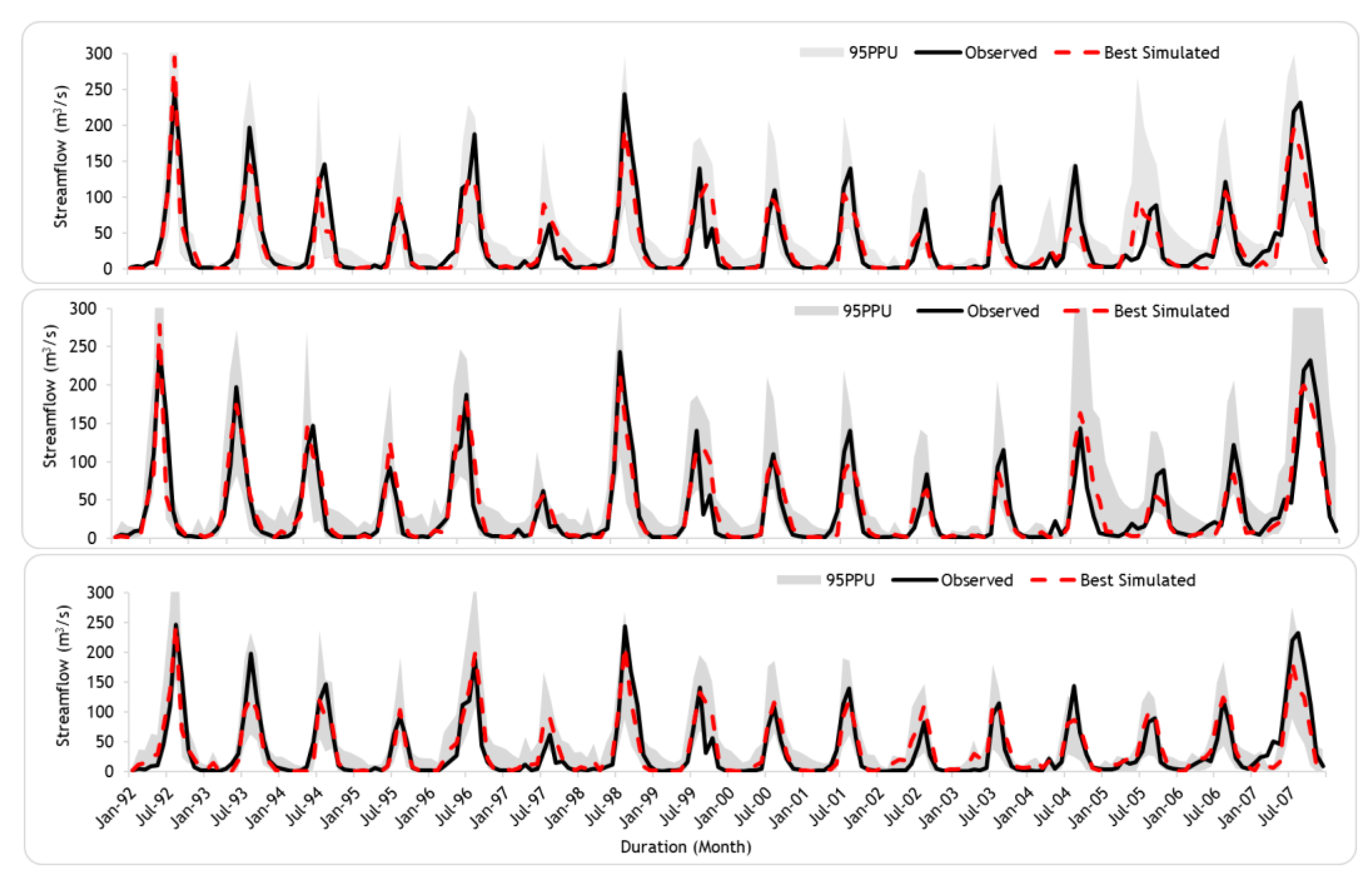
3.1. Hydrological Model Performance and Subbasin Discretization

The findings of the sensitivity analysis indicated (Table 1 and Figure 4) that the parameters ALPHA BNK, CN2, and GW DELAY were the most significant parameters in terms of the sensitivity levels in the majority of the discretization of each subbasin, Abelti, Wabi, and Gecha, respectively. Furthermore, CN2 is among the three most sensitive parameters in all the study watersheds. Because the parameter CN2 is crucial in determining how much runoff is generated from a hydrological response unit, the three watersheds’ streamflow models’ sensitivity to the parameter was anticipated [29,62].
Streamflow data for Abelti and Wabi (1992–2007) and Gecha (1996–2012) were used to assess the model’s simulation capabilities. The watershed calibration periods for Abelti, Wabi, and Gecha are (1992–2002), (1992–2001), and (1996–2009), respectively. Their separate validation periods were (2003–2007), (2002–2007), and (2010–2012). The values of the objective function (NSE) in Table 2 show how sensitive the model’s performance corresponds to the number of subbasin divisions and is used to replicate the observed hydrograph. The model’s parameters were adjusted for every discretization level of the subbasin in each watershed to assess how sensitive they were in the model. The Abelti watershed, the Wabi watershed, and the Gecha watershed all had subbasin subdivisions of 30, 3, and 3, respectively, which led to the best simulation results for the overall observed flow hydrograph. The coarser subdivision model typically performed poorly in the watersheds compared to its performance at a finer subbasin spatial scale. The implication of this finding is that datasets with spatial clarity are more reliable.

3.2. Impacts of Parameter Sampling Distribution on Subbasin Spatial Scale

The SUFI2 simulation employed 500 samples for sensitivity analysis. The first three most sensitive factors in each watershed’s subbasin spatial level are shown in scatter plots (Figure 5, Figure 6 and Figure 7). These examples correspond to well-known features. Figure 5, Figure 6 and Figure 7 provide dotty plots for the Abelti, Gecha, and Wabi watersheds at each subbasin spatial scale. The consequences of parameter ALPHA BNK are more noticeable in the Abelti watershed at all subbasin division stages, whereas GW DELAY and CN2 are more noticeable in the Gecha and Wabi watersheds, respectively. Additionally, high-density sample areas are shown on dotty plots with a density distribution. High- and relatively low-parameter sampling zones are shown by the dark and light blue dotty plots, respectively, while individual observations are indicated by the yellow symbols. The parameter samples are therefore somewhat concentrated mostly around the peak value across all watersheds for those subbasin subdivision levels, as evidenced by the dotty plots.

3.3. Parameter Uncertainty in Hydrological Modeling across Various Subbasin Spatial Scales

The 95PPU was calculated using the SUFI2 approach. Figure 8, Figure 9 and Figure 10 depict the measured and well-simulated streamflow patterns, as well as the 95PPU band. The P- and R-factors served as the model’s performance measures and were used to compute uncertainty. Hence, in this study, the metrics were determined using the uncertainty results for the Abelti watershed’s subbasin subdivision scales of 4, 8, and 30, the Gecha watershed’s subbasin subdivision scales of 3, 3, and 23, and the Wabi watershed’s subbasin subdivision scales of 3, 3, and 27. After employing the P-to-R-factor ratio (P/R), it was discovered that the parameter uncertainty results obtained using the SUFI2 approach for the Abelti, Gecha, and Wabi watersheds performed outstandingly at subbasin partition sizes of 8, 3, and 3, respectively [70]. Out of the whole basin area, the mean subbasin division that yields the lowest amount of uncertainty in the study is determined to be between 11% and 27%. The mean subbasin division for the optimal reproduced SWAT model’s simulated flow, on the other hand, was determined to be 2% to 10% of the entire drainage system for the watersheds.

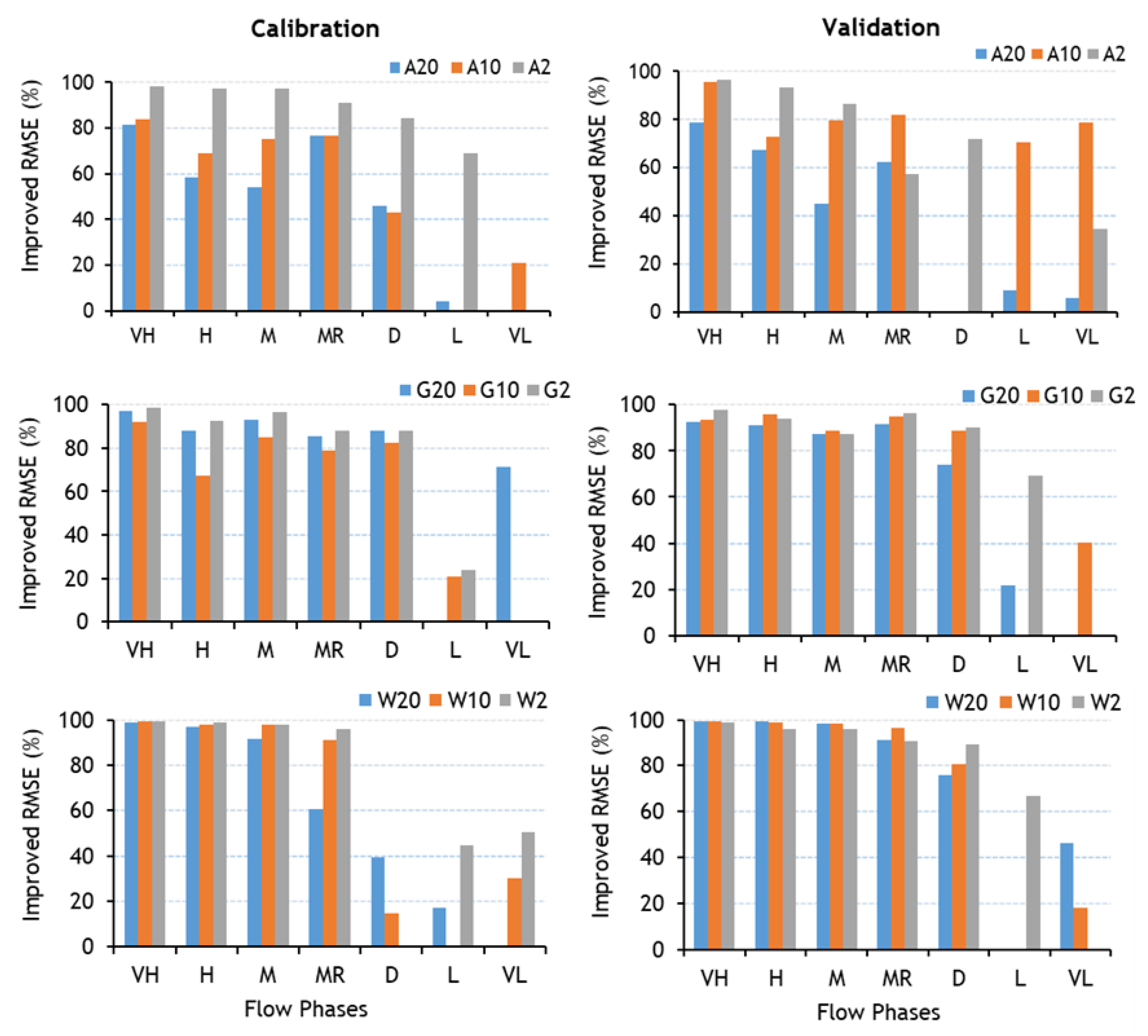
3.4. Impact of Subbasin Spatial Scales on the Reproduction of Various Flow Phases

The varied hydrograph phases must be accurately replicated for more efficient water management and planning. Different flow quantiles may be described using the flow duration curve (FDC). To more precisely determine the appropriate subbasin number of various views for each hydrograph plot in the study basins, the FDCs were then divided into seven quantiles. Figure 11 displays, for the Abelti, Wabi, and Gecha watersheds, the 95PPU plots of the best-estimated flows at various subbasin geographical sizes.
Performance varied slightly across the board since the simulation used varied subbasin geographic sizes. The modeling of these different flow phases also exhibits performance variances in the study case (see Figure 11).
The analysis shows that the absurdly inflated estimates of very-low, low, dry, and midrange flows were made at the lower subbasin partition scale for the Abelti catchment scenario. On the other hand, at the upper subbasin divisional levels, the extremely high flow was underestimated. The remaining high and moist flows, despite their appearing to be overstated, are actually fairly minor (see Figure 11). The SWAT model performed poorly in replicating the Abelti watershed’s dry and low flows throughout all subbasin spatial scales, as seen in Figure 11. The simulated flow variation, on the other hand, was extremely close to the observations, and it reproduced the moist, high, and very-high flows with good precision. Apart from the very high flows, the Abelti watershed SWAT model performance was found to reflect almost every flow regime across subbasin subdivisions 8 and 30. The findings could be explained by CN2’s low and high responsiveness at coarser and finer subbasin levels, respectively, because it has been demonstrated that CN2 has a considerable influence on the SWAT model [74].
Figure 12 depicts the improvements in RMSE for modeling the various flow phases in the analyzed watersheds over the periods of calibration and validation. The calibration phase had average RMSE advancements of 58%, 68%, and 63%, whereas its validation period showed average RMSE improvements of 56%, 71%, and 63%, respectively, at the Abelti, Gecha, and Wabi catchments’ different flow phases by using an appropriate subbasin geographic level.

4. Discussion

This study examines the impact of subbasin spatial scale on the hydrological model prediction uncertainty of exceptional stream flows. Thus, for the results of a specific basin to be valid, a hydrological model must operate successfully in line with the necessary statistical criteria.
A good estimate and knowledge of the behavior of the basin’s many runoff components are just as critical as a good overall model. In general, regardless of the degree of spatial discretization, the SWAT model captures the hydrological processes of the research basin utilizing the output of simulated hydrographs and obtained goodness-of-fit values [75]. However, the spatial discretization of subbasins is critical in recreating various simulated flow phases for the different quantile flows.
Similar to the work of [76], our results demonstrate that catchment size has no discernible influence on the sensitivity of a number of factors, such as CN2 and ALPHA_BNK. Another study, however, discovered that CN2 affects subbasin discretization, demonstrating that when subbasin discretization rises, CN2’s sensitivity rank also rises [11]. It is true that the classification underlying soil and land use usage for every subbasin may vary when the subbasin subdivision level changes, which may therefore have an impact on CN2. The outcome matches the results of [11,77], who both concluded that CN2 is a crucial variable affecting hydrological simulations in all model applications. The largest source of uncertainty in streamflow simulations, according to some studies, was CN2 [78,79]. The fact that the relevance of the SWAT model parameters changed with the number of subbasins demonstrated the influence of subbasin partitioning on parameter responsiveness.
These results are in line with those reported by [24,80], who discovered that increasing the amount of subbasin discretization boosted simulation accuracy. The precision of the model plateaus at the subdivision level of the subbasin correlates to the highest accuracy. The 30 (Abelti), 3 (Wabi), and 3 (Gecha) subbasin subdivision schemes accurately reflect the spatial variations in spatio-climatic conditions, which might provide an explanation for the performance variance as being linked to CN2’s sensitivity to the subbasin spatial scale. The overall flow domain simulation experiments for each level of subbasin segmentation were good, as stated by [81], with an NSE value above 0.65.
It is crucial to bear in mind that when the NSE value is more than 0.5, the scores of the flow simulation of the hydrological model are acceptable [81]. Figure 5, Figure 6 and Figure 7 show that the NSE values for the majority of sampling locations in the study watersheds were more than 0.5. Contrary to Figure 7, which displays all sample locations in the Wabi watershed with NSE values above 0.5, the scatter diagrams for the Abelti and Gecha watersheds also include some sampling frequencies with NSE values less than 0.5.
Information on measured flow and precipitation data may be the main issue in the Abelti and Gecha basins, respectively. Data on rainfall from the watershed’s insufficient geographic coverage might possibly be a factor. Aside from the fact that the parameter sampling in all three catchments was insufficient, the results demonstrate that larger sampling sets would be better for locations with limited data to increase the replicability of the sample points.
Our findings show that subbasin geographic size has little influence on the evaluation of uncertainty in hydrological model parameters, with the fairly coarse subbasin geographical size having the lowest uncertainty compared to the smaller subbasin division levels. It thus demonstrates how combining meteorological and physical variables at a finer geographical dimension might help to reduce uncertainty in hydrological model parameters related to watershed data quality. The conclusions of this study agree with those of [11]. The main challenge in the Abelti and Gecha basins may be connected to the recorded flow and precipitation data. Precipitation data from the watershed’s limited geographic coverage might be a concern. Aside from the fact that parameter sampling was insufficient in all three catchments, the results demonstrate that larger sampling sets would be better for areas with low data to increase the reliability and accuracy of the sample points.
The 95PPU contained more than 70% of the observations in the lower subbasin subdivision levels 4 and 8 of the Abelti watershed, as well as the entire subbasin division units in the Gecha and Wabi watersheds. However, as the quantity of drainage basins grew, so did the relative thickness of the 95PPU. The fact that all the P- and R-factor values were within acceptable ranges suggests that all the parameter uncertainties were maintained within acceptable limitations. As a result, the 95PPU bracketed the lion’s share of the observed values, confirming SWAT’s ability to model flow dynamics within the watershed under discussion. It was discovered that the Abelti and Gecha watersheds have wider relative 95PPUs than the Wabi watershed. This may be because the precision with which the injected values with the watersheds of Abelti and Gecha strongly influence the quality of hydrological model simulation, creating a high degree of uncertainty in the results. The Abelti and Gecha watersheds have few and erratically placed weather gauging stations.
Despite being recreated with more accuracy at smaller subdivisions, the best-simulated low flow response on the larger subbasin spatial scale deviated significantly from the real values (Figure 8 and Figure 10). The Gecha watershed’s data quality may be a contributing factor in the absence of solid evidence for spatial diversity impacts (Figure 9).
Replicating very low and low flows across the Wabi watershed fared better at smaller to intermediate subbasin sizes (subbasin divisions of 3 and 27). However, at a modest to wider spatial scale, the SWAT output recreated the features of the very high, high, moist, and dry observed flows quite consistently. The model effectively duplicated the bulk of the flows on a medium spatial scale.
In certain circumstances, the mid-range and dry flow exceed the expected flow at smaller spatial scales. However, other components present throughout the model simulation process might be the source of the variance. The Gecha watershed’s very low, low, dry, and midrange flows might be more properly approximated at a reduced geographical scale. However, the model’s output at a broader geographical scale accurately represented the response variables of very high, high, and moist observed flows. As a consequence, the results show that improved replication of the low flow unique phases should be attainable with a chance of 40–100% utilizing lower geographical scales, which increase the number of drainage basins identified during the definition of the SWAT watershed. This conclusion is consistent with the findings of comparable studies, including (e.g., [11]). As a result, the findings of this study may be beneficial for distributed model water quality and quantity modeling at an appropriate subbasin spatial scale.
Figure 11 clearly shows that the 95PPU comparative ranges for very high flows are narrower than those for low flows. Given that the majority of hydrological models are designed to replicate peak flows and that the NSE performance metric was used to fine-tune the model’s parameters, which obviously favor the replication of high flows, this conclusion is unsurprising. The 95PPU covered the observations in the high-flow region with a coverage of more than 100% compared to the flow ranges. It is obvious that the strategy employed in this work, which comprises looking at the correct subbasin varied sizes to every flow stage of the FDC, appears to be well adapted to decreasing the discrepancy between hydrological model findings and observations. More study is suggested to increase the precision of the low-flow hydrological model parameters.
The contrast in the spatial scale of the subbasin is noticeable when compared to the reproduction of the individual flow phases throughout the whole recorded hydrograph. With more subbasin subdivisions, there is less variation in the produced outcomes, and the conclusions may be more consistent. Figure 11 depicts in great detail how the spatial presentations of the model’s physical and meteorological inputs, as well as the circumstances for watershed management, all have an effect on the disparities in the modeling output processes. The simulation’s inaccuracy was nearly twice as high in the Abelti and Gecha watersheds, as it was notably in low flow regimes in the Wabi watershed.
The improvement of RMSE for investigating the optimal subbasin spatial scale throughout the calibration period was 81% when simulating mid-range flow in the Abelti watershed, 86% when modeling dry flow in the Gecha watershed, and 27% when simulating very low flow in the Wabi watershed. During the validation period, the Abelti watershed’s very low flow was recreated with a 40% accuracy gain, the Gecha watershed’s dry flow with an 84% accuracy gain, and the Wabi watershed’s dry flow with an 81% accuracy gain. This is obvious from the approach of the study, which was demonstrated to be an effective strategy for minimizing SWAT simulation error while simulating low flows.

5. Conclusions

The primary sources of error in hydrologic simulation are closely associated with physical data input, model parameters, and the structure of the model. In this work, SUFI2 was applied to characterize parameter uncertainty using SWAT modeling. Moreover, the subbasin spatial scale effects on the SWAT modeling prediction uncertainty were investigated. To replicate various flow phases of the FDC for the Abelti, Gecha, and Wabi watersheds in the Omo-Gibe River Basin, Ethiopia, the uncertainty of the hydrological modeling parameter was assessed. The Wabi watershed seems to have a reasonable spatial inclusiveness of meteorological and physical data input, in contrast to the Abelti and Gecha watersheds, which have rather poor spatial representations of these inputs to the hydrological model. Thus, this study also considered how the precision of the data input and the conditions for watershed management affect the variability in the uncertainty in the hydrological modeling parameters. The analysis revealed that the subbasin spatial scale substantially affected the reproduction of various flow phases but only slightly affected the overall flow simulations.
The 95PPU covered the majority of the observed hydrograph with the coarser geographic scale of the subbasin. Moreover, the coarser subbasin geographic size resulted in a smaller 95PPU proportional width. The key findings of the study are summarized as follows: (1) for the Abelti, Gecha, and Wabi watersheds, SWAT was able to reproduce the observed hydrograph with more than 85%, 73%, and 82% accuracy in terms of NSE, respectively; (2) the SWAT model performed much better in recreating moist, high, and very-high flows than it did in replicating dry, low, and very-low flows in the watersheds. This out-come is in line with previous studies [e.g., 11]. Moreover, with low flows compared to high flows, the relative uncertainty range widens; (3) The establishment of proper subbasin spatial scale considerably improved hydrologic modeling accuracy in mimicking the FDC’s various flow phases. As a result, in order to better understand the severity and frequency of these diverse phases of flow behavior, a variety of relevant subbasin spatial scales may be required (e.g., for flood damage estimates and water quality models); (4) in the Abelti, Gecha, and Wabi watersheds, the mean RMSE improvements in subbasin spatial scales for high flows varied by 79%, 91%, and 98%, respectively, whereas those for low flows varied similarly by 29%, 42%, and 32%. Consequently, a smaller subbasin spatial scale (towards to distributed model) may better replicate low flows, while a larger subbasin spatial scale (towards to lumped model) enhances high flow replication precision. The subbasin spatial scales used in this study may have adequately captured the spatial variability in the physical and climatic aspects of the watersheds. It is critical to remember that the physical and climatic parameters of the watershed analyzed may change spatially, which may have an impact on the conclusions made. Hence, further investigation on similar subbasin spatial scales across other watersheds is needed.
Given the nature of the study, combining morphological and meteorological inputs at a larger spatial scale within a subbasin can often lower the uncertainty of the hydrological model parameters. However, compared to the larger subbasin spatial scales, the simulation’s best results were produced at the smaller subbasin spatial scale and were more consistent with the data that had actually been observed. Most of the observed high flows were contained by the 95PPU, but a large percentage of the recorded low flows was not. Therefore, more work must be put into lowering the parameter uncertainty in low-flow hydrologic modeling.
Last but not least, the research significantly increased the hydrological model’s accuracy in simulating the different flow phases by using a reasonable subbasin spatial scale; for the Abelti, Gecha, and Wabi watersheds, the overall average simulation errors were decreased by roughly 82, 79, and 77%, respectively. Therefore, the suggested method could help us better comprehend the frequency and size of the various flow quantiles for a reasonable assessment of high flows (for example, reducing flood risks) and low flows (for example, modeling water quality).

Author Contributions

Preparation of a first draft of a written report, as well as the design, methodology, interpretation, and study of the research, B.M.G.; the work was evaluated and revised, and the conclusions were monitored and validated by A.M.M., A.K.J. and G.T. After reading the manuscript, all contributors agreed on its published version. All authors have read and agreed to the published version of the manuscript.

Funding

This research received no external funding.

Data Availability Statement

Not applicable.

Acknowledgments

The data used in this study were gathered from the Water and Land Resources Center (WLRC), the National Meteorology Agency of Ethiopia (NMA), and the Ethiopian Ministry of Water and Energy (MWE).

Conflicts of Interest

The authors declare no conflict of interest.

References

  1. Kibuye, F.A.; Gall, H.E.; Veith, T.L.; Elkin, K.R.; Elliott, H.A.; Harper, J.P.; Watson, J.E. Influence of hydrologic and anthropogenic drivers on emerging organic contaminants in drinking water sources in the Susquehanna River Basin. Chemosphere 2020, 245, 125583. [Google Scholar] [CrossRef] [PubMed]
  2. Arnold, J.G.; Moriasi, D.N.; Gassman, P.W.; Abbaspour, K.C.; White, M.J.; Srinivasan, R.; Santhi, C.; Harmel, R.; Van Griensven, A.; Van Liew, M.W. SWAT: Model use, calibration, and validation. Trans. ASABE 2012, 55, 1491–1508. [Google Scholar] [CrossRef]
  3. Butts, M.B.; Payne, J.T.; Kristensen, M.; Madsen, H. An evaluation of the impact of model structure on hydrological modelling uncertainty for streamflow simulation. J. Hydrol. 2004, 298, 242–266. [Google Scholar] [CrossRef]
  4. Devia, G.K.; Ganasri, B.P.; Dwarakish, G.S. A review on hydrological models. Aquat. Procedia 2015, 4, 1001–1007. [Google Scholar] [CrossRef]
  5. Gao, H.; Tang, Q.; Shi, X.; Zhu, C.; Bohn, T.; Su, F.; Pan, M.; Sheffield, J.; Lettenmaier, D.; Wood, E. Water budget record from Variable Infiltration Capacity (VIC) model. In Algorithm Theoretical Basis Document for Terrestrial Water Cycle Data Records; 2010; Available online: https://www.researchgate.net/publication/268367169_Water_Budget_Record_from_Variable_Infiltration_Capacity_VIC_Model (accessed on 28 November 2022).
  6. Pandi, D.; Kothandaraman, S.; Kuppusamy, M. Hydrological models: A review. Int. J. Hydrol. Sci. Technol. 2021, 12, 223–242. [Google Scholar] [CrossRef]
  7. Refsgaard, J.C. Parameterisation, calibration and validation of distributed hydrological models. J. Hydrol. 1997, 198, 69–97. [Google Scholar] [CrossRef]
  8. Carpenter, T.M.; Georgakakos, K.P. Intercomparison of lumped versus distributed hydrologic model ensemble simulations on operational forecast scales. J. Hydrol. 2006, 329, 174–185. [Google Scholar] [CrossRef]
  9. Dal Molin, M.; Schirmer, M.; Zappa, M.; Fenicia, F. Understanding dominant controls on streamflow spatial variability to set up a semi-distributed hydrological model: The case study of the Thur catchment. Hydrol. Earth Syst. Sci. 2020, 24, 1319–1345. [Google Scholar] [CrossRef] [Green Version]
  10. Veettil, A.V.; Green, T.R.; Kipka, H.; Arabi, M.; Lighthart, N.; Mankin, K.; Clary, J. Fully distributed versus semi-distributed process simulation of a highly managed watershed with mixed land use and irrigation return flow. Environ. Model. Softw. 2021, 140, 105000. [Google Scholar] [CrossRef]
  11. Tegegne, G.; Kim, Y.-O.; Seo, S.B.; Kim, Y. Hydrological modelling uncertainty analysis for different flow quantiles: A case study in two hydro-geographically different watersheds. Hydrol. Sci. J. 2019, 64, 473–489. [Google Scholar] [CrossRef]
  12. Abbaspour, K.C. SWAT-CUP: SWAT calibration and uncertainty programs—A user manual. Eawag. Dübendorf. Switz. 2015, 16–70. [Google Scholar]
  13. Beven, K. Prophecy, reality and uncertainty in distributed hydrological modelling. Adv. Water Resour. 1993, 16, 41–51. [Google Scholar] [CrossRef]
  14. Faramarzi, M.; Abbaspour, K.C.; Vaghefi, S.A.; Farzaneh, M.R.; Zehnder, A.J.; Srinivasan, R.; Yang, H. Modeling impacts of climate change on freshwater availability in Africa. J. Hydrol. 2013, 480, 85–101. [Google Scholar] [CrossRef]
  15. Rozos, E.; Dimitriadis, P.; Bellos, V. Machine Learning in Assessing the Performance of Hydrological Models. Hydrology 2021, 9, 5. [Google Scholar] [CrossRef]
  16. Abdar, M.; Pourpanah, F.; Hussain, S.; Rezazadegan, D.; Liu, L.; Ghavamzadeh, M.; Fieguth, P.; Cao, X.; Khosravi, A.; Acharya, U.R. A review of uncertainty quantification in deep learning: Techniques, applications and challenges. Inf. Fusion 2021, 76, 243–297. [Google Scholar] [CrossRef]
  17. McMillan, H.K.; Westerberg, I.K.; Krueger, T. Hydrological data uncertainty and its implications. Wiley Interdiscip. Rev. Water 2018, 5, e1319. [Google Scholar] [CrossRef] [Green Version]
  18. Arnold, J.G.; Srinivasan, R.; Muttiah, R.S.; Williams, J.R. Large area hydrologic modeling and assessment part I: Model development. JAWRA J. Am. Water Resour. Assoc. 1998, 34, 73–89. [Google Scholar] [CrossRef]
  19. Blöschl, G.; Sivapalan, M. Scale issues in hydrological modelling: A review. Hydrol. Process. 1995, 9, 251–290. [Google Scholar] [CrossRef]
  20. Craig, J.R.; Brown, G.; Chlumsky, R.; Jenkinson, R.W.; Jost, G.; Lee, K.; Mai, J.; Serrer, M.; Sgro, N.; Shafii, M. Flexible watershed simulation with the Raven hydrological modelling framework. Environ. Model. Softw. 2020, 129, 104728. [Google Scholar] [CrossRef]
  21. Kling, H.; Gupta, H. On the development of regionalization relationships for lumped watershed models: The impact of ignoring sub-basin scale variability. J. Hydrol. 2009, 373, 337–351. [Google Scholar] [CrossRef]
  22. Tan, M.L.; Gassman, P.W.; Yang, X.; Haywood, J. A review of SWAT applications, performance and future needs for simulation of hydro-climatic extremes. Adv. Water Resour. 2020, 143, 103662. [Google Scholar] [CrossRef]
  23. Wood, E.F.; Sivapalan, M.; Beven, K.; Band, L. Effects of spatial variability and scale with implications to hydrologic modeling. J. Hydrol. 1988, 102, 29–47. [Google Scholar] [CrossRef]
  24. Mamillapalli, S.; Srinivasan, R.; Arnold, J.; Engel, B.A. Effect of spatial variability on basin scale modeling. In Proceedings of the Third International Conference/Workshop on Integrating GIS and Environmental Modeling, Santa Fe, NM, USA, 21–25 January 1996. [Google Scholar]
  25. Bingner, R.; Garbrecht, J.; Arnold, J.G.; Srinivasan, R. Effect of Watershed Subdivision on Simulation Runoff and Fine Sediment Yield. Trans. ASAE 1997, 40, 1329–1335. [Google Scholar] [CrossRef]
  26. Kumar, S.; Merwade, V. Impact of watershed subdivision and soil data resolution on SWAT model calibration and parameter uncertainty. JAWRA J. Am. Water Resour. Assoc. 2009, 45, 1179–1196. [Google Scholar] [CrossRef]
  27. Tianqi, A.; Yoshitani, J.; Takeuchi, K.; Fukami, K. Effects of sub-basin scale on runoff simulation in distributed hydrological model: BTOPMC. In Weather Radar Information and Distributed Hydrological Modelling, Proceedings of the International Symposium (Symposium HS03) Held During IUGG 2003, the XXIII General Assembly of the International Union of Geodesy and Geophysics, Sapporo, Japan, 30 June–11 July 2003; International Association of Hydrological Sciences: Wallingford, UK, 2003; p. 227. [Google Scholar]
  28. Hamby, D.M. A review of techniques for parameter sensitivity analysis of environmental models. Environ. Monit. Assess. 1994, 32, 135–154. [Google Scholar] [CrossRef]
  29. Tegegne, G.; Kim, Y.-O. Modelling ungauged catchments using the catchment runoff response similarity. J. Hydrol. 2018, 564, 452–466. [Google Scholar] [CrossRef]
  30. Abbaspour, K.C.; Yang, J.; Maximov, I.; Siber, R.; Bogner, K.; Mieleitner, J.; Zobrist, J.; Srinivasan, R. Modelling hydrology and water quality in the pre-alpine/alpine Thur watershed using SWAT. J. Hydrol. 2007, 333, 413–430. [Google Scholar] [CrossRef]
  31. Coxon, G.; Freer, J.; Westerberg, I.K.; Wagener, T.; Woods, R.; Smith, P. A novel framework for discharge uncertainty quantification applied to 500 UK gauging stations. Water Resour. Res. 2015, 51, 5531–5546. [Google Scholar] [CrossRef] [Green Version]
  32. Dwelle, M.C.; Kim, J.; Sargsyan, K.; Ivanov, V.Y. Streamflow, stomata, and soil pits: Sources of inference for complex models with fast, robust uncertainty quantification. Adv. Water Resour. 2019, 125, 13–31. [Google Scholar] [CrossRef]
  33. Fan, Y. Uncertainty quantification in hydrologic predictions: A brief review. J. Environ. Inform. Lett. 2019, 2, 48–56. [Google Scholar] [CrossRef] [Green Version]
  34. Mannina, G.; Viviani, G. An urban drainage stormwater quality model: Model development and uncertainty quantification. J. Hydrol. 2010, 381, 248–265. [Google Scholar] [CrossRef]
  35. Smith, R.C. Uncertainty Quantification: Theory, Implementation, and Applications; SIAM: Philadelphia, PA, USA, 2013; Volume 12. [Google Scholar]
  36. Uniyal, B.; Jha, M.K.; Verma, A.K. Parameter identification and uncertainty analysis for simulating streamflow in a river basin of Eastern India. Hydrol. Process. 2015, 29, 3744–3766. [Google Scholar] [CrossRef]
  37. Valdez, E.S.; Anctil, F.; Ramos, M.-H. Choosing between post-processing precipitation forecasts or chaining several uncertainty quantification tools in hydrological forecasting systems. Hydrol. Earth Syst. Sci. 2022, 26, 197–220. [Google Scholar] [CrossRef]
  38. Wang, C.; Duan, Q.; Tong, C.H.; Di, Z.; Gong, W. A GUI platform for uncertainty quantification of complex dynamical models. Environ. Model. Softw. 2016, 76, 1–12. [Google Scholar] [CrossRef] [Green Version]
  39. Wang, H.; Wang, C.; Wang, Y.; Gao, X.; Yu, C. Bayesian forecasting and uncertainty quantifying of stream flows using Metropolis–Hastings Markov Chain Monte Carlo algorithm. J. Hydrol. 2017, 549, 476–483. [Google Scholar] [CrossRef] [Green Version]
  40. Abbaspour, K.C.; Johnson, C.; Van Genuchten, M.T. Estimating uncertain flow and transport parameters using a sequential uncertainty fitting procedure. Vadose Zone J. 2004, 3, 1340–1352. [Google Scholar] [CrossRef]
  41. Beven, K.; Binley, A. The future of distributed models: Model calibration and uncertainty prediction. Hydrol. Process. 1992, 6, 279–298. [Google Scholar] [CrossRef]
  42. Sorenson, H.W.; Alspach, D.L. Recursive Bayesian estimation using Gaussian sums. Automatica 1971, 7, 465–479. [Google Scholar] [CrossRef]
  43. Xiu, D.; Karniadakis, G.E. Modeling uncertainty in flow simulations via generalized polynomial chaos. J. Comput. Phys. 2003, 187, 137–167. [Google Scholar] [CrossRef]
  44. Vrugt, J.A.; Gupta, H.V.; Bouten, W.; Sorooshian, S. A Shuffled Complex Evolution Metropolis algorithm for optimization and uncertainty assessment of hydrologic model parameters. Water Resour. Res. 2003, 39, 1201. [Google Scholar] [CrossRef] [Green Version]
  45. Vrugt, J.A.; Diks, C.G.; Gupta, H.V.; Bouten, W.; Verstraten, J.M. Improved treatment of uncertainty in hydrologic modeling: Combining the strengths of global optimization and data assimilation. Water Resour. Res. 2005, 41, W01017. [Google Scholar] [CrossRef]
  46. Moges, E.; Demissie, Y.; Larsen, L.; Yassin, F. Review: Sources of Hydrological Model Uncertainties and Advances in Their Analysis. Water 2021, 13, 28. [Google Scholar] [CrossRef]
  47. Awulachew, S.B.; Yilma, A.D.; Loulseged, M.; Loiskandl, W.; Ayana, M.; Alamirew, T. Water Resources and Irrigation Development in Ethiopia; IWMI: Colombo, Sri Lanka, 2007; Volume 123. [Google Scholar]
  48. Neitsch, S.L.; Arnold, J.G.; Kiniry, J.R.; Williams, J.R. Soil and Water Assessment Tool Theoretical Documentation Version 2009; Texas Water Resources Institute: College Station, TX, USA, 2011. [Google Scholar]
  49. Chaemiso, S.E.; Abebe, A.; Pingale, S.M. Assessment of the impact of climate change on surface hydrological processes using SWAT: A case study of Omo-Gibe river basin, Ethiopia. Model. Earth Syst. Environ. 2016, 2, 1–15. [Google Scholar] [CrossRef] [Green Version]
  50. Hussainzada, W.; Lee, H.S. Hydrological modelling for water resource management in a semi-arid mountainous region using the soil and water assessment tool: A case study in northern Afghanistan. Hydrology 2021, 8, 16. [Google Scholar] [CrossRef]
  51. Jiang, L.; Zhu, J.; Chen, W.; Hu, Y.; Yao, J.; Yu, S.; Jia, G.; He, X.; Wang, A. Identification of Suitable Hydrologic Response Unit Thresholds for Soil and Water Assessment Tool Streamflow Modelling. Chin. Geogr. Sci. 2021, 31, 696–710. [Google Scholar] [CrossRef]
  52. Nguyen, T.V.; Dietrich, J.; Dang, T.D.; Tran, D.A.; Van Doan, B.; Sarrazin, F.J.; Abbaspour, K.; Srinivasan, R. An interactive graphical interface tool for parameter calibration, sensitivity analysis, uncertainty analysis, and visualization for the Soil and Water Assessment Tool. Environ. Model. Softw. 2022, 156, 105497. [Google Scholar] [CrossRef]
  53. Ullrich, A.; Volk, M. Application of the Soil and Water Assessment Tool (SWAT) to predict the impact of alternative management practices on water quality and quantity. Agric. Water Manag. 2009, 96, 1207–1217. [Google Scholar] [CrossRef]
  54. Nesru, M.; Shetty, A.; Nagaraj, M. Multi-variable calibration of hydrological model in the upper Omo-Gibe basin, Ethiopia. Acta Geophys. 2020, 68, 537–551. [Google Scholar] [CrossRef]
  55. Beven, K. Changing ideas in hydrology—The case of physically-based models. J. Hydrol. 1989, 105, 157–172. [Google Scholar] [CrossRef]
  56. Pokhrel, P.; Gupta, H.; Wagener, T. A spatial regularization approach to parameter estimation for a distributed watershed model. Water Resour. Res. 2008, 44, W12419. [Google Scholar] [CrossRef]
  57. Seibert, J.; Staudinger, M.; Meerveld, H. Validation and over-parameterization—Experiences from hydrological modeling. In Computer Simulation Validation; Springer: Cham, Switzerland, 2019; pp. 811–834. [Google Scholar]
  58. Malik, M.A.; Dar, A.Q.; Jain, M.K. Modelling streamflow using the SWAT model and multi-site calibration utilizing SUFI-2 of SWAT-CUP model for high altitude catchments, NW Himalaya’s. Model. Earth Syst. Environ. 2022, 8, 1203–1213. [Google Scholar] [CrossRef]
  59. Song, X.; Zhang, J.; Zhan, C.; Xuan, Y.; Ye, M.; Xu, C. Global sensitivity analysis in hydrological modeling: Review of concepts, methods, theoretical framework, and applications. J. Hydrol. 2015, 523, 739–757. [Google Scholar] [CrossRef] [Green Version]
  60. Yang, X.; Jomaa, S.; Rode, M. Spatiotemporally distributed sensitivity analysis for catchment water quality models. Geophys. Res. Abstr. 2019, 21, 1. [Google Scholar]
  61. Abbaspour, K.C.; Vaghefi, S.A.; Srinivasan, R. A guideline for successful calibration and uncertainty analysis for soil and water assessment: A review of papers from the 2016 international SWAT conference. Water 2017, 10, 6. [Google Scholar] [CrossRef] [Green Version]
  62. Cibin, R.; Sudheer, K.; Chaubey, I. Sensitivity and identifiability of stream flow generation parameters of the SWAT model. Hydrol. Process. Int. J. 2010, 24, 1133–1148. [Google Scholar] [CrossRef]
  63. Dakhlalla, A.O.; Parajuli, P.B. Assessing model parameters sensitivity and uncertainty of streamflow, sediment, and nutrient transport using SWAT. Inf. Process. Agric. 2019, 6, 61–72. [Google Scholar] [CrossRef]
  64. Narsimlu, B.; Gosain, A.K.; Chahar, B.R.; Singh, S.K.; Srivastava, P.K. SWAT model calibration and uncertainty analysis for streamflow prediction in the Kunwari River Basin, India, using sequential uncertainty fitting. Environ. Process. 2015, 2, 79–95. [Google Scholar] [CrossRef]
  65. Spruill, C.A.; Workman, S.R.; Taraba, J.L. Simulation of daily and monthly stream discharge from small watersheds using the SWAT model. Trans. ASAE 2000, 43, 1431. [Google Scholar] [CrossRef]
  66. Gupta, H.V.; Kling, H.; Yilmaz, K.K.; Martinez, G.F. Decomposition of the mean squared error and NSE performance criteria: Implications for improving hydrological modelling. J. Hydrol. 2009, 377, 80–91. [Google Scholar] [CrossRef] [Green Version]
  67. Hosseini, S.H.; Khaleghi, M.R. Application of SWAT model and SWAT-CUP software in simulation and analysis of sediment uncertainty in arid and semi-arid watersheds (case study: The Zoshk–Abardeh watershed). Model. Earth Syst. Environ. 2020, 6, 2003–2013. [Google Scholar] [CrossRef]
  68. Khalid, K.; Ali, M.F.; Abd Rahman, N.F.; Mispan, M.R.; Haron, S.H.; Othman, Z.; Bachok, M.F. Sensitivity analysis in watershed model using SUFI-2 algorithm. Procedia Eng. 2016, 162, 441–447. [Google Scholar] [CrossRef] [Green Version]
  69. Nash, J.E.; Sutcliffe, J.V. River flow forecasting through conceptual models part I—A discussion of principles. J. Hydrol. 1970, 10, 282–290. [Google Scholar] [CrossRef]
  70. Abbaspour, K.C.; Rouholahnejad, E.; Vaghefi, S.; Srinivasan, R.; Yang, H.; Kløve, B. A continental-scale hydrology and water quality model for Europe: Calibration and uncertainty of a high-resolution large-scale SWAT model. J. Hydrol. 2015, 524, 733–752. [Google Scholar] [CrossRef] [Green Version]
  71. Kannan, N.; Jeong, J. An approach for estimating stream health using flow duration curves and indices of hydrologic alteration. EPA Reg. 2011, 6. [Google Scholar]
  72. Pfannerstill, M.; Guse, B.; Fohrer, N. Smart low flow signature metrics for an improved overall performance evaluation of hydrological models. J. Hydrol. 2014, 510, 447–458. [Google Scholar] [CrossRef]
  73. Yilmaz, K.K.; Gupta, H.V.; Wagener, T. A process-based diagnostic approach to model evaluation: Application to the NWS distributed hydrologic model. Water Resour. Res. 2008, 44, W09417. [Google Scholar] [CrossRef] [Green Version]
  74. Wu, L.; Liu, X.; Chen, J.; Yu, Y.; Ma, X. Overcoming equifinality: Time-varying analysis of sensitivity and identifiability of SWAT runoff and sediment parameters in an arid and semiarid watershed. Environ. Sci. Pollut. Res. 2022, 29, 31631–31645. [Google Scholar] [CrossRef]
  75. Caldeira, T.L.; Mello, C.R.; Beskow, S.; Timm, L.C.; Viola, M.R. LASH hydrological model: An analysis focused on spatial discretization. Catena 2019, 173, 183–193. [Google Scholar] [CrossRef]
  76. Singh, A.; Jha, S.K. Identification of sensitive parameters in daily and monthly hydrological simulations in small to large catchments in Central India. J. Hydrol. 2021, 601, 126632. [Google Scholar] [CrossRef]
  77. Gassman, P.W.; Reyes, M.R.; Green, C.H.; Arnold, J.G. The soil and water assessment tool: Historical development, applications, and future research directions. Trans. ASABE 2007, 50, 1211–1250. [Google Scholar] [CrossRef] [Green Version]
  78. Eckhardt, K.; Arnold, J. Automatic calibration of a distributed catchment model. J. Hydrol. 2001, 251, 103–109. [Google Scholar] [CrossRef]
  79. Guo, J.; Su, X. Parameter sensitivity analysis of SWAT model for streamflow simulation with multisource precipitation datasets. Hydrol. Res. 2019, 50, 861–877. [Google Scholar] [CrossRef] [Green Version]
  80. Haverkamp, S.; Srinivasan, R.; Frede, H.; Santhi, C. Subwatershed spatial analysis tool: Discretization of a distributed hydrologic model by statistical criteria. JAWRA J. Am. Water Resour. Assoc. 2002, 38, 1723–1733. [Google Scholar] [CrossRef]
  81. Moriasi, D.N.; Arnold, J.G.; Van Liew, M.W.; Bingner, R.L.; Harmel, R.D.; Veith, T.L. Model evaluation guidelines for systematic quantification of accuracy in watershed simulations. Trans. ASABE 2007, 50, 885–900. [Google Scholar] [CrossRef]
Figure 1. The study area: Abelti, Wabi and Gecha watersheds located in the Omo-Gibe River Basin, Ethiopia.
Remotesensing 15 00611 g001
Figure 2. Three subbasin subdivision levels for the study area (Abelti, Gecha and Wabi watersheds). (Note: A = watershed area).
Remotesensing 15 00611 g002
Figure 3. Variations in subbasin area and its subdivisions within the studied area.
Remotesensing 15 00611 g003
Figure 4. Sensitivity rank variation of the SWAT model’s flow parameters for the three subbasins of Abelti, Wabi, and Gecha, as determined by the t statistic, are shown on the left, center, and right, respectively.
Remotesensing 15 00611 g004
Figure 5. Dotty plots of the coefficient of NSE against SWAT parameters (left columns represent the most sensitive) using SUFI2 based on 500 samples from the Abelti watershed. (Note that # Subbasins 30, 8, and 4 account for 2%, 10%, and 20% of the Abelti watershed area, respectively.).
Remotesensing 15 00611 g005
Figure 6. Dotty plots of the coefficient of NSE against SWAT parameters (left columns represent the most sensitive) using SUFI2 based on 500 samples from the Gecha watershed. (Note that # Subbasins 23, 3, and 3 account for 2%, 10%, and 20% of the Gecha watershed area, respectively.).
Remotesensing 15 00611 g006
Figure 7. Dotty plots of the coefficient of NSE against SWAT parameters (left columns represent the most sensitive) using SUFI2 based on 500 samples from the Wabi watershed. (Note that # Subbasins 27, 3, and 3 account for 2%, 10%, and 20% of the Wabi watershed area, respectively.).
Remotesensing 15 00611 g007
Figure 8. Top-down orientation of observed and best-simulated flows with their 95% confidence level of the subbasin segmentations of 4, 8, and 30, respectively, at the Abelti watershed.
Remotesensing 15 00611 g008
Figure 9. Top-down orientation of observed and best-simulated flows with their 95% confidence level of the subbasin segmentations of 3, 3, and 23, respectively, at the Gecha watershed.
Remotesensing 15 00611 g009
Figure 10. Top-down orientation of observed and best-simulated flows with their 95% confidence level of subbasin segmentations 3, 3, and 27 in the Wabi watershed.
Remotesensing 15 00611 g010
Figure 11. Observed and best-simulated flow for the two extreme (0–5 and 95–100%) flow phases based on the 95PPU plot and several subbasin spatial scales of the Abelti, Wabi, and Gecha catchments (top-to-down, respectively). (Note that A = Abelti, G = Gecha, and W = Wabi together with their 2, 10, and 20 as percentages of the total area to obtain different subbasin numbers).
Remotesensing 15 00611 g011
Figure 12. Variations in the improved RMSE (%) at various flow phases for calibration and validation conditions (top-down orientation Abelti, Gecha and Wabi watersheds). Note: A = Abelti, G = Gecha, and W = Wabi watersheds 2, 10 and 20 = Percentage of total area for each watershed to obtain various subbasin divisions VL, L, D, MR, M, H, and VH represent very low, low, dry, midrange, moist, high, and very high, respectively.
Remotesensing 15 00611 g012
Table 1. SWAT model flow parameters used in the study basin.
Parameter Name with Their ExtensionParameter DescriptionsUnitValid Ranges
ALPHA_BF.gwBaseflow alpha factor(days)0–1
ALPHA_BNK.rteBaseflow alpha factor for bank storage(-)0–1
CH_K2.rteEffective hydraulic conductivity in main channel(mm/h)−0.01–500
CH_N2.rteManning’s “n” value for the main channel(-)−0.01–0.3
CN2.mgt (r)SCS runoff curve number(-)−0.2–0.2
ESCO.hruSoil evaporation compensation factor(-)0–1
GW_DELAY.gwGroundwater delay time(days)0–500
GW_REVAP.gwGroundwater “revap” coefficient(-)0.02–0.2
GWQMN.gwThreshold depth of water in the shallow aquifer(mmH2O)0–500
HRU_SLP.hruAverage slope steepness(-)0–1
OV_N.hruManning’s “n” value for overland flow(-)0.01–30
REVAPMN.gwThreshold depth of water(mm)0–500
SLSUBBSN.hruAverage slope length(-)10–150
SOL_AWC (..).sol (r)Available water capacity of the soil layer(mmH2O/mm soil)0–1
SOL_BD (..).sol (r)Moist bulk density(g/cm3)0.9–2.5
SOL_K (..).sol (r)Saturated hydraulic conductivity(mm/h)0–2000
SURLAG.bsnSurface runoff lag time(days)0.05–24
Note: Parameter names with (r) indicate relative change, whereas the rest parameters are replaceable. During the calibration process, parameter limits for each study watershed are maintained.
Table 2. SWAT model metric valuation over the calibration and validation phases.
WatershedNo. of SubbasinsNo. of HRUsP-FactorR-FactorNSE
CalibrationValidationCalibrationValidationCalibrationValidation
Abelti4360.710.700.851.140.850.74
8620.710.720.690.840.880.88
301720.820.770.921.160.890.86
Wabi3260.790.760.670.900.820.77
3260.840.810.731.060.850.82
271700.810.790.810.760.840.80
Gecha3120.740.780.820.890.730.83
3120.760.720.840.900.740.81
23800.740.750.880.990.730.82
Note: best values are shown in bold for each subdivision.
Disclaimer/Publisher’s Note: The statements, opinions and data contained in all publications are solely those of the individual author(s) and contributor(s) and not of MDPI and/or the editor(s). MDPI and/or the editor(s) disclaim responsibility for any injury to people or property resulting from any ideas, methods, instructions or products referred to in the content.

