DOA Estimation in Impulsive Noise Based on FISTA Algorithm

Abstract

This paper investigates the challenging problem of direction-of-arrival (DOA) estimation in impulsive noise and presents a fast iterative shrinkage-thresholding algorithm (FISTA)-based approach to tackle the difficulty. More specifically, the underlying noise is modelled as the superposition of outliers in the white Gaussian noise. Leveraging on the spot-sparse characteristic of the outlier matrix, the FISTA is conducted on each snapshot of the array output. With the estimated outlier matrix and the coarse on-grid DOA estimates, an alternating optimization method is developed to retrieve the final off-grid DOA estimates. Simulation results show that the proposed method outperforms existing methods in terms of resolution capability and estimation accuracy especially in severe noise environments.

1. Introduction

In the community of array signal processing, direction-of-arrival (DOA) estimation of multiple emitting sources has received considerable attention for its wide range of applications in radar, sonar, and wireless communications [1,2]. The most well-known subspace-based high-resolution DOA estimation algorithms include MUSIC [3] and ESPRIT [4]. They retrieve DOA estimates by exploiting the orthogonality between the noise subspace and array manifold which are obtained by eigenvalue decomposition (EVD) of the sample covariance matrix of the array output [3,4,5]. It is worth noting that these methods were developed under the assumption of Gaussian noise. However, in some scenarios, sudden bursts may exist in the received data and it is no longer appropriate to model the ambient noise as Gaussian [6]. For instance, the human-made noise created by power lines, heavy current switches, and other sources cannot be assumed to be Gaussian [7]. Instead, this form of noise is described as impulsive noise, whose probability density function (PDF) has heavier tails than the Gaussian distribution, and hence, it has a higher probability of occurrence of abnormally large values [8].

One way to deal with DOA estimation in impulsive noise is modelling the noise as a complex symmetric alpha-stable ($S\alpha S$) process and making use of the fractional lower-order moments (FLOMs). With this model and assuming that signals and additive noise are jointly $S\alpha S$, a robust covariation-based MUSIC (ROC-MUSIC) algorithm was derived in [9]. In [10], a FLOM-MUSIC algorithm was developed by applying FLOMs to the scenarios where the signals are circular and the additive noise is $S\alpha S$ with $1<\alpha <2$. To estimate the parameters of deterministic signals corrupted by impulsive noise, it was proposed in [11] to preprocess the data by passing them through a Gaussian-tailed zero-memory non-linearity, which leads to low-variance estimates and better performance than covariation-based approaches. In addition, robust statistics [12], such as M-estimation, have also been applied to DOA estimation and tracking in impulsive noise [13,14,15]. Unlike the aforementioned methods using either knowledge on the PDF or number of mixtures, a non-parametric statistics-based DOA estimator was presented in [16] that estimates the signal and noise subspaces from the spatial sign or rank covariance matrix. Note that although the above-mentioned algorithms adopt different strategies, in general they obtain the signal or noise subspace by performing EVD of the covariance or covariance-like matrices. On the contrary, it is shown in [8] that the estimate of signal subspace is obtained by directly solving the minimization of the $l_p$-norm of the residual fitting error matrix. The resulting $l_p$-MUSIC algorithm achieves performance superiority over the traditional subspace-based algorithms.

In general, the above-mentioned subspace-based DOA estimation methods have limited performance in challenging scenarios such as high source correlation, low sample size, and unknown model order. Alternatively, sparse signal recovery (SSR) methodology is preferred in these scenarios and the problem of DOA estimation by employing SSR has been extensively studied in the past decade [17,18,19,20]. Particularly, for SSR-based DOA estimation in impulsive noise, it is proposed in [21] to model the noise as a mixed Gaussian distribution, i.e., a Gaussian process with an extremely high variance representing outliers superimposed on the ambient Gaussian noise, and perform DOA estimation from the perspective of sparse Bayesian learning (SBL). In [22], Lee et al. examined the scenario when faulty elements appear at the sensor array and develop a weighted SSR-based DOA estimation algorithm by introducing weights describing the degree of outliers of each element. One challenge that must be faced for SSR-based DOA estimation methods is the well-known off-grid problem, which is caused by the finite basis obtained by a predetermined grid sampling of a continuous spatial domain, yet the true DOA may lie off the grid [23,24,25].

To address this off-grid problem, in [23], an alternating minimization method is proposed to obtain sparse signal and mismatch simultaneously. In [24], a greedy method based on matching pursuit is developed. In [25], after conducting first-order Taylor expansion on the steering matrix, an interior point method is utilized to gain the corrected DOAs. Besides off-grid issues, computational efficiency is another critical problem that needs to be considered in SSR-based approaches. The heavy computational load often lies in the process of solving the convex optimization problem involved in the algorithm, e.g., using the CVX MATLAB toolbox or employing SBL techniques. To deal with this problem, the fast iterative shrinkage-thresholding algorithm (FISTA) [26] is employed in [27] to solve the $l_1$-norm minimization problem involved, and a FISTA-based DOA estimation method is proposed. Benefiting from the advantages of FISTA in terms of computational efficiency, the computational load of this method is significantly reduced in comparison to the traditional SSR-based DOA estimation approaches.

It is worth noting that in impulsive noise environments, the outliers are sparsely distributed in the data. This implies that we may exploit the signal sparsity of the data in the spatial domain and the outlier sparsity in the data matrix. With this concept, a new method to address the problem of DOA estimation in impulsive noise by the methodology of SSR is proposed in this paper. More specifically, we first model the impulsive noise as Gaussian noise superimposed by scattered points with high amplitudes, which represent outliers. Due to the random occurrence of outliers, FISTA cannot be directly conducted on the received array output data. However, from another point of view, these scattered outliers can be considered as having spot-sparse characteristics in the spatial domain. After expansion of the coefficient matrix into a combination of the array manifold matrix and a unit matrix, each snapshot of the array output can be constructed as a sparse signal recovery problem. Performing FISTA on the array output snapshot by snapshot, a rough DOA (i.e., the on-grid part) and an estimate of the complete outlier matrix can be obtained. Finally, with the estimated rough DOA and outlier matrix, an iterative optimization algorithm is developed in this paper to obtain the final off-grid DOA estimates. Compared with the existing DOA estimation methods, the proposed method achieves better DOA estimation performance, especially in highly impulsive noise environments. Moreover, our method does not require a priori knowledge of the number of sources which should be properly determined in advance to implement $l_p$-MUSIC. The computational burden is also significantly reduced in comparison to the method in [21]. Another advantage of our method compared to the method in [27] is that the restriction of uncorrelated sources can be relaxed.

The following notations are utilized throughout this paper. The superscripts ${(·)}^T$, ${(·)}^H$, and ${(·)}^{*}$ denote the transpose, the conjugate transpose, and the conjugate, respectively. ⊗ denotes the Kronecker product of two matrices, and ⊙ represents the point-wise multiplication of two vectors with the same dimension. ${\parallel ·\parallel }_1$, ${\parallel ·\parallel }_2$, and ${\parallel ·\parallel }_F$ stand for the $l_1$-norm, $l_2$-norm, and Frobenius norm, respectively. ${(·)}^{†}$ represents the pseudo-inverse operator. $\mathrm{tr}(·)$ is the trace operator. ${\mathbf{I}}_M$ is the $M\times M$ identity matrix.

2. Signal Model

Consider Q narrow-band far-field source signals impinging on an M-element uniform linear array (ULA), of which the distance between adjacent sensors is d. The Q signals arrive at the array from distinct directions $\{{\theta }_1,...,{\theta }_Q\}$. The array output of the t-th snapshot can be expressed as

$$\mathbf{x}\left(t\right)=\mathbf{A}\left(\mathsf{\theta }\right)\mathbf{s}\left(t\right)+\mathbf{n}\left(t\right),t=1,2,\cdots T$$

(1)

where $\mathbf{A}\left(\mathsf{\theta }\right)=[\mathbf{a}\left({\theta }_1\right),\cdots ,\mathbf{a}\left({\theta }_Q\right)]$ is an $M\times Q$ matrix of the array steering vectors, $\mathbf{a}\left({\theta }_q\right)={[1,e^{-j2\pi dsin\left({\theta }_q\right)/\lambda },\cdots ,e^{-j2\pi (M-1)dsin\left({\theta }_q\right)/\lambda }]}^T$, where $j=\sqrt{-1}$ is the imaginary unit and $\lambda$ is the wavelength of the carrier signal. $\mathbf{x}\left(t\right)={[x_1\left(t\right),\cdots ,x_M\left(t\right)]}^T$ is the $M\times 1$ vector of data received by the array sensors, $\mathbf{s}\left(t\right)={[s_1\left(t\right),\cdots ,s_Q\left(t\right)]}^T$ is the $Q\times 1$ vector of the incoming signals, and $\mathbf{n}\left(t\right)={[n_1\left(t\right),\cdots ,n_M\left(t\right)]}^T$ is the $M\times 1$ vector of the noise. The T snapshots can be expressed in a compact form as

$$\mathbf{X}=\mathbf{A}\left(\mathsf{\theta }\right)\mathbf{S}+\mathbf{N}\in {\mathbb{C}}^{M\times T}$$

(2)

where $\mathbf{X}=\left[\mathbf{x}\right(1),\cdots ,\mathbf{x}(T\left)\right]$, $\mathbf{S}=\left[\mathbf{s}\right(1),\cdots ,\mathbf{s}(T\left)\right]$ and $\mathbf{N}=\left[\mathbf{n}\right(1),\cdots ,\mathbf{n}(T\left)\right]$.

Usually, the noise $\mathbf{n}\left(t\right)$ is assumed to be Gaussian distributed for simplicity. However, in the presence of impulsive noise, sudden bursts can be involved in the array outputs, and these can be considered as outliers [21,22]. In such cases, the following data model can be employed

$$\mathbf{X}=\mathbf{A}\left(\mathsf{\theta }\right)\mathbf{S}+\mathbf{W}+\mathbf{N}\in {\mathbb{C}}^{M\times T}$$

(3)

where $\mathbf{N}$ is still the Gaussian noise component as in data model (2), and $\mathbf{W}=\left[\mathbf{w}\right(1),\cdots ,$$\mathbf{w}\left(T\right)]$ represents the outlier matrix. Because the outliers are sudden bursts randomly received by the elements of the array, the outlier matrix $\mathbf{W}$ possesses spot-sparse characteristics. That is, only few of the elements in $\mathbf{W}$ have high magnitudes whereas others are zero.

3. FISTA-Based DOA Estimation Method for Impulsive Noise

3.1. SSR Model and FISTA Algorithm

If the on-grid case is considered, the sparse representation of the data model (2) can be easily constructed as

$$\mathbf{X}=\mathbf{A}\left(\tilde{\mathsf{\theta }}\right)\tilde{\mathbf{S}}+\mathbf{N}\in {\mathbb{C}}^{M\times T}$$

(4)

where $\mathbf{A}\left(\tilde{\mathsf{\theta }}\right)=[\mathbf{a}\left({\tilde{\theta }}_1\right),\cdots ,\mathbf{a}\left({\tilde{\theta }}_N\right)]\in {\mathbb{C}}^{M\times N}$ is an overcomplete basis which is constructed by discretizing the spatial frequency range $[-\pi /2,\pi /2]$ at the N grid points $\tilde{\mathsf{\theta }}=[{\tilde{\theta }}_1,\cdots ,{\tilde{\theta }}_N]$. Typically, $N=MK$, where K is the oversampling factor satisfying $K>M>Q$. Generally, a uniform sampling with ${\phi }_n=(n-1){\Delta }_n$, $n=1,2,\cdots N$ is considered, where ${\Delta }_n=\pi /N$ is the grid spacing. Under the on-grid assumption, the true spatial frequencies lie exactly on the sampling grid, i.e., ${\left\{{\theta }_q\right\}}_{q=1}^Q\in {\left\{{\tilde{\theta }}_n\right\}}_{n=1}^N$. The row-sparse signal $\tilde{\mathbf{S}}={[{\tilde{\mathbf{s}}}_1^T,\cdots ,{\tilde{\mathbf{s}}}_N^T]}^T$ can be formulated as

$${\tilde{\mathbf{s}}}_n^T=\left\{\begin{array}{c}{\mathbf{s}}_q^T\mathrm{if}{\tilde{\theta }}_n={\theta }_q\hfill \\ \mathbf{0}\mathrm{otherwise}\hfill \end{array}\right.$$

(5)

where ${\mathbf{s}}_q^T$ denotes the q-th row in the source symbol matrix $\mathbf{S}$ in (2). The row-sparse structure of $\tilde{\mathbf{S}}$ indicates that if the row index n corresponds to the location of the DOAs on the spatial grid, the ${\tilde{\mathbf{s}}}_n^T$ is non-zero or otherwise zero.

Under the framework of SSR, the sparse signal $\tilde{\mathbf{S}}$ can be recovered from the well-known $l_1$-norm optimization problem

$$\tilde{\mathbf{S}}=\arg \underset{\tilde{\mathbf{S}}}{\min }\parallel \tilde{\mathbf{S}}{\parallel }_{2,1}\mathrm{s}.\mathrm{t}.{\parallel \mathbf{X}-\mathbf{A}\left(\tilde{\mathsf{\theta }}\right)\tilde{\mathbf{S}}\parallel }_F^2\le \beta$$

(6)

where $\parallel \tilde{\mathbf{S}}{\parallel }_{2,1}$ denotes a mixed norm, i.e., the $l_1$-norm of the column vector formed by performing $l_2$-norm calculation on each of its rows, and $\beta$ is a given threshold. The above optimization problem can be solved by standard convex solvers which often suffer from computational inefficiency.

In [26], a fast iterative shrinkage-thresholding algorithm (FISTA) is developed to recover the sparse signal $\mathbf{s}$ from the following compressed sensing data model:

$$\mathbf{y}=\mathbf{Ds}+\mathbf{w}$$

(7)

where $\mathbf{y}\in {\mathbb{R}}^M$ is the measurement vector, $\mathbf{D}\in {\mathbb{R}}^{M\times N}$ is the given dictionary matrix, $\mathbf{s}\in {\mathbb{R}}^N$ is the signal of interest, and $\mathbf{w}\in {\mathbb{R}}^M$ is the noise vector. The implementation of FISTA is shown in Algorithm 1, where ${\mathrm{prox}}_h(·)$ is Moreau’s proximal operator and it is given by

$${\mathrm{prox}}_h\left(\mathbf{x}\right)=\arg \underset{\mathbf{u}\in {\mathbb{R}}^N}{\min }\{h\left(\mathbf{u}\right)+\frac{1}{2}{∥\mathbf{u}-\mathbf{x}∥}_2^2\}$$

(8)

and $L_{\nabla f}$ is a Lipschitz continuous gradient. More details of FISTA can be found in [26].

Algorithm 1 Fast Iterative Shrinkage-Thresholding Algorithm

(1) Input: an upper bound $L\ge L_{\nabla f}$. (2) Initialize: ${\mathbf{z}}_1={\mathbf{s}}_0,t_1=1,l=1$. (3) For step l: (a) Compute ${\mathbf{s}}_l={\mathrm{prox}}_{\frac{1}{L}g}({\mathbf{z}}_l-\frac{1}{L}\nabla f\left({\mathbf{z}}_l\right))$. (b) $t_{l+1}=\frac{1+\sqrt{1+4t_l^2}}{2}$.   (c) ${\mathbf{z}}_{l+1}={\mathbf{s}}_l+\frac{t_l-1}{t_l+1}({\mathbf{s}}_l-{\mathbf{s}}_{l-1})$.

In order to apply FISTA to data model (4), it is assumed in [27] that all the sources are uncorrelated and the noise is white Gaussian noise with a noise power of ${\sigma }_w^2$. Then, the covariance matrix of $\mathbf{X}$ is given as

$$\mathbf{R}=E\left[{\mathbf{XX}}^H\right]=\sum _{n=1}^N{\sigma }_n^2\mathbf{a}\left({\tilde{\theta }}_n\right)\mathbf{a}{\left({\tilde{\theta }}_n\right)}^H+{\sigma }_w^2{\mathbf{I}}_M$$

(9)

where ${\sigma }_n^2$ represents the signal power of the source at grid point n. By vectorizing $\mathbf{R}$, we have

$$\mathbf{y}=\overline{\mathbf{A}}\mathbf{s}+{\sigma }_w^2{\mathbf{1}}_n$$

(10)

where $\overline{\mathbf{A}}=[\mathbf{a}{\left({\tilde{\theta }}_1\right)}^H\otimes \mathbf{a}\left({\tilde{\theta }}_1\right),...,\mathbf{a}{\left({\tilde{\theta }}_N\right)}^H\otimes \mathbf{a}\left({\tilde{\theta }}_N\right)]$, and $\mathbf{s}$ equals ${[{\sigma }_1^2,\cdots ,{\sigma }_N^2]}^T$ which is row-sparse. ${\mathbf{1}}_n={[{\mathbf{e}}_1^T,\cdots ,{\mathbf{e}}_M^T]}^T$ with ${\mathbf{e}}_i$ being a unit vector where the i-th element is one and the remaining are all zeros. Via these means, it is easy to conduct FISTA on (10) to obtain the sparse signal $\mathbf{s}$.

As a matter of fact, the actual spatial frequencies usually do not fall exactly on the discretized grid $\tilde{\mathbf{\theta }}$. In this case, the reconstruction accuracy for the signal by data model (4) is deteriorated due to the modelling error for the manifold matrix $\mathbf{A}\left(\tilde{\mathsf{\theta }}\right)$. Performing a first-order Taylor expansion on the steering matrix, a more accurate data model can be described as

$$\mathbf{X}=(\mathbf{A}\left(\tilde{\mathbf{\theta }}\right)+\mathbf{B}\left(\tilde{\mathsf{\theta }}\right)\tilde{\mathbf{\Delta }})\tilde{\mathbf{S}}+\mathbf{N}\in {\mathbb{C}}^{M\times T}$$

(11)

where $\mathbf{A}\left(\tilde{\mathsf{\theta }}\right)=[\mathbf{a}\left({\tilde{\theta }}_1\right),\cdots ,\mathbf{a}\left({\tilde{\theta }}_N\right)]\in {\mathbb{C}}^{M\times N}$ denotes the on-grid part and the symbol $\mathbf{B}\left(\tilde{\mathsf{\theta }}\right)=[\frac{\partial \mathbf{a}\left(\widetilde{{\theta }_1}\right)}{\partial {\tilde{\theta }}_1},...,\frac{\partial \mathbf{a}\left({\tilde{\theta }}_N\right)}{\partial {\tilde{\theta }}_N}]$ is the derivative of $\mathbf{A}\left(\tilde{\mathsf{\theta }}\right)$, $\tilde{\mathbf{\Delta }}=\mathrm{diag}\left(\tilde{\mathsf{\delta }}\right)$, and $\tilde{\mathsf{\delta }}=\mathsf{\theta }-\tilde{\mathsf{\theta }}$ is the quantization error due to grid mismatch. Let $\mathbf{P}=\mathbf{\Delta }\tilde{\mathbf{S}}$, (11) can be rewritten as

$$\mathbf{Y}=\mathbf{\Phi }\mathbf{C}+\mathbf{N}$$

(12)

where $\mathbf{\Phi }=[\mathbf{A}\left(\tilde{\mathsf{\theta }}\right),\mathbf{B}\left(\tilde{\mathsf{\theta }}\right)]$ and $\mathbf{C}={[{\tilde{\mathbf{S}}}^T,{\mathbf{P}}^T]}^T$. By performing FISTA on the vector form of the covariance of $\mathbf{Y}$, the sparse signal is retrieved and the corrected off-grid DOAs are obtained correspondingly.

3.2. DOA Estimation in Impulsive Noise

In the case of impulsive noise, the data model (3) is employed. First, we consider the simple on-grid scenario. Using the same overcomplete basis $\mathbf{A}\left(\tilde{\mathsf{\theta }}\right)\in {\mathbb{C}}^{M\times N}$ in (4), we can formulate the sparse representation of (3) as

$$\mathbf{X}=\mathbf{A}\left(\tilde{\mathsf{\theta }}\right)\tilde{\mathbf{S}}+\mathbf{W}+\mathbf{N}\in {\mathbb{C}}^{M\times T}.$$

(13)

Various robust compressive sensing approaches have been proposed to deal with the outliers in the data. For instance, the Lorentzian-norm is used in [28], and the ${\ell }_1$-norm loss which is able to achieve better performance is reported in [29]. In addition, the ${\ell }_p$-norm loss which generates the ${\ell }_1$-norm loss is considered in [30]. Specifically, for each snapshot of $\mathbf{X}$, i.e., $\mathbf{x}\left(t\right)$, the following problem can be formulated to recover the sparse vector $\tilde{\mathbf{s}}\left(t\right)$:

$$\underset{\tilde{\mathbf{s}}\left(t\right)}{min}\parallel \mathbf{x}\left(t\right)-\mathbf{A}\left(\tilde{\mathsf{\theta }}\right)\tilde{\mathbf{s}}\left(t\right){\parallel }_p^p+\mu {\parallel \tilde{\mathbf{s}}\left(t\right)\parallel }_1$$

(14)

where $\mu$ is a regularization parameter. Particularly, if $p=1$, the problem reduces to the ${\ell }_1$-norm minimization problem in [29]. Note that if $p<1$, the problem is non-convex and difficult to solve, and it is also usually not easy to choose the value of p.

Unlike the above-mentioned robust approaches, in this work we exploit the spot-sparse characteristics of the outlier matrix. By combining $\mathbf{A}\left(\tilde{\mathsf{\theta }}\right)\tilde{\mathbf{S}}$ and $\mathbf{W}$, we can rewrite (13) as

$$\mathbf{X}=\left[\begin{array}{cc}\mathbf{A}\left(\tilde{\mathsf{\theta }}\right)& {\mathbf{I}}_M\end{array}\right]\left[\begin{array}{c}\tilde{\mathbf{S}}\\ \mathbf{W}\end{array}\right]+\mathbf{N}\in {\mathbb{C}}^{M\times T}$$

(15)

As described in data model (3), $\mathbf{W}$ does not have row-sparse characteristics, which is the feature of $\tilde{\mathbf{S}}$. This means that, even if we obtain the vector form of the covariance matrix of $\mathbf{X}$ in (14), we cannot apply FISTA directly to it to obtain an estimate of the sparse signal. However, if we investigate each snapshot of the array output $\mathbf{X}$, we have

$$\mathbf{x}\left(t\right)=\left[\begin{array}{cc}\mathbf{A}\left(\tilde{\mathsf{\theta }}\right)& {\mathbf{I}}_M\end{array}\right]\left[\begin{array}{c}\tilde{\mathbf{s}}\left(t\right)\\ \mathbf{w}\left(t\right)\end{array}\right]+\mathbf{n}\left(t\right)t=1,...,T$$

(16)

Obviously, for the received t-th snapshot $\mathbf{x}\left(t\right)$, the joint vector of $\tilde{\mathbf{s}}\left(t\right)$ and $\mathbf{w}\left(t\right)$ is row-sparse. For the signal vector $\tilde{\mathbf{s}}\left(t\right)$, none-zero elements appear at the row indices n which correspond to the location of the DOAs on the spatial grid, though for the outlier vector $\mathbf{w}\left(t\right)$, non-zero elements appear randomly. Therefore, let us define $\mathbf{E}=\left[\mathbf{A}\left(\tilde{\mathsf{\theta }}\right){\mathbf{I}}_M\right]$ and $\mathbf{v}\left(t\right)={\left[{\tilde{\mathbf{s}}}^T\left(t\right){\mathbf{w}}^T\left(t\right)\right]}^T$; then, the following problem can be formulated to determine $\mathbf{v}\left(t\right)$:

$$\underset{\mathbf{v}\left(t\right)}{min}{\parallel \mathbf{x}\left(t\right)-\mathbf{E}\mathbf{v}\left(t\right)\parallel }_2^2+\lambda {\parallel \mathbf{v}\left(t\right)\parallel }_1$$

(17)

where $\lambda$ is a regularization parameter. It is known that the above convex problem can be solved via interior point methods. Nevertheless, to be more computationally efficient, we can employ FISTA on $\mathbf{x}\left(t\right)$ to retrieve the estimate of $\mathbf{v}\left(t\right)$, and hence, the estimates of $\tilde{\mathbf{s}}\left(t\right)$ and $\mathbf{w}\left(t\right)$. Following this idea, all the signal vectors in $\tilde{\mathbf{S}}$ and all the outlier vectors in $\mathbf{W}$ could be obtained. Then, by assembling them, the complete signal matrix $\tilde{\mathbf{S}}$ and the outlier matrix $\mathbf{W}$ could be derived. Finally, by retrieving the non-zero row indices of $\tilde{\mathbf{S}}$, we can easily obtain the on-grid DOA estimates.

However, there are certain concerns that need to be discussed throughout the whole process. First, different from the method in [27] which utilizes the covariance matrix of $\mathbf{X}$, we apply FISTA on one snapshot of $\mathbf{X}$ once a time. The complete signal matrix estimate $\widehat{\mathbf{S}}$ and the outlier matrix estimate $\widehat{\mathbf{W}}$ are derived by the combination of the estimated vectors of ${\left\{\tilde{\mathbf{s}}\left(t\right)\right\}}_{t=1}^T$ and ${\left\{\mathbf{w}\left(t\right)\right\}}_{t=1}^T$. Obviously, it is difficult to ensure estimation accuracy. Second, for the t-th snapshot $\mathbf{x}\left(t\right)$, there is a large difference in magnitude between the non-zero elements in the signal vector $\tilde{\mathbf{s}}\left(t\right)$ and the non-zero elements in the outlier vector $\mathbf{w}\left(t\right)$ when the noise is highly impulsive. In this case, it is hard to obtain an accurate estimate of them simultaneously. In fact, the obtained estimate of $\mathbf{w}\left(t\right)$ is far more accurate than that of $\tilde{\mathbf{s}}\left(t\right)$ due to its relatively high magnitude. Finally, only the on-grid case is considered, and the off-grid case needs to be further addressed.

Our scheme can be described as follows. First, we conduct FISTA on all the snapshots of $\mathbf{X}$ and obtain all the estimates of ${\left\{\mathbf{w}\left(t\right)\right\}}_{t=1}^T$. By assembling ${\left\{\widehat{\mathbf{w}}\left(t\right)\right\}}_{t=1}^T$, the estimate of the complete outlier matrix $\widehat{\mathbf{W}}$ could be obtained. In addition, we examine the $l_2$-norm value for all the rows in $\widehat{\mathbf{S}}$, which is obtained by assembling all the estimates of ${\left\{\tilde{\mathbf{s}}\left(t\right)\right\}}_{t=1}^T$. Then, the row indices with the Q largest $l_2$-norm values are marked as the rough on-grid DOA estimates ${\left\{{\overline{\theta }}_q\right\}}_{q=1}^Q$. In the next step, we develop an alternate optimization method to obtain the final off-grid DOA estimates based on $\widehat{\mathbf{W}}$ and ${\left\{{\overline{\theta }}_q\right\}}_{q=1}^Q$.

Using the first-order Taylor expansion on the steering matrix in (3), we have

$$\mathbf{X}=(\mathbf{A}\left(\overline{\mathsf{\theta }}\right)+\mathbf{B}\left(\overline{\mathsf{\theta }}\right)\mathbf{\Delta })\mathbf{S}+\mathbf{W}+\mathbf{N}\in {\mathbb{C}}^{M\times T}$$

(18)

where $\mathbf{A}\left(\overline{\mathsf{\theta }}\right)=[\mathbf{a}\left({\overline{\theta }}_1\right),\cdots ,\mathbf{a}\left({\overline{\theta }}_Q\right)]$ is the on-grid part of the steering matrix, $\mathbf{B}\left(\overline{\mathsf{\theta }}\right)=[\frac{\partial \mathbf{a}\left({\overline{\theta }}_1\right)}{\partial {\overline{\theta }}_1},...,\frac{\partial \mathbf{a}\left({\overline{\theta }}_Q\right)}{\partial {\overline{\theta }}_Q}]$ is the derivative of $\mathbf{A}\left(\overline{\mathsf{\theta }}\right)$, $\mathbf{\Delta }=\mathrm{diag}\left(\mathsf{\delta }\right)$, and $\mathsf{\delta }=\mathsf{\theta }-\overline{\mathsf{\theta }}$ is the quantization error due to grid mismatch. With the estimated $\widehat{\mathbf{W}}$ after the FISTA procedure, we can formulate the following optimization problem to obtain the quantization error $\mathbf{\Delta }$,

$$\mathbf{\Delta }=\arg \underset{\mathbf{\Delta }}{\min }{\parallel \mathbf{X}-\widehat{\mathbf{W}}-\mathbf{A}\left(\overline{\mathsf{\theta }}\right)\mathbf{S}-\mathbf{B}\left(\overline{\mathsf{\theta }}\right)\mathbf{\Delta }\mathbf{S}\parallel }_F^2$$

(19)

Estimating $\mathbf{S}$ by $\widehat{\mathbf{S}}={\mathbf{A}}^{†}\left(\widehat{\mathsf{\theta }}\right)(\mathbf{X}-\widehat{\mathbf{W}})$, where $\widehat{\mathsf{\theta }}$ is the estimate of $\mathsf{\theta }$, the quantization error $\mathbf{\Delta }$ can be derived as follows

$$\begin{array}{cc}\hfill & \underset{\mathbf{\Delta }}{\min }{\parallel \mathbf{X}-\widehat{\mathbf{W}}-\mathbf{A}\left(\overline{\mathsf{\theta }}\right)\widehat{\mathbf{S}}-\mathbf{B}\left(\overline{\mathsf{\theta }}\right)\mathbf{\Delta }\widehat{\mathbf{S}}\parallel }_F^2\hfill \\ \hfill & =\underset{\mathbf{\Delta }}{\min }\mathrm{tr}\{{\widehat{\mathbf{S}}}^H\mathbf{\Delta }{\mathbf{B}}^H\left(\overline{\mathsf{\theta }}\right)\mathbf{B}\left(\overline{\mathsf{\theta }}\right)\mathbf{\Delta }\widehat{\mathbf{S}}-2\mathfrak{R}[{(\mathbf{X}-\widehat{\mathbf{W}}-\mathbf{A}\left(\overline{\mathsf{\theta }}\right)\widehat{\mathbf{S}})}^H\mathbf{B}\left(\overline{\mathsf{\theta }}\right)\mathbf{\Delta }\widehat{\mathbf{S}}]\}\hfill \\ \hfill & =\underset{\mathbf{\Delta }}{\min }\{\mathrm{tr}\{{\widehat{\mathbf{S}}}^H\mathbf{\Delta }{\mathbf{B}}^H\left(\overline{\mathsf{\theta }}\right)\mathbf{B}\left(\overline{\mathsf{\theta }}\right)\mathbf{\Delta }\widehat{\mathbf{S}}\}-2\mathfrak{R}\left\{\mathrm{tr}[\widehat{\mathbf{S}}{(\mathbf{X}-\widehat{\mathbf{W}}-\mathbf{A}\left(\overline{\mathsf{\theta }}\right)\widehat{\mathbf{S}})}^H\mathbf{B}\left(\overline{\mathsf{\theta }}\right)\mathbf{\Delta }]\right\}\}\hfill \\ \hfill & =\underset{\mathsf{\delta }}{\min }\{{\mathsf{\delta }}^T({\mathbf{B}}^H\left(\overline{\mathsf{\theta }}\right)\mathbf{B}\left(\overline{\mathsf{\theta }}\right)\odot {\left(\widehat{\mathbf{S}}{\widehat{\mathbf{S}}}^H\right)}^{*})\mathsf{\delta }-2\mathfrak{R}\left\{\mathrm{diag}\left[\widehat{\mathbf{S}}{(\mathbf{X}-\widehat{\mathbf{W}}-\mathbf{A}\left(\overline{\mathsf{\theta }}\right)\widehat{\mathbf{S}})}^H\mathbf{B}\left(\overline{\mathsf{\theta }}\right)\mathsf{\delta }\right]\right\}\}\hfill \end{array}$$

(20)

Letting the derivative of $\mathsf{\delta }$ be equal to zero, we have

$$\widehat{\mathsf{\delta }}=\mathfrak{R}\left\{{\mathbf{F}}^{-1}\mathbf{h}\right\}$$

(21)

where $\mathbf{F}={\mathbf{B}}^H\left(\overline{\mathsf{\theta }}\right)\mathbf{B}\left(\overline{\mathsf{\theta }}\right)\odot {\left(\widehat{\mathbf{S}}{\widehat{\mathbf{S}}}^H\right)}^{*}$, and $\mathbf{h}=\mathrm{diag}\left[\widehat{\mathbf{S}}{(\mathbf{X}-\widehat{\mathbf{W}}-\mathbf{A}\left(\overline{\mathsf{\theta }}\right)\widehat{\mathbf{S}})}^H\mathbf{B}\left(\overline{\mathsf{\theta }}\right)\right]$.

The main steps of the proposed FISTA-based DOA estimation method for impulsive noise are summarized in Algorithm 2.

Algorithm 2 Proposed FISTA-based method for DOA estimation in impulsive noise

(1) Input: $\mathbf{X}$ and $\mathbf{A}\left(\tilde{\mathsf{\theta }}\right)$. (2) Initialize: ${\mathsf{\delta }}^{\left(0\right)}=\mathbf{0},l=1$. (3) Estimate ${\left\{\widehat{\mathbf{w}}\left(t\right)\right\}}_{t=1}^T$ by conducting FISTA on (15), $\widehat{\mathbf{W}}=[\widehat{\mathbf{w}}\left(1\right),\cdots ,\widehat{\mathbf{w}}\left(T\right)]$. Obtain on-grid DOA estimates ${\left\{{\overline{\theta }}_q\right\}}_{q=1}^Q$. Let ${\widehat{\mathsf{\theta }}}^{\left(1\right)}=\overline{\mathsf{\theta }}$. (4) For step l: (a) Calculate ${\widehat{\mathbf{S}}}^{\left(l\right)}={\mathbf{A}}^{†}\left(\widehat{\mathsf{\theta }}\right)(\mathbf{X}-\widehat{\mathbf{W}})$. (b) Update ${\widehat{\mathsf{\delta }}}^{\left(l\right)}$ by (19). (c) Update ${\widehat{\mathsf{\theta }}}^{\left(l\right)}$ by ${\widehat{\mathsf{\theta }}}^{\left(l\right)}={\widehat{\mathsf{\theta }}}^{(l-1)}+{\widehat{\mathsf{\delta }}}^{\left(l\right)}$. (d) Let $l=l+1$ and continue (go to Step-4a) until $\parallel {\widehat{\mathsf{\delta }}}^{\left(l\right)}-{\widehat{\mathsf{\delta }}}^{(l-1)}{\parallel }_2/{\parallel {\widehat{\mathsf{\delta }}}^{(l-1)}\parallel }_2<\epsilon$, where $\epsilon$ is a prescribed small threshold (e.g., $\epsilon =0.001$).

Our proposed method does not involve presetting the coefficient p in the $l_p$-norm, as in the $l_p$-MUSIC algorithm, which plays an important role in the estimation accuracy. That is, our method is more robust when the intensity or probability of occurrence of outliers varies. Although the proposed method cannot directly conduct FISTA on the covariance matrix of the array output as in [27] due to impulsive noise, the estimation accuracy of the method can be compensated by the optimization procedure in (17). Moreover, in our method, the uncorrelation restriction for the signals is relaxed. Finally, benefiting from the FISTA technique, the computational load of the proposed method is significantly reduced compared with the method in [21].

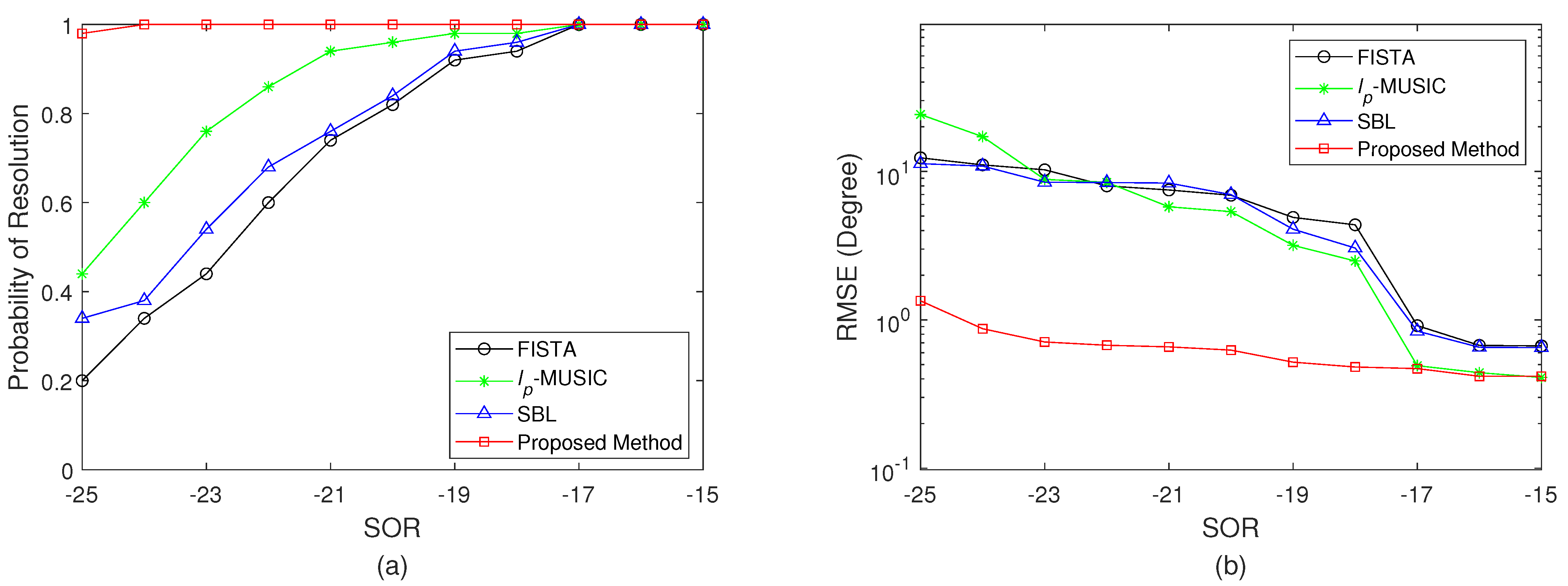
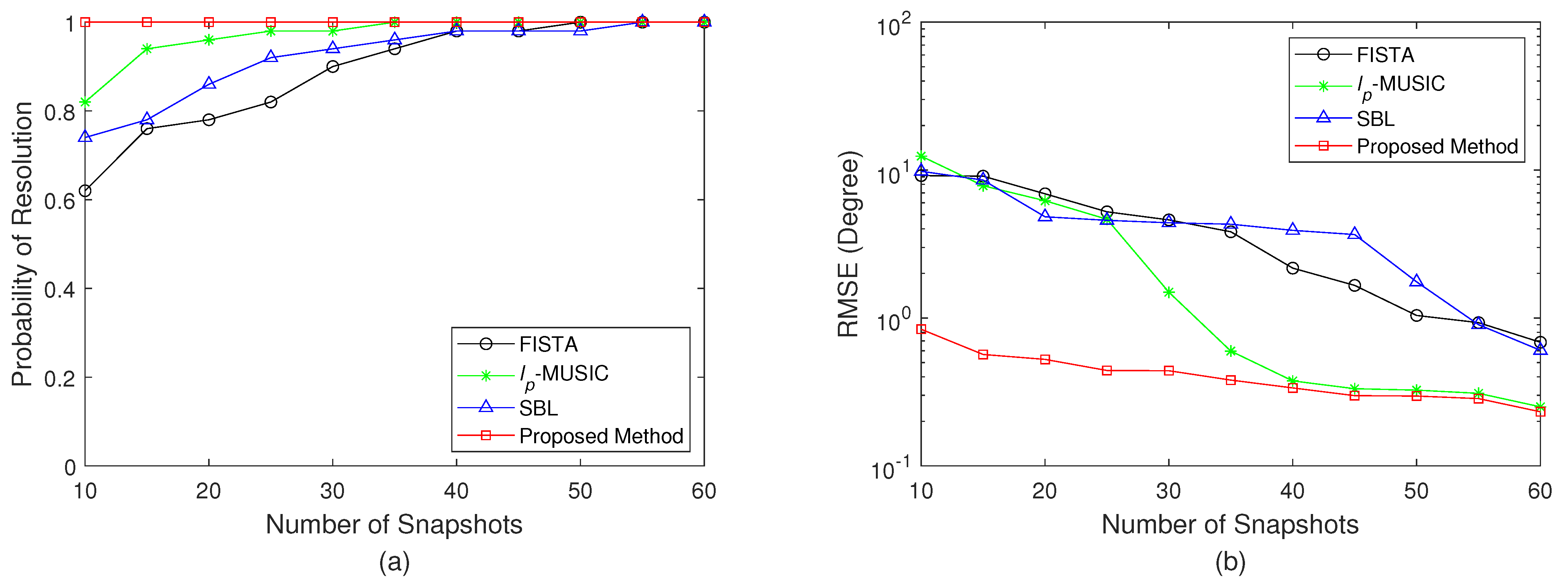
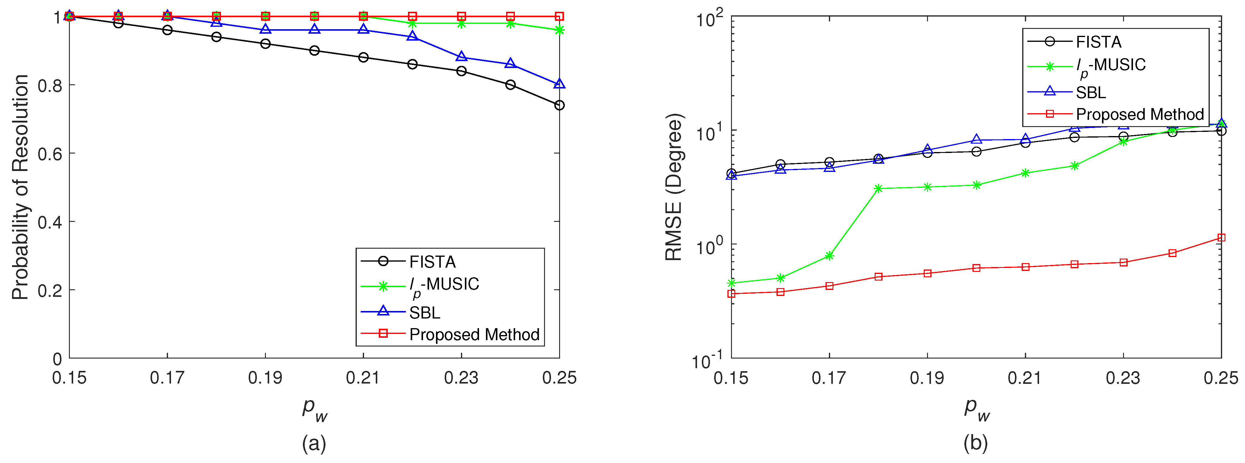
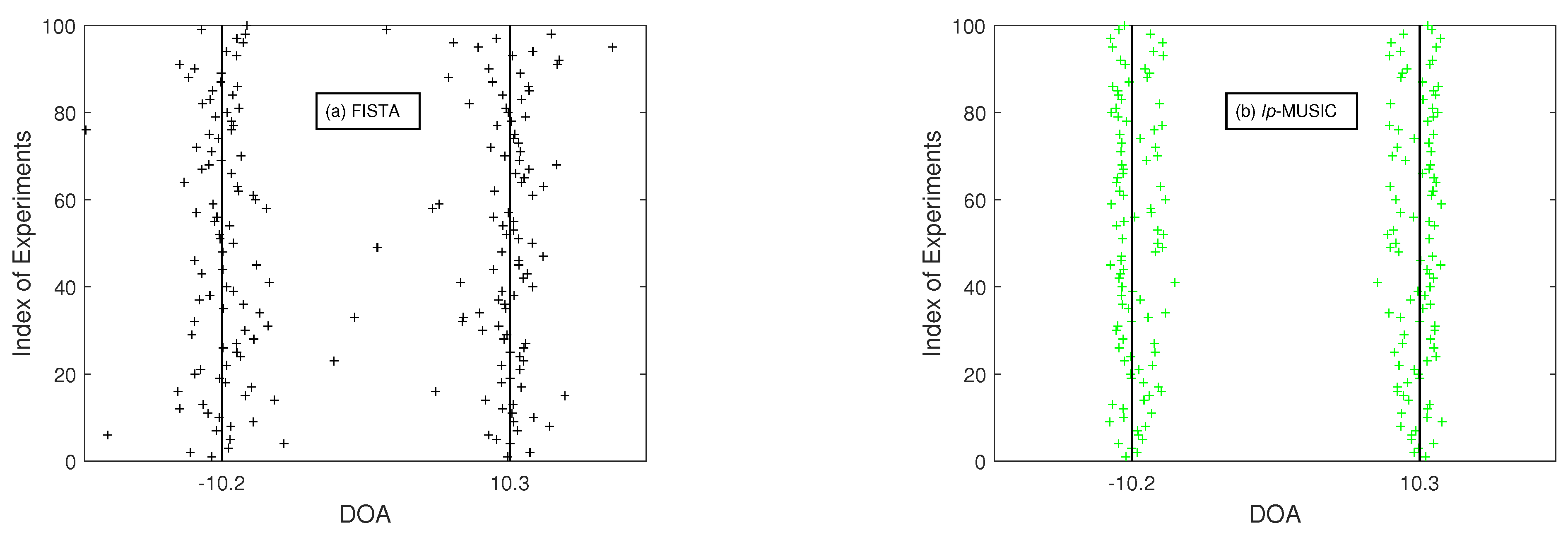
4. Simulation Results

In this section, we present simulations to assess the DOA estimation performance of the proposed method for impulsive noise. In the simulations, we assume two QPSK (quadrature phase shift keying) signals of the same power impinging on a ULA of sensors. The DOAs of the two incoming signals are ${\theta }_1=-10.2^{\circ }$ and ${\theta }_2=10.3^{\circ }$, respectively. The number of sensors is $M=12$. In each simulation, 100 Monte Carlo trials are run for each algorithm. The probability of resolution and the RMSE (root mean square error) are evaluated for each algorithm for comparison. Among them, a successful resolution is considered when the DOA estimation error for each source is less than $5^{\circ }$. The RMSE of the DOA estimates is calculated by

$$\mathrm{RMSE}=\sqrt{\frac{1}{KQ}\sum _{k=1}^K\sum _{q=1}^Q{({\widehat{\theta }}_{q,k}-{\theta }_q)}^2}$$

(22)

where K represents the number of the Monte Carlo runs, ${\theta }_q$ represents the real DOA of the q-th signal, and ${\widehat{\theta }}_{q,k}$ represents the estimate to ${\theta }_q$ in the k-th Monte Carlo run. The $l_p$-MUSIC, the FISTA-based method in [27], and the SBL-based method in [21] are performed for comparison. For $l_p$-MUSIC, as recommended in [8], $p=1.1$ is employed.

In the simulations, the variance of the Gaussian noise is assumed to be ${\sigma }_n^2$, and ${\left\{\mathbf{w}\left(t\right)\right\}}_{t=1}^T={\{\mathbf{b}\left(t\right)\odot {\mathbf{n}}_w\left(t\right)\}}_{t=1}^T$ is utilized to model the impulsive noise, where ${\left\{{\mathbf{b}}_i\left(t\right)\right\}}_{i=1}^M$ are Bernoulli distributed with $P({\mathbf{b}}_i\left(t\right)=1)=p_w$, that is, $p_w$ represents the probability of occurrence of the outliers, and ${\mathbf{n}}_w\left(t\right)$ is Gaussian distributed with zero-mean and variance ${\sigma }_w^2$. Accordingly, let ${\sigma }_s^2$ be the variance of signal, and the signal-to-noise ratio (SNR) is defined as $\mathrm{SNR}={\sigma }_s^2/{\sigma }_n^2$, whereas the signal-to-outlier ratio (SOR) is defined as $\mathrm{SOR}={\sigma }_s^2/{\sigma }_w^2$.

In the first experiment, the SNR is set at 20 dB, and $p_w$ is set at 0.2. The number of the data samples is $T=30$. Figure 1 shows the performance of the algorithms as a function of the SOR level. Obviously, as the SOR decreases, for each algorithm, the resolution probability deteriorates and the RMSE increases as expected. However, the RMSE of the proposed method demonstrates an improvement over the other three algorithms especially when the SOR is at extremely low levels. Another observation is that the resolution probability of the proposed method remains 1 for all the SOR values, whereas the other three algorithms present a distinct decrease, especially for low SOR values, indicating that our method obtains a more robust DOA estimation performance. Furthermore, this also explains why the RMSEs of the other three algorithms degrade so dramatically at extremely low SOR levels, as these methods yield DOA estimates with large deviations from the true DOAs in some of the trials.

In the following two experiments, the SNR and SOR of each algorithm are fixed at 20 dB and −20 dB, whereas $p_w$ is set at 0.15 for the former experiment and the number of snapshots for the latter experiment is $T=30$. Figure 2 and Figure 3 show the performance of the algorithms as a function of the number of the data samples and $p_w$, respectively. As Figure 2 and Figure 3 indicate, the proposed method presents a more robust performance over the other three methods when few snapshots are available or when $p_w$ increases, which indicates a higher occurrence probability of outliers.

In the last experiment, we assume that there are two coherent signals impinging on the array. The SNR and SOR are set at 20 dB and −20 dB, respectively. $p_w$ is set at 0.2. The number of snapshots is $T=30$. Figure 4 shows 100 realizations of the DOA estimates of these four algorithms. As shown in Figure 4, the DOA estimation results of the $l_p$-MUSIC [8], the FISTA-based method [27] and the SBL-based method [21] present a fairly large deviation with the real DOAs in the realizations, and the proposed method gains a much more accurate DOA estimation. This also proves that our proposed method is not only robust for uncorrelated signals but also for coherent signals.

5. Conclusions

In this paper, we present a new FISTA-based algorithm for DOA estimation in impulsive noise. By modelling the impulsive noise as the superposition of outliers in Gaussian noise, it is convenient to investigate the spot-sparse characteristic of the outlier matrix. For the array output, we implement FISTA via snapshot to obtain the estimates of the outlier matrix and the on-grid DOAs. Based on the estimated outlier matrix and the coarse on-grid DOA estimates, an alternate optimization method is developed to gain the final off-grid DOA estimates. Simulation results demonstrate that the proposed method presents more robust DOA estimation performance in extremely impulsive noise environments. In addition, the proposed method relaxed the uncorrelation assumption for the signals which is needed in the existing FISTA-based DOA estimation method, and its robust DOA estimation performance for coherent signals is demonstrated by simulations.

References

1. Johnson, D.H.; Dan, E.D. Array Signal Processing: Concepts and Techniques; Prentice-Hall: Englewood Cliffs, NJ, USA, 1993. [Google Scholar]
2. Krim, H.; Viberg, M. Two decades of array signal processing research: The parametric approach. IEEE Signal Process. Mag. 1996, 13, 67–94. [Google Scholar] [CrossRef]
3. Schmidt, R. Multiple emitter location and signal parameter estimation. IEEE Trans. Antennas Propag. 1986, 34, 276–280. [Google Scholar] [CrossRef] [Green Version]
4. Roy, R.; Kailath, T. ESPRIT-estimation of signal parameters via rotational invariance techniques. IEEE Trans. Acoust. Speech Signal Process. 1989, 37, 984–995. [Google Scholar] [CrossRef] [Green Version]
5. Rao, B.; Hari, K. Performance analysis of Root-Music. IEEE Trans. Acoust. Speech Signal Process. 1989, 37, 1939–1949. [Google Scholar] [CrossRef]
6. Nikias, C.L.; Shao, M. Signal Processing with α-Stable Distributions and Applications; John Wiley & Sons: New York, NY, USA, 1995. [Google Scholar]
7. Zhidkov, S.V. Analysis and comparison of several simple impulsive noise mitigation schemes for OFDM receivers. IEEE Trans. Commun. 2008, 56, 5–9. [Google Scholar] [CrossRef]
8. Zeng, W.J.; So, H.C.; Huang, L. p-MUSIC: Robust Direction-of-Arrival Estimator for Impulsive Noise Environments. IEEE Trans. Signal Process. 2013, 61, 4296–4308. [Google Scholar] [CrossRef]
9. Tsakalides, P.; Nikias, C. The robust covariation-based MUSIC (ROC-MUSIC) algorithm for bearing estimation in impulsive noise environments. IEEE Trans. Signal Process. 1996, 44, 1623–1633. [Google Scholar] [CrossRef]
10. Liu, T.H.; Mendel, J. A subspace-based direction finding algorithm using fractional lower order statistics. IEEE Trans. Signal Process. 2001, 49, 1605–1613. [Google Scholar] [CrossRef]
11. Swami, A.; Bm, S. On some detection and estimation problems in heavy-tailed noise. Signal Process. 2002, 82, 1829–1846. [Google Scholar] [CrossRef]
12. Huber, P.J. Robust Statistics; Springer: Berlin/Heidelberg, Germany, 2011. [Google Scholar]
13. Lee, D.D.; Kashyap, R.L. Robust maximum likelihood bearing estimation in contaminated Gaussian noise. IEEE Trans. Signal Process. 1992, 40, 1983–1986. [Google Scholar] [CrossRef]
14. Liao, B.; Zhang, Z.G.; Chan, S.C. A New Robust Kalman Filter-Based Subspace Tracking Algorithm in an Impulsive Noise Environment. IEEE Trans. Circuits Syst. II Express Briefs 2010, 57, 740–744. [Google Scholar] [CrossRef] [Green Version]
15. Chan, S.; Wen, Y.; Ho, K. A robust past algorithm for subspace tracking in impulsive noise. IEEE Trans. Signal Process. 2006, 54, 105–116. [Google Scholar] [CrossRef] [Green Version]
16. Visuri, S.; Oja, H.; Koivunen, V. Subspace-based direction-of-arrival estimation using nonparametric statistics. IEEE Trans. Signal Process. 2001, 49, 2060–2073. [Google Scholar] [CrossRef]
17. Malioutov, D.; Cetin, M.; Willsky, A. A sparse signal reconstruction perspective for source localization with sensor arrays. IEEE Trans. Signal Process. 2005, 53, 3010–3022. [Google Scholar] [CrossRef] [Green Version]
18. Hyder, M.M.; Mahata, K. Direction-of-Arrival Estimation Using a Mixed 2,0 Norm Approximation. IEEE Trans. Signal Process. 2010, 58, 4646–4655. [Google Scholar] [CrossRef]
19. Xu, X.; Wei, X.; Ye, Z. DOA Estimation Based on Sparse Signal Recovery Utilizing Weighted l1-Norm Penalty. IEEE Signal Process. Lett. 2012, 19, 155–158. [Google Scholar] [CrossRef]
20. Yin, J.; Chen, T. Direction-of-Arrival Estimation Using a Sparse Representation of Array Covariance Vectors. IEEE Trans. Signal Process. 2011, 59, 4489–4493. [Google Scholar] [CrossRef]
21. Dai, J.; So, H.C. Sparse Bayesian Learning Approach for Outlier-Resistant Direction-of-Arrival Estimation. IEEE Trans. Signal Process. 2018, 66, 744–756. [Google Scholar] [CrossRef]
22. Lee, G.C.F.; Rawat, A.S.; Wornell, G.W. Robust Direction of Arrival Estimation in the Presence of Array Faults using Snapshot Diversity. In Proceedings of the 2019 IEEE Global Conference on Signal and Information Processing (GlobalSIP), Ottawa, ON, Canada, 11–14 November 2019; pp. 1–5. [Google Scholar] [CrossRef]
23. Yang, Z.; Zhang, C.; Xie, L. Robustly Stable Signal Recovery in Compressed Sensing With Structured Matrix Perturbation. IEEE Trans. Signal Process. 2012, 60, 4658–4671. [Google Scholar] [CrossRef]
24. Huang, T.; Liu, Y.; Meng, H.; Wang, X. Adaptive matching pursuit with constrained total least squares. EURASIP J. Adv. Signal Process. 2012, 1, 1–12. [Google Scholar] [CrossRef] [Green Version]
25. Boyd, S.; Vandenberghe, L. Convex Optimization; Cambrige University Press: Cambrige, UK, 2004. [Google Scholar]
26. Beck, A.; Teboulle, M. A Fast Iterative Shrinkage-Thresholding Algorithm for Linear Inverse Problems. SIAM J. Imaging Sci. 2009, 2, 183–202. [Google Scholar] [CrossRef] [Green Version]
27. Tan, Z.; Yang, P.; Nehorai, A. Joint Sparse Recovery Method for Compressed Sensing with Structured Dictionary Mismatches. IEEE Trans. Signal Process. 2014, 62, 4997–5008. [Google Scholar] [CrossRef] [Green Version]
28. Carrillo, R.E.; Barner, K.E. Lorentzian Iterative Hard Thresholding: Robust Compressed Sensing with Prior Information. IEEE Trans. Signal Process. 2013, 61, 4822–4833. [Google Scholar] [CrossRef] [Green Version]
29. Yang, J.; Zhang, Y. Alternating Direction Algorithms for 1-Problems in Compressive Sensing. SIAM J. Sci. Comput. 2011, 33. [Google Scholar] [CrossRef]
30. Wen, F.; Liu, P.; Liu, Y.; Qiu, R.C.; Yu, W. Robust Sparse Recovery in Impulsive Noise via p-1 Optimization. IEEE Trans. Signal Process. 2017, 65, 105–118. [Google Scholar] [CrossRef]
Figure 1. Performance comparison of the algorithms as a function of the SOR. (a) Probability of resolution. (b) RMSE.
Remotesensing 15 00565 g001
Figure 2. Performance comparison of the algorithms as a function of the number of snapshots. (a) Probability of resolution. (b) RMSE.
Remotesensing 15 00565 g002
Figure 3. Performance comparison of the algorithms as a function of p w . (a) Probability of resolution. (b) RMSE.
Remotesensing 15 00565 g003
Figure 4. Performance comparison of the algorithms for coherent signals. (a) FISTA. (b) l p -MUSIC. (c) SBL. (d) Proposed method. The vertical lines denote the true DOAs, and the plus signs denote the DOA estimates in the experiments.
Remotesensing 15 00565 g004aRemotesensing 15 00565 g004b
Disclaimer/Publisher’s Note: The statements, opinions and data contained in all publications are solely those of the individual author(s) and contributor(s) and not of MDPI and/or the editor(s). MDPI and/or the editor(s) disclaim responsibility for any injury to people or property resulting from any ideas, methods, instructions or products referred to in the content.