Article

Unabated Global Ocean Warming Revealed by Ocean Heat Content from Remote Sensing Reconstruction

1
Key Laboratory of Spatial Data Mining and Information Sharing of Ministry of Education, The Academy of Digital China, Fuzhou University, Fuzhou 350108, China
2
Southern Marine Science and Engineering Guangdong Laboratory (Zhuhai), School of Marine Sciences, Sun Yat-sen University, Zhuhai 519000, China
3
Center for Remote Sensing, College of Earth, Ocean and Environment, University of Delaware, Newark, DE 19716, USA
4
Department of Geography, The University of Hong Kong, Hong Kong 999077, China
*
Author to whom correspondence should be addressed.
Remote Sens. 2023, 15(3), 566; https://doi.org/10.3390/rs15030566
Submission received: 7 December 2022 / Revised: 5 January 2023 / Accepted: 16 January 2023 / Published: 17 January 2023

Abstract

:
As the most relevant indicator of global warming, the ocean heat content (OHC) change is tightly linked to the Earth’s energy imbalance. Therefore, it is vital to study the OHC and heat absorption and redistribution. Here we analyzed the characteristics of global OHC variations based on a previously reconstructed OHC dataset (named OPEN) with four other gridded OHC datasets from 1993 to 2021. Different from the other four datasets, the OPEN dataset directly obtains OHC through remote sensing, which is reliable and superior in OHC reconstruction, further verified by the Clouds and the Earth’s Radiant Energy System (CERES) radiation flux data. We quantitatively analyzed the changes in the upper 2000 m OHC of the oceans over the past three decades from a multisource and multilayer perspective. Meanwhile, we calculated the global ocean heat uptake to quantify and track the global ocean warming rate and combined it with the Oceanic Niño Index to analyze the global evolution of OHC associated with El Niño–Southern Oscillation variability. The results show that different datasets reveal a continuously increasing and non-decaying global ocean warming from multiple perspectives, with more heat being absorbed by the subsurface and deeper ocean over the past 29 years. The global OHC heating trend from 1993 to 2021 is 7.48 ± 0.17, 7.89 ± 0.1, 10.11 ± 0.16, 7.78 ± 0.17, and 12.8 ± 0.26 × 10²² J/decade according to OPEN, IAP, EN4, Ishii, and ORAS5, respectively, which shows that the trends of the OPEN, IAP, and Ishii datasets are generally consistent, while those of EN4 and ORAS5 datasets are much higher. In addition, the ocean warming characteristics revealed by different datasets are somewhat different. The OPEN OHC dataset from remote sensing reconstruction shows a unique remote sensing mapping advantage, presenting a distinctive warming pattern in the East Indian Ocean. Meanwhile, the OPEN dataset had the largest statistically significant area, with 85.6% of the ocean covered by significant positive trends. The significant and continuous increase in global ocean warming over the past three decades, revealed from remote sensing reconstruction, can provide an important reference for projecting ocean warming in the context of global climate change toward the United Nations Sustainable Development Goals.

1. Introduction

In recent decades, greenhouse gas emissions from human activities (such as burning fossil fuels and deforestation) have contributed to the greenhouse effect, causing heat to be trapped in the Earth’s climate system and leading to global warming [1,2,3,4]. As a result, this leads to an imbalance of radiation at the top of the atmosphere (referred to as Earth’s Energy Imbalance, EEI) [5,6,7,8]. In addition, anthropogenic climate change has already affected every region, with an increase in the frequency and intensity of extreme heat, ocean heat waves, intense precipitation and ecological droughts, and reductions in Arctic sea ice, snowpack, and perennial permafrost [9,10,11]. The emissions of greenhouse gases, such as carbon dioxide and ozone, can lead to global climate change, and have played an important role in global heat absorption and redistribution [3,12,13]. Furthermore, the latest IPCC report states that global warming is accelerating and that global surface temperatures will continue to rise for at least this century [10].
At the same time, the ocean, as the vital regulator of the global climate system [14,15], covers a large area and holds nearly 97% of the worldwide water. Approximately 93% of the EEI is stored in the oceans [4,7,8]. Therefore, the heat change in the ocean system drives and reflects global climate change [16]. The majority of global warming heat eventually enters the ocean’s interior, is stored as thermal energy, and manifests as ocean warming [11,17]. However, the response of the oceans to increased atmospheric greenhouse gases has been slow and lagging, and impacts such as ocean warming from past carbon emissions will persist for several hundred years [10]. This phenomenon underscores the vital role of the oceans in global climate change. If humans achieve net-zero CO2 emissions soon, some of the impacts of climate change may be reversible. However, changes in the oceans, ice caps, and global sea levels will be irreversible for thousands of years [18].
As the most direct indicator for measuring ocean warming, ocean heat content (OHC) is a vital expression and directly reflects EEI [4,6,15]. Therefore, assessing global and regional OHC and its changing rate is crucial to monitoring the Earth’s climate change [14,19,20]. Since the change in EEI is very small, it is difficult to obtain it accurately. Therefore, some studies estimated the change in global OHC as an effective method to measure EEI [7,8]. Meanwhile, many studies have shown that the climate events in the oceans, such as the Interdecadal Pacific Oscillation (IPO) [21], the Atlantic Multidecadal Oscillation (AMO) [22], the Indian Ocean Dipole (IOD) [23,24], and El Niño–Southern Oscillation (ENSO) [25,26,27], are closely related to the OHC. As the most substantial time series disturbance of the climate system, ENSO is the primary mode of ocean-atmosphere interaction on interannual time scales in the climate system. Moreover, the manifestation of ENSO events in the oceans is closely related to the strong ocean heat distribution [25,28].
The latest IAP data show that the oceans are absorbing energy at an accelerating rate [11,29], with the upper 2000 m of the global ocean absorbing 14 × 1021 J more heat in 2021 than in 2020 [30]. For the past 80 years, the ocean has been warmer in each decade than in the previous one, with the deep ocean (700–2000 m) playing a critical role [15,31,32]. The increase of OHC in the 700–2000 m depth layer accounts for about 30% of the 0–2000 m increase in recent decades [33]. The new data suggest that warming in the North Pacific in 2021 extends from the surface to the deep ocean. At a depth of about 300 m, the oceans are warming by one degree Celsius [29]. However, horizontal and vertical ocean heat transfer affects heat uptake in the subsurface ocean, leading to a complex heat redistribution pattern [31,34]. During the global warming hiatus from 1998 to 2013, the increasing rate of global mean surface temperature (GMST) slowed down, while the opposite phenomenon occurs in the subsurface and deeper ocean. This hiatus is caused by heat sequestration and redistribution within the ocean. With the heat uptake and exchange at different layers in the ocean interior, more and more heat is stored in the subsurface and deeper ocean [35,36]. Meanwhile, to further understand the heat redistribution in different ocean basins during the hiatus period, several driving mechanisms have been proposed (such as natural variability, climate events, and the Indonesian throughflow (ITF)) [21,37]. Although slower than the upper layer, climate change in the subsurface and deeper layers of the ocean is an essential feature of anthropogenic global climate change [9,15]. Therefore, the deep ocean warming rate has become a fundamental feature of the Earth’s climate change [38]. This means that understanding how the ocean’s interior absorbs heat is crucial for future climate predictions [39]. However, several studies have estimated changes in historical OHC through climate simulations or data gap filling while suffering from significant uncertainties [9,40]. Previous studies on ocean warming mainly emphasized the application of in situ gridded and reanalysis data, lacking analysis from a remote sensing perspective. In recent years, many studies have reconstructed historical ocean interior information (such as OHC, subsurface temperature, and salinity, etc.) by combining satellite remote sensing data with artificial intelligence methods to reduce its uncertainty and achieve good performance [41,42,43,44,45].
This study revealed multilayered and multidimensional changes in global OHC in the upper 2000 m from 1993 to 2021. It also showed that the global ocean is continuously warming from multiple perspectives. The framework of this paper is as follows. Section 2 describes the data and methods used. Section 3 provides a comprehensive analysis of the global 0–2000 m OHC over the last three decades from several different perspectives, including time series variations and linear trends, revealing the global and regional evolution of the global OHC. Finally, Section 4 summarizes our results.

2. Materials and Methods

2.1. Materials

To analyze the multi-decadal variability and spatial and temporal patterns of global ocean heat content more directly, we used the OPEN OHC dataset from Fuzhou University. This data achieved temporal hindcast directly by artificial neural networks (ANN), machine learning methods based on remote sensing data (sea surface height, temperature, and wind), and spatiotemporal information (time, longitude, and latitude). Based on remote sensing data, the deep learning model can directly reflect the OHC information, reduce the uncertainty of the reconstructed OHC dataset, and improve the estimation accuracy. It provides a continuous record of the world’s OHC since 1993 at a resolution of 1° × 1° [41] (http://www.doi.org/10.11922/sciencedb.01058 (accessed on 1 April 2022)).
To comprehensively analyze global ocean warming in recent decades from multiple perspectives, we used various ocean subsurface temperature datasets as follows: (1) The Institute of Atmospheric Physics (IAP) of China, which provides a 3D gridded temperature dataset with Ensemble Optimal Interpolation (En-OI) mapping, combined with Coupled Model Intercomparison Project Phase 5 (CMIP5) multimodel datasets since 1940 at a resolution of 1° × 1° [31] (http://www.ocean.iap.ac.cn/ (accessed on 1 April 2021)). (2) EN4 (version 4.2.1 from the Hadley Met Office of the United Kingdom), a Gridded Spatial Objective Reanalysis Temperature-Salinity Dataset, used objective analysis (EN4-GR10, EN4-L09) to revise biases in existing observational datasets (e.g., WOD and Argo) since 1900 at a resolution of 1° × 1° [46] (https://www.metoffice.gov.uk/hadobs/en4/ (accessed on 1 April 2021)). (3) Ishii (from the Japan Meteorological Agency), a monthly mean dataset of global sea subsurface temperature and salinity. The period is from 1945 to 2021, the horizontal resolution is 1° × 1°, and it is vertically divided into 28 levels from 0 to 3000 m [47] (https://www.jma.go.jp/jma/en/menu.html (accessed on 1 April 2021)). (4) ORAS5 from the European Center for Medium-Range Weather Forecasts is a global ocean and sea ice reanalysis monthly dataset that assimilated various observational data in an ocean model since 1979 at a resolution of 1° × 1° [48] (https://www.cen.uni-hamburg.de/icdc/data/ocean/easy-init-ocean/ecmwf-oras5.html (accessed on 1 April 2021)).
To verify EEI estimated by OHC datasets, two types of EEI products are introduced: (1) the monthly top-of -atmosphere energy fluxes from the Clouds and the Earth’s Radiant Energy System (CERES) product [49] (https://ceres.larc.nasa.gov/data/ (accessed on 1 June 2022)), and (2) the MOHeaCAN v2.1 OHC-EEI product obtained using space altimetry and gravity measurements [8] (https://doi.org/10.24400/527896/a01-2020.003 (accessed on 1 June 2022)).
In addition, to capture the ocean surface information accurately, we used the SST dataset from NOAA’s Optimum Interpolation Sea Surface Temperature [50]. This dataset merged satellite and in situ data (i.e., ships and buoys) using the optimal interpolation method since 1981 at a resolution of 1° × 1° (https://psl.noaa.gov/data/gridded/data.noaa.oisst.v2.html (accessed on 1 April 2021)).
Moreover, we used an ENSO index to analyze the global ocean warming process related to ENSO variability on interannual scales. The Oceanic Niño Index (ONI), calculated from the HadISST1 [51], is the area-averaged SST between 5°S and 5°N and 170° and 120°W (the Niño 3.4 region). Before further analysis, the high frequency signals were filtered using a 12 month running mean to be consistent with the OHC signals (https://psl.noaa.gov/gcos_wgsp/Timeseries/Nino34/ (accessed on 1 April 2021)). Table 1 shows the information for all the data mentioned above.

2.2. Methods

OHC is calculated by integrating temperature within a layer. The calculation formula for the OHC (unit: J/m2) of each grid point is as follows:
    O H C = Z 0 C P ρ T d z
where Cp is the thermal capacity constant at 3850 J kg−1 °C−1; ρ is the constant density equal to 1025 kg m−3; T is the temperature; Z is the specified ocean depth.
This study divides the ocean into 27 layers from the surface to 2000 m. Here, OHC refers to the anomaly of OHC. The monthly climatology OHC data used in this study was constructed by a baseline period from 1993 to 2015. All OHC time series used a 12 month running mean to filter high frequency signals.
Moreover, linear regression coefficients calculated by the ordinary least squares method are used to quantify the long-term rate of global ocean warming. Meanwhile, we adopted a 95% confidence interval to determine the statistical significance of the heating trend uniformly.
To further analyze the change of ocean heat content over time, the global ocean heat uptake (OHU) is applied to quantify the heat uptake rate of the ocean. The OHU can be used to measure the importance of the ocean in climate warming. It has been proved that OHU is a good representative of EEI changes [8]. The OHU was calculated by the first-order time derivative of the global ocean heat content (GOHC), and the formula is as follows:
            O H U = d G O H C d t
Equation (2) can be discretized with a first-order centered difference based on the global OHC time series, if a fixed time step is adopted:
            y l ˙ = y l + 1 y l 1 2 Δ t ,   f o r   l     2 ,   n 1
where l is the time index; Δ t   is the length of one time step, which is one month here; y l is the OHC value at time l. For l = 1, we use a forward finite difference and for l = n, we use a backward finite difference scheme [8].
Before calculating OHU using the central difference method, the Lanczos filter is applied to a 1.5 to 8.5 year band-pass filter for the time series, to capture the interannual signals of OHU. The values of cut-off frequencies are based on previous studies [25,52].
Moreover, the EEI can be estimated by OHU obtained by the derivative of the GOHC dataset (Equation (4)), where α is 0.9, as estimated by von Schuckmann et al. [18].
  E E I = O H U α = 1 α d G O H C d t
Here, a linear regression model with the ONI as an independent variable was used to fit ocean heat anomalies associated with ENSO activity, which can be expressed as follows:
y = a · O N I + b + ε
where y is a time series of ocean heat variables; ONI is the Ocean Niño 3.4 Index; a is the slope; b and ε are intercept and error of this model, respectively. In this model, we perform lead and lag regression calculations by shifting the time series of y and ONI to analyze how the variable y changes with the phases of the ENSO event. When the time lag value is negative, it corresponds to the developing phases of the ENSO event; when the time lag value is 0, it corresponds to the peak phases of the ENSO event; when the time lag value is positive, it means the decaying phases of ENSO event.

3. Results

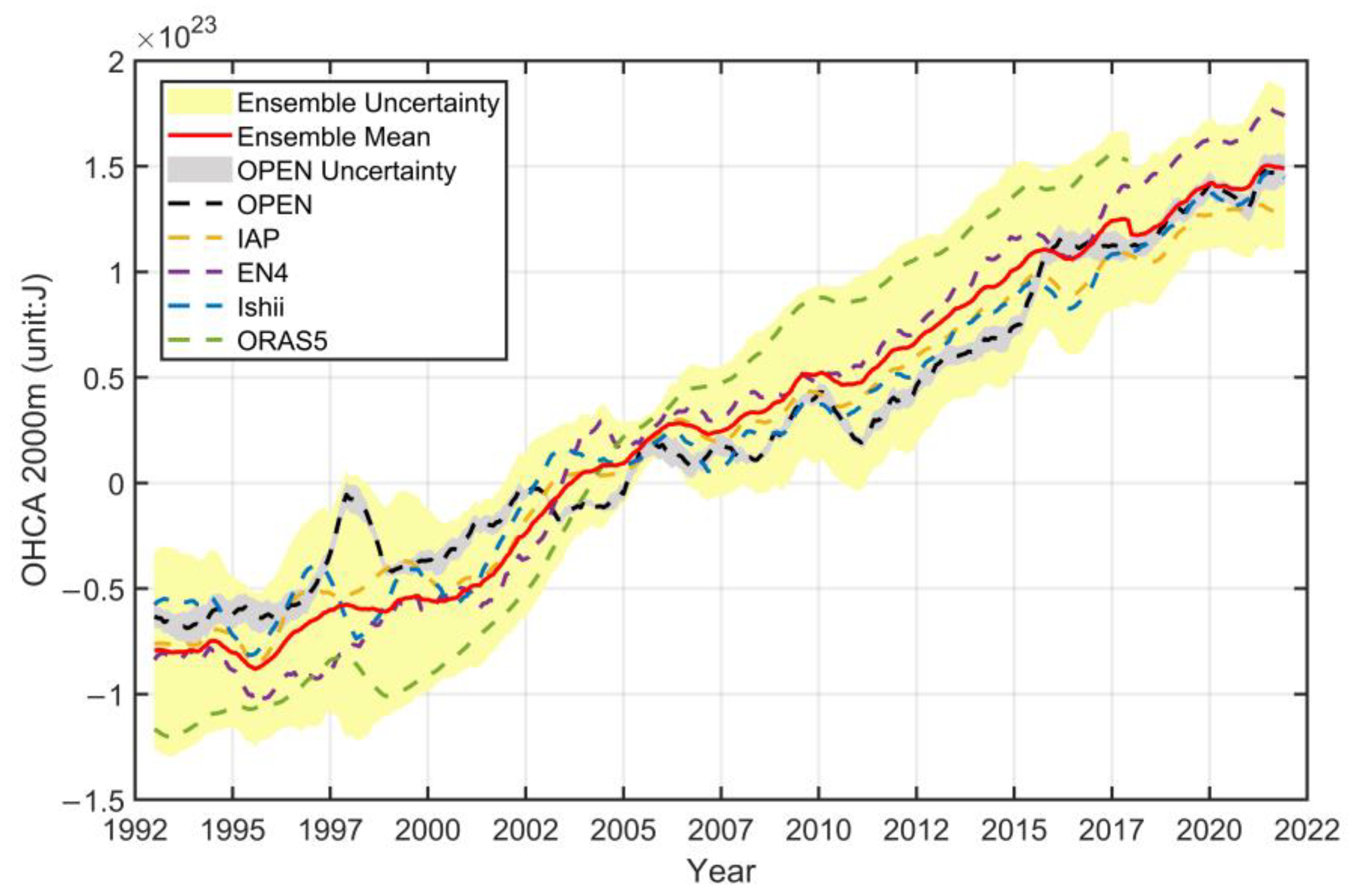
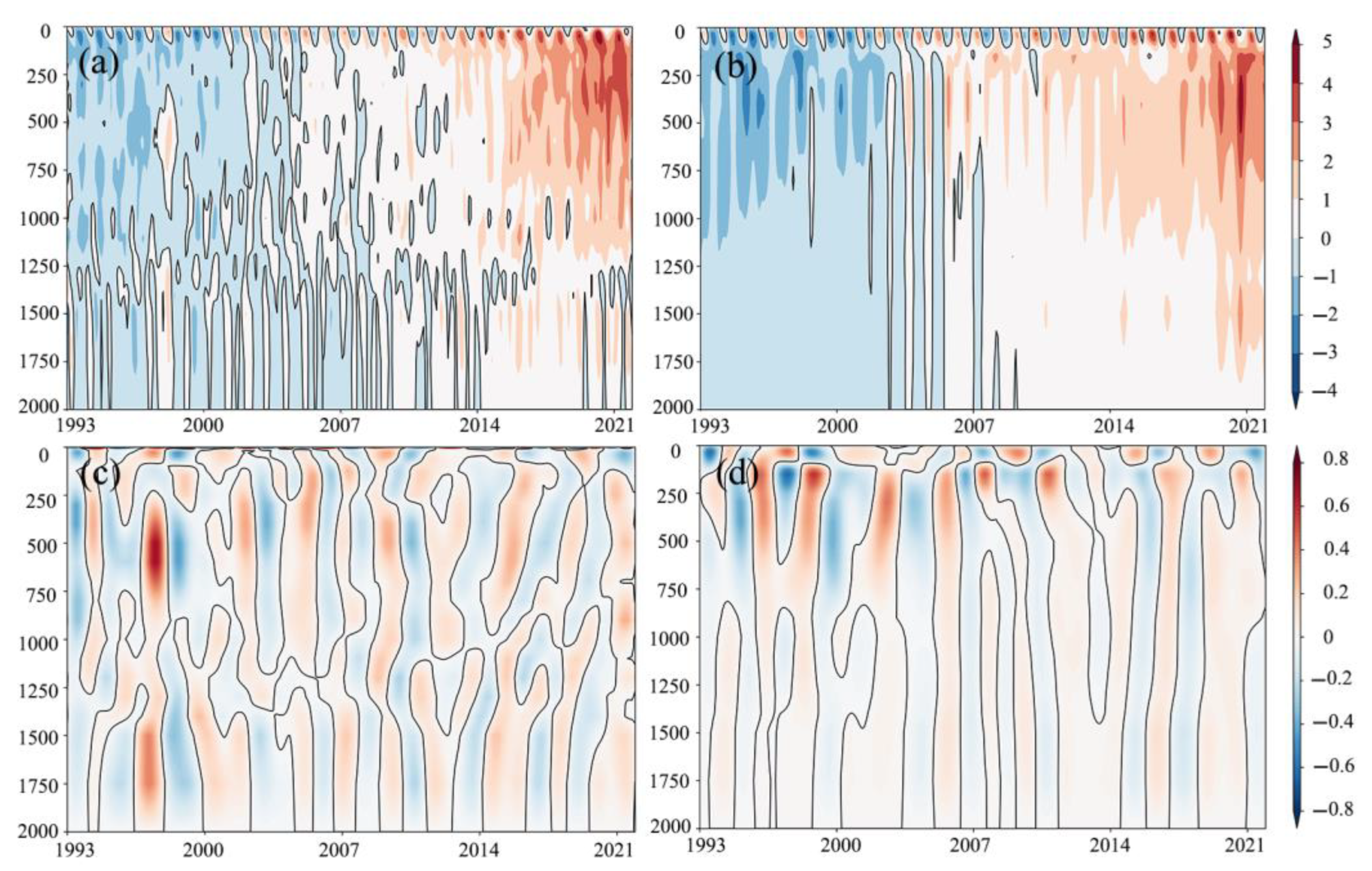
3.1. Time Evolution of OHC

Firstly, we used five datasets (OPEN, IAP, EN4, Ishii, and ORAS5) to analyze the temporal evolution of global ocean heat content from 0 to 2000 m (Figure 1). Figure 1 shows that the global ocean shows obvious interannual, decadal, and multidecadal changes from 0 to 2000 m. The global OHC trends from different datasets are generally consistent from 1993 to 2021. Overall, the OHC change from the five datasets shows an apparent upward trend on the decadal scale, indicating that the role of the worldwide ocean is becoming increasingly prominent in the context of global warming (Figure 1). These are consistent with the previous studies (e.g., [4,14,34]). Most of the heat from global warming ends up in the interior of the global ocean, and manifests itself as ocean warming.
However, the long-term heating trends of global OHC from 1993 to 2021 are somewhat different due to the different data sources and reconstruction methods for different datasets. For the OPEN dataset, the heating trend of global OHC from 1993 to 2021 is 7.48 × 10²² J/decade, while the heating trends based on IAP, EN4, Ishii, and ORAS5 are 7.89, 10.11, 7.78, and 12.8 × 10²² J/decade, respectively. Except for ORAS5, which covers the period from 1993 to 2017, the other four datasets all extend to 2021. Among them, the heating trend from the three datasets of OPEN, IAP, and Ishii are relatively close, while the EN4 and ORAS5 datasets are slightly higher (Figure 1). The latter four datasets were obtained by integrating the ocean 3D temperature dataset according to Equation 1, while the OPEN dataset obtains the global OHC directly through remote sensing reconstruction based on the machine learning method. Su et al. evaluated the accuracy of this dataset by the coefficient of determination (R2) and the relative root-mean-square error (RRMSE) and compared the results with the current mainstream OHC products. The R2 of the OPEN OHC dataset was greater than 0.95, and the RRMSE was less than 0.2, indicating a good overall effect [41].
The trends of the OPEN, IAP, EN4, Ishii, and ORAS5 datasets are relatively consistent (Figure 1). The ensemble mean is the average value of five datasets, which is close to the OPEN, EN4, IAP, and Ishii datasets as a whole, especially for the OPEN dataset. The statistical uncertainty of the OPEN dataset based on remote sensing reconstruction is represented by the gray shaded area in Figure 1. Specifically, for the OPEN dataset, by changing the training period (2005–2013, 2006–2014,…2010–2018) of the optimal artificial neural network, six training members are obtained, and the standard deviation of the six training members is taken as the statistical uncertainty [41]. The IAP, EN4, and Ishii datasets are all based on the original profile of WOD (World Ocean Datasets), and the datasets are reconstructed by selecting different XBT bias correction and mapping schemes [31,46,47]. Therefore, the statistical uncertainty of the three datasets mainly depends on the bias correction and gridded mapping method. Previous studies have analyzed the statistical uncertainty of the gridded datasets introduced by XBT bias correction and mapping schemes by the simple variable control method [40]. At the same time, the yellow shade in Figure 1 refers to the two times standard deviation of the five datasets. Among them, the ORAS5 from 1993 to 2005 is lower than the other four, while the overall ORAS5 from 2005 to 2021 is higher than the other datasets, and the slope of the ORAS5 dataset is slightly higher. After 2018, the statistical uncertainty calculated by the remaining four datasets decreased. The datasets after 2005 show more consistent trends, which is due to the unprecedented coverage and accuracy of the Argo network since 2005, in contrast to the XBT observation with more system bias and uncertainties.
To analyze the trends of OHC in different ocean basins, we take the OPEN dataset as an example, and divide the global ocean into four ocean basins (the Indian Ocean, the Atlantic Ocean, the Pacific Ocean, and the Southern Ocean). The interannual and decadal variations of OHC on global and basin scales in five depth ranges (0–100 m, 0–300 m, 0–700 m, 0–1500 m, and 0–2000 m) were well examined (Figure 2).
From 1993 to 2005, the global OHC is mainly concentrated in the upper layer, and the 0–100 m OHC anomaly is the highest (Figure 2a). However, since 2005, the global heat transferred from the upper layer to the subsurface and deeper layers, and the OHC anomaly gradually dispersed over time. Some studies have pointed out that intensified ocean heat vertical transport is the main reason for the “warming hiatus” phenomenon from 1998 to 2013 with Ishii and ORAS4 data [53]. Quantitatively, between 1999 and 2012, 1.22 × 1027 J of heat was trapped in the 300–1500 m layer of the oceans (Figure 2a). If this had not occurred, the upper 300 m of the ocean would have been as warm as the upper 1500 m since 1999. We calculated the OHC trends of the five datasets at different depth layers for consistency evaluation. Figure 2f shows that the ocean warming rate is gradually rising with the increase of integration depth, and the surface and deeper ocean warming are distinctive according to the different datasets. In the depth ranges of 0–700, 0–1500, and 0–2000 m, the OHC trends of the OPEN, IAP, and Ishii datasets are more consistent, while the trends of EN4 and ORAS5 are relatively higher.
To further examine the ocean warming status in different ocean layers and different periods, the average OHC trends and uncertainties are calculated based on the ensemble mean of the OPEN, IAP, EN4, and Ishii datasets (Table 2). We selected three periods: the whole period over the last three decades (1993–2021); since Argo data emerged until now (2005–2021); rapid ocean warming in the past decade (2011–2021). Table 2 shows that in each depth layer, global ocean warming accelerates distinctly over time. For example, within 0–2000 m, the warming rate increases from 0.88 W m−2 during 1993–2021 to 0.93 W m−2 during 2005–2021 and reaches as high as 1.11 W m−2 during 2011–2021.
All the datasets demonstrate that global OHC warming has accelerated at different depth layers over the past few decades. Furthermore, the heating trends in 0–300 m and 0–700 m of the upper ocean are more significant than that in 700–2000 m of the subsurface and deeper ocean. The heating trend of the 700–2000 m layer is relatively low, even slightly lower than the trend of the 0–300 m layer. Nevertheless, the rate of ocean warming at the subsurface and deeper layer still shows an increasing trend over time. Among all the periods, the uncertainty of the 0–2000 m layer over the 2011–2021 period reaches the maximum value of about 0.3 W m−2, which is mainly derived from the uncertainty at the 0–700 m layer. While the uncertainty of the 700–2000 m layer is only 0.08 W m−2 for the same period, indicating there is little difference in the warming rates of the subsurface and deeper ocean among the different datasets, and the distinctive warming in the subsurface and deeper layer is convincing.
Moreover, as shown in Figure 2, the heat uptake by the Atlantic and Pacific Oceans is more pronounced than the other ocean basins, which indicates that the Pacific and Atlantic Oceans dominate heat uptake in the global ocean. Several previous studies have analyzed the contribution of different ocean basins to global ocean heat absorption [35,36,40]. Therefore, we calculated the ratio of OHC of the four basins to the global ocean to quantitatively analyze their contributions to ocean heat uptake over the different periods. We divided the period from 1993 to 2021 (Figure 3a) into two periods: the pre-Argo era from 1993 to 2004 (Figure 3b) and the Argo era from 2005 to 2021 (Figure 3c). During the 1993–2021 period, all five datasets show the overall dominance of heat absorption in the Pacific and Atlantic oceans (Figure 3). During the period from 1993 to 2004, the five datasets show that the Atlantic Ocean and the Pacific Ocean dominated the global heat absorption, while the Southern Ocean showed a slightly negative contribution. Meanwhile, the contribution of the Indian and Southern Oceans to global heat absorption has increased in recent decades (Figure 3c). The contribution ratios obtained from different datasets are generally consistent, despite there being some discrepancies. Different from other datasets, the OPEN and ORAS5 datasets demonstrate that the Pacific Ocean and the Atlantic Ocean play dominant roles in the heat uptake of the global ocean during 1993–2021. Specifically, the heat absorption contribution of the Pacific Ocean is greater than that of the Atlantic Ocean, while other datasets show similar heat absorption contributions from the Pacific and Atlantic Oceans during 2005–2021.

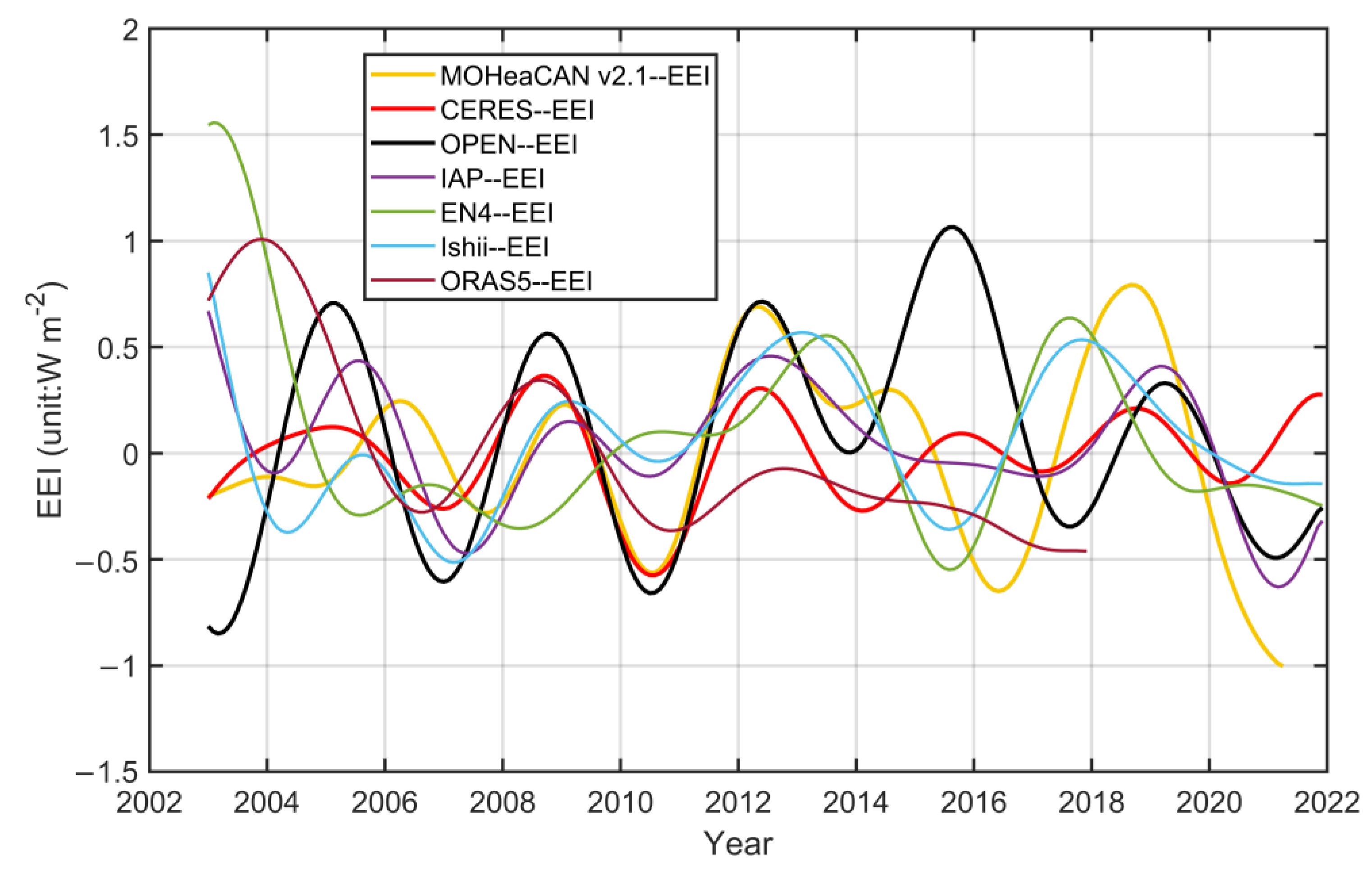
3.2. Earth’s Energy Imbalance for Validation

To directly compare the consistency and difference between different datasets at the interannual scale, two independent EEI estimates (MOHeaCAN and CERES) were applied to validate the OHC datasets. The MOHeaCAN dataset estimates global OHC changes based on spatial altimetry and gravity measurement, while CERES directly represents the incident and emitted radiation flux at the top of the atmosphere, which can directly estimate the EEI. When the net flux is positive the Earth is warming, while when it is negative the Earth is cooling. In addition, the EEI results obtained by other datasets used in this study (the OPEN, IAP, EN4, ORAS5, Ishii, and MOHeaCAN datasets) are indirectly estimated by OHC products. Therefore, the CERES dataset, as the measured data is directly obtained by satellite remote sensing, is the most reasonable choice to verify the reliability of the above datasets.
We removed trends and means from the EEI time series of each dataset, and then filtered out high frequency signals shorter than 3 years, which was speculated to be caused by errors in the measurement process instead of ocean warming [54]. As shown in Figure 4, in all EEI estimates, the OPEN dataset has a better correlation with CERES radiation flux compared with other datasets, although the amplitude is slightly higher in some years such as 2015/2016. From 2003 to 2021, most phases are consistent, especially from 2007 to 2014. Figure 4 shows that EEI estimated by the OPEN and MOHeaCAN datasets has a high consistency with CERES data during this period. In contrast, the EEI result estimated by the IAP dataset also has good performance, but the phase is inconsistent in some periods. The EEI time series estimated by the EN4 and Ishii datasets have a high correlation, but the overall phase is significantly different from the CERES results. The results of the ORAS5 dataset were better in the first few years but showed significant underestimation and insignificant amplitude in the later years. The main reason for the curve differences among the EEI estimates from different datasets is still unclear, and it has been suggested that they are influenced by climate variabilities in the ocean interior, such as ENSO (which may explain the higher amplitude of the EEI estimate by the OPEN dataset from 2015 to 2016). The other possible candidate could be the contribution of the ocean below 2000 m to heat storage, but some studies pointed out that the contribution is only about 0.07 W m−2 [8], which accounts for a minor portion of the EEI magnitude in Figure 4 at ~1 W m−2.

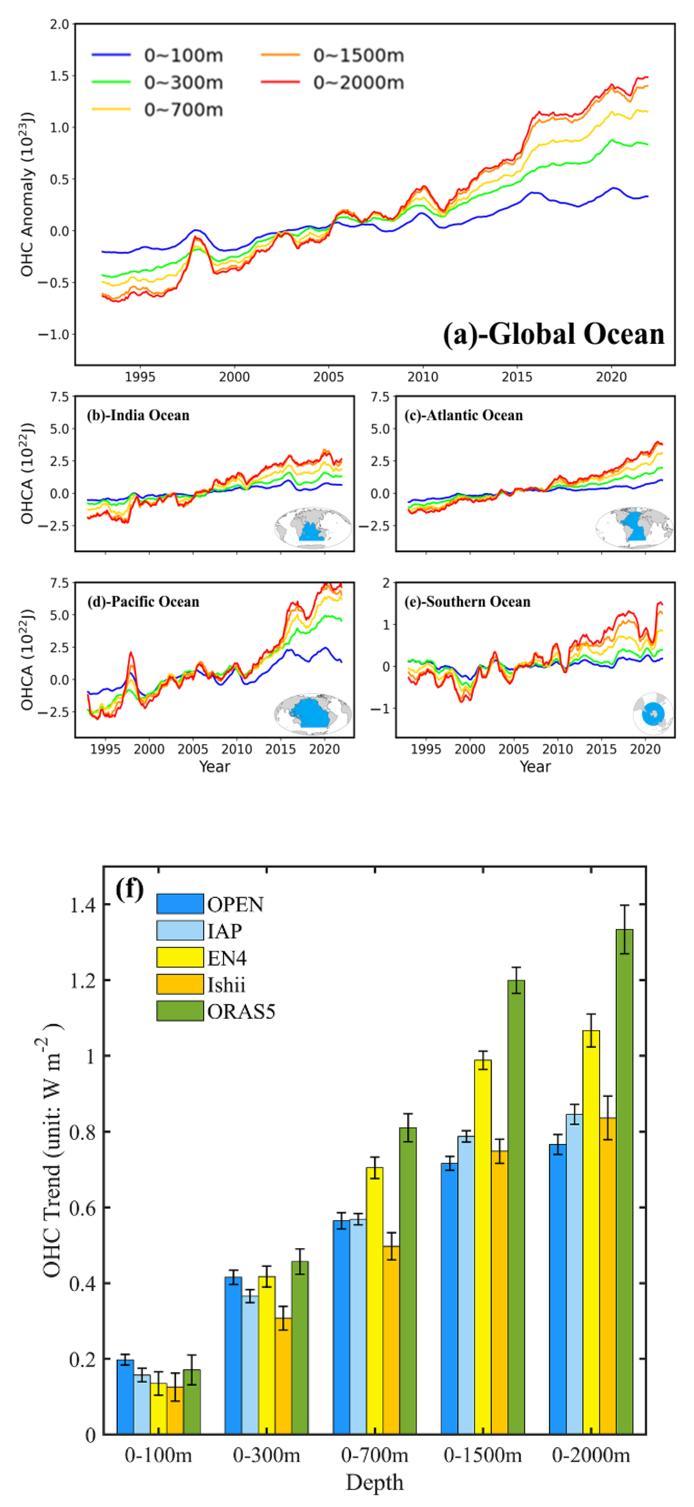
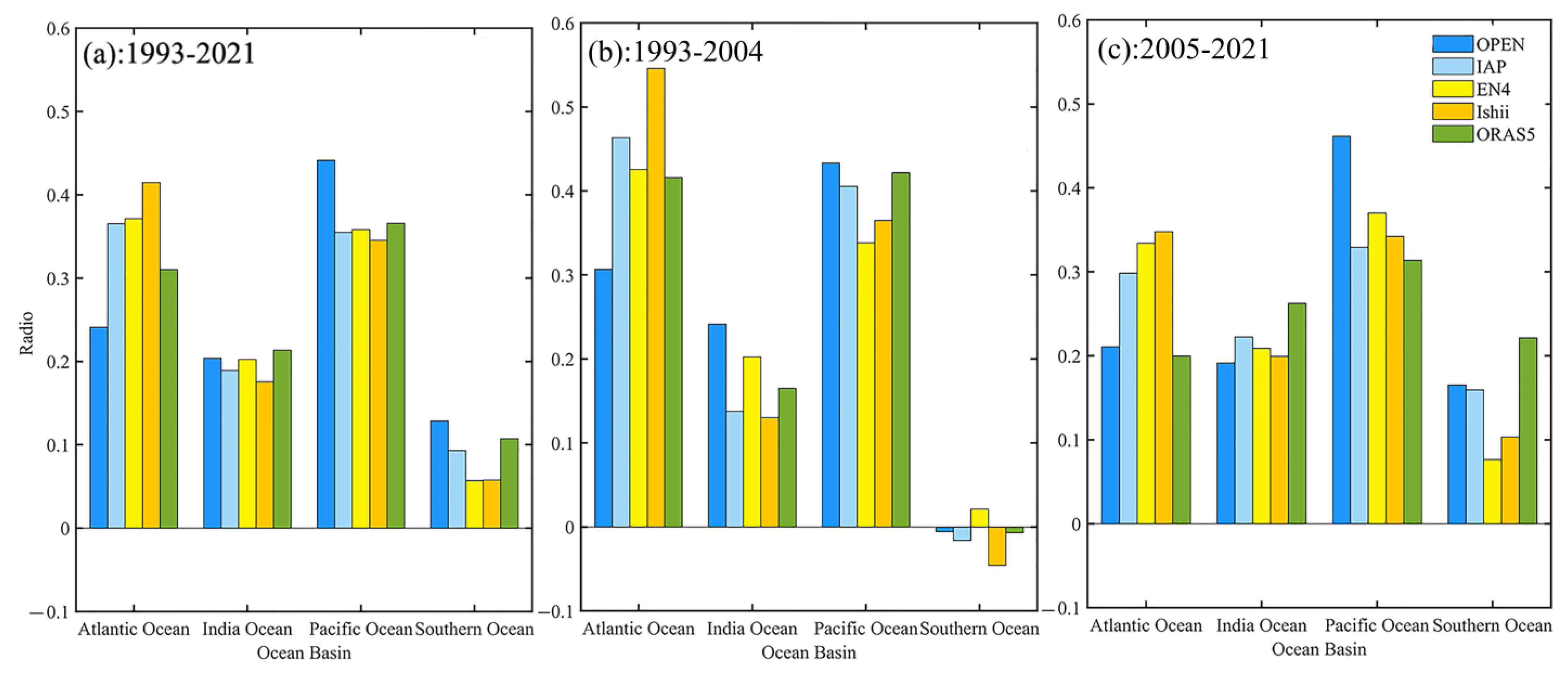
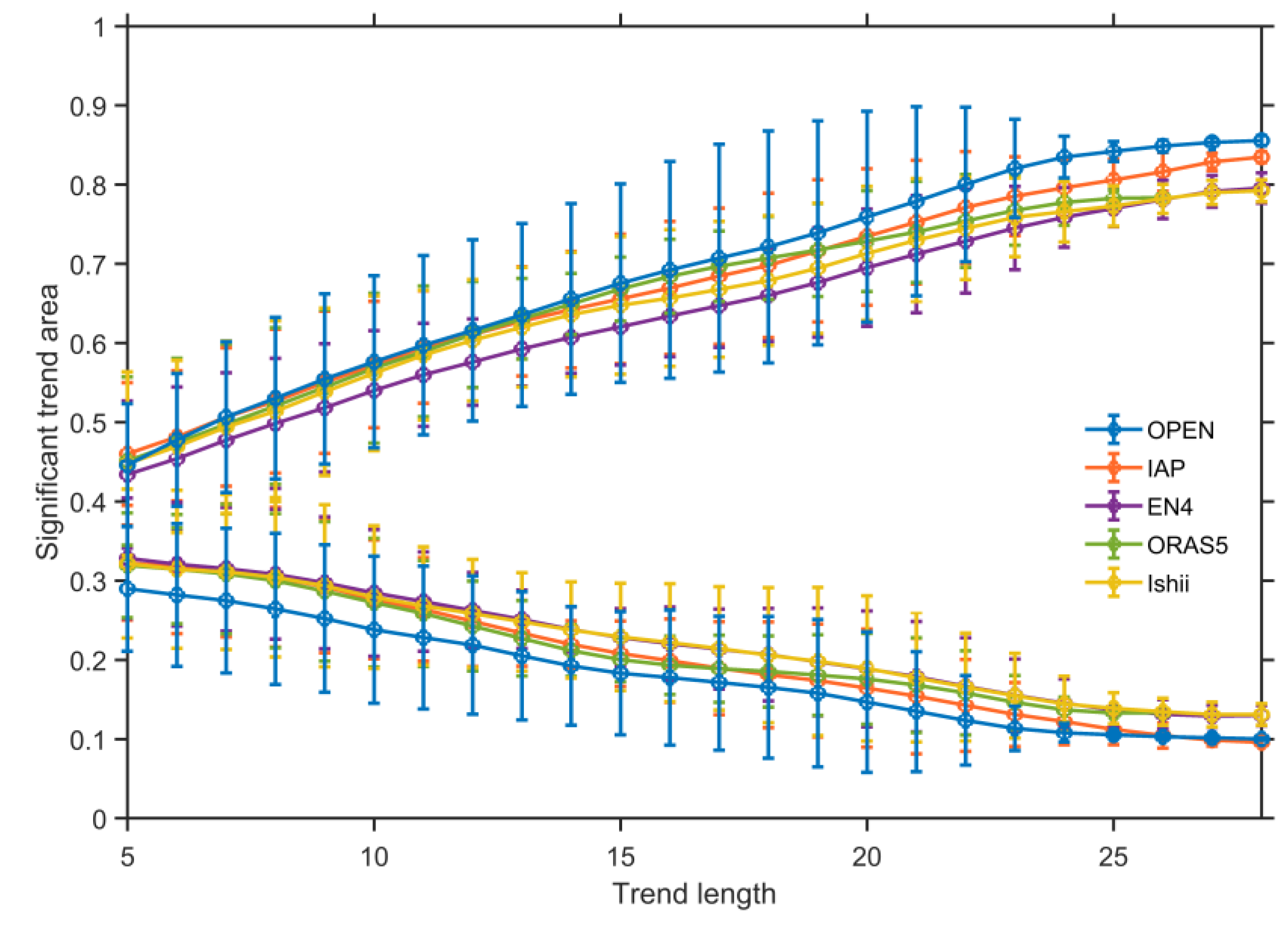
3.3. Global OHC Trends and Ocean Warming Tracking

To track global ocean warming and quantitatively analyze the heating trend of the global ocean in recent decades, we first adopted the least square method to linearly fit the OHC time series data to obtain its warming rate. As shown in Figure 5, during the global decadal warming process from 1993 to 2021, all ocean basins (including the Pacific, Atlantic, Indian, and Southern Oceans) showed significant warming. However, spatial heterogeneity of global ocean warming was observed. The warming characteristics of different ocean basins are different, and there are specific cooling phenomena in local ocean areas. On the other hand, a comparison of the spatial distribution maps of the heating trends of the five datasets confirms that the warming and cooling trends of the multiple datasets at 0–2000 m in the global ocean are relatively close (Figure 5).
As shown in Figure 5 and Table 3, the OPEN dataset shows 88.4% of the world’s global heating trend and 11.6% of the cooling trend from 1993 to 2021 (IAP: 87.5/12.5%, EN4: 83.6/16.4%, and ORAS5: 83.1/16.9%). In addition, we tested the significance of the linear trend of the OHC and found that the global warming range of the OPEN dataset narrowed to 85.6%, and the cooling rate narrowed to 10.0% (IAP: 82.9/9.7%, EN4: 79.1/13.4%, and ORAS5: 78.4/13.3%) from 1993 to 2021 (Table 3). Among them, the linear trend of the OPEN dataset had the largest area passing the significance test, followed by the IAP dataset. On the other hand, the OPEN dataset shows the strongest significant heating trend among the four datasets, followed by the IAP dataset. The relatively weakest significant heating trend was found in the ORAS5 dataset. Figure 5 shows the stippling area that failed the significance test of the IAP, EN4, and ORAS5 datasets are mainly concentrated at the regions with a trend close to 0, while the OPEN dataset has a smooth overall trend, and the regions that fail the significance test are small and scattered, which could show more details.
The zonal average of the global OHC linear trends is more correlated and shows consistency across the board (Figure 5e). The range of all four datasets is above 0, indicating a clear heating trend in the global ocean (biased toward warming, or the heating trend is much larger than the cooling trend). The OHC trends show a hemispheric asymmetry, and a noticeable bulge appears at 40°N and 40°S (Figure 5e). This is because the spatial warming distribution maps of the four datasets show a more pronounced heating trend near the mid-latitude Indian Ocean, the Pacific Ocean region, and the South Atlantic Ocean (Figure 5a–d). The IAP and EN4 datasets show the alternating phenomenon of warm and cold in the North Pacific Ocean, and many areas fail the significance test here, while the OPEN dataset shows a heating trend in this region, so the curve of Figure 5e is relatively flat with little fluctuation. In addition, the OPEN dataset shows a distinct cooling near 40°S (Figure 5a), while the IAP, EN4, and ORAS5 datasets show a general heating trend in the Southern Ocean with a stronger trend. This results in a flatter global OHC latitudinal mean result for the OPEN dataset near 40°S, with no apparent prominence (Figure 5e). This discrepancy may be related to the Antarctic Circumpolar Current near the Southern Ocean.
Figure 5f demonstrates the meridional mean trend of the global OHC. The range of the curve is greater than 0 in all five datasets, indicating that a meridional global heating trend is dominant. Meanwhile, the curve shows a bulge near 300°, which may be due to the large land area near 300° and the extreme warming process in the North Pacific Ocean, leading to a sudden increase near 300°. In addition, the OPEN dataset shows an evident warming phenomenon in the Indian Ocean that does not exist in other datasets, which may be related to the input variable—sea surface height (SSH) involved in remote sensing inversion. Therefore, the OPEN dataset result shows a prominent protrusion near 80°E (Figure 5f). This phenomenon is similar to the OHC trends calculated by Marti et al. using the MOHeaCAN dataset [8]. This may be the unique feature of the OPEN OHC from satellite remote sensing reconstruction, and the results may well reveal the warming phenomenon in the East Indian Ocean. Similarly, strong warming in the Southern Ocean and Indian Ocean from the ORAS5 dataset is represented as a distinct bulge in Figure 5f (green line).
To deeply analyze the change in the global ocean heating trend from 1993 to 2021, we selected 5–29 years as the step size of the global OHC linear trend (5 years: 1993–1997, 1994–1998, …, 2017–2021; 6 years: 1993–1998, 1994–1999,…, 2016–2021;…29 years: 1993–2021) [20], and took a class of each time step as an ensemble to calculate its ensemble mean value, and took the two times standard deviation of this ensemble as the uncertainty, which was represented as error bars in Figure 6. Based on the OPEN, IAP, EN4, ORAS5, and Ishii datasets, we selected 25 year steps ranging from 5 to 29 years as the steps to calculate the linear trend of OHC and calculated the regions with statistically significant positive and negative trends of global ocean warming from 1993 to 2021 (Figure 6).
As shown in Figure 6, with the increase of the step size, the statistically significant positive trend area in the global ocean increases, and the statistically significant negative trend area decreases with trend length, indicating that global ocean warming was unabated. This conclusion is consistent with the previous study by Johnson et al. [20]. Taking the OPEN dataset as an example, the average global warming area and global cooling area calculated based on the 5 year step linear fitting are 44.5% and 28.9%, respectively. Here, the area of the global OHC trend that passes the significance test is relatively small, as the degrees of freedom obtained by sliding over a 5 year time step are as low as 5.8. Therefore, as the time step increases, the global ocean area passing the significance test gradually increases. The error bars in Figure 6 are represented by 95% confidence intervals, i.e., two times standard deviation of the ensemble of linear trends with time steps ranging from 5 to 29 years of the OPEN dataset. When the time step is 15 to 20 years, the results are more uncertain. By comparing the global warming area ratio of the five datasets, the result of the OPEN dataset is very close to those of the other three datasets, except the EN4 dataset which shows a relatively small proportion of the global warming area. After the time step reaches 20 years, the result of the OPEN dataset is slightly larger than the other datasets. Until the time step reaches 25 years, the OPEN dataset result is closest to the result of the IAP dataset. At the same time, in the statistics of the proportion of global cooling area, the OPEN dataset shows a smaller global cooling area. As the time step increases, the difference among different datasets decreases, while the results of OPEN and IAP datasets are more similar, and the results of EN4 and Ishii datasets are closer.
Here, we further analyze the global ocean heat uptake using different datasets. The OPEN dataset combined with the well-used IAP dataset are used together to analyze and track the ocean heat uptake at different depth layers. As shown in Figure 7, the heat absorption efficiency of the ocean surface layer is small, but it fluctuates significantly during interannual climatic events such as ENSO (e.g., 1997/1998). The amplitude of the global OHU is the smallest at 700–2000 m depth layer, but the overall amplitude is greater than 0, indicating that the subsurface and deeper ocean are in a heating trend on the whole.
To more intuitively investigate the vertical distribution of global OHC over the past three decades, we plotted the depth-time map of OHC and OHU at a global scale (Figure 8). From 1993 to 2021, the OHC for both the OPEN and IAP datasets show an increasing trend over time in different ocean layers from a vertical profile perspective, and the heat significantly transfers from surface to subsurface and deeper layers (Figure 8a,b), verifying the conclusion in Figure 1 and Figure 2 that the oceans absorb most of the global warming heat and gradually transport deeper into the ocean. Interannual variations of global OHC can be observed in the upper 100 m ocean, with obvious alternation of cold and warm signals.
However, the main difference in global OHC vertical profiles between the two datasets is that the OPEN dataset shows more details of the warming signals in the subsurface ocean, while the IAP dataset is smoother and more consistent over the vertical profile. At the same time, a pronounced vertical OHC warming in the subsurface ocean was observed in the OPEN dataset with a large depth range around 1997–1998 (Figure 8a), which may be related to the strong El Niño phenomenon. In addition, OHU presents the alternations of cold and warm patterns over time in the ocean interior due to the influence of ENSO variability in different periods (Figure 8c,d). In particular, during the two intense El Niño events of 1997/1998 and 2015/2016, an apparent positive–negative alternation pattern occurred within the ocean. The OHU patterns in the upper 100 m ocean are somewhat opposite to those at the subsurface layer. The distinctive vertical heat redistribution and alternative patterns occurred in the ocean interior which may associate with ENSO variability.

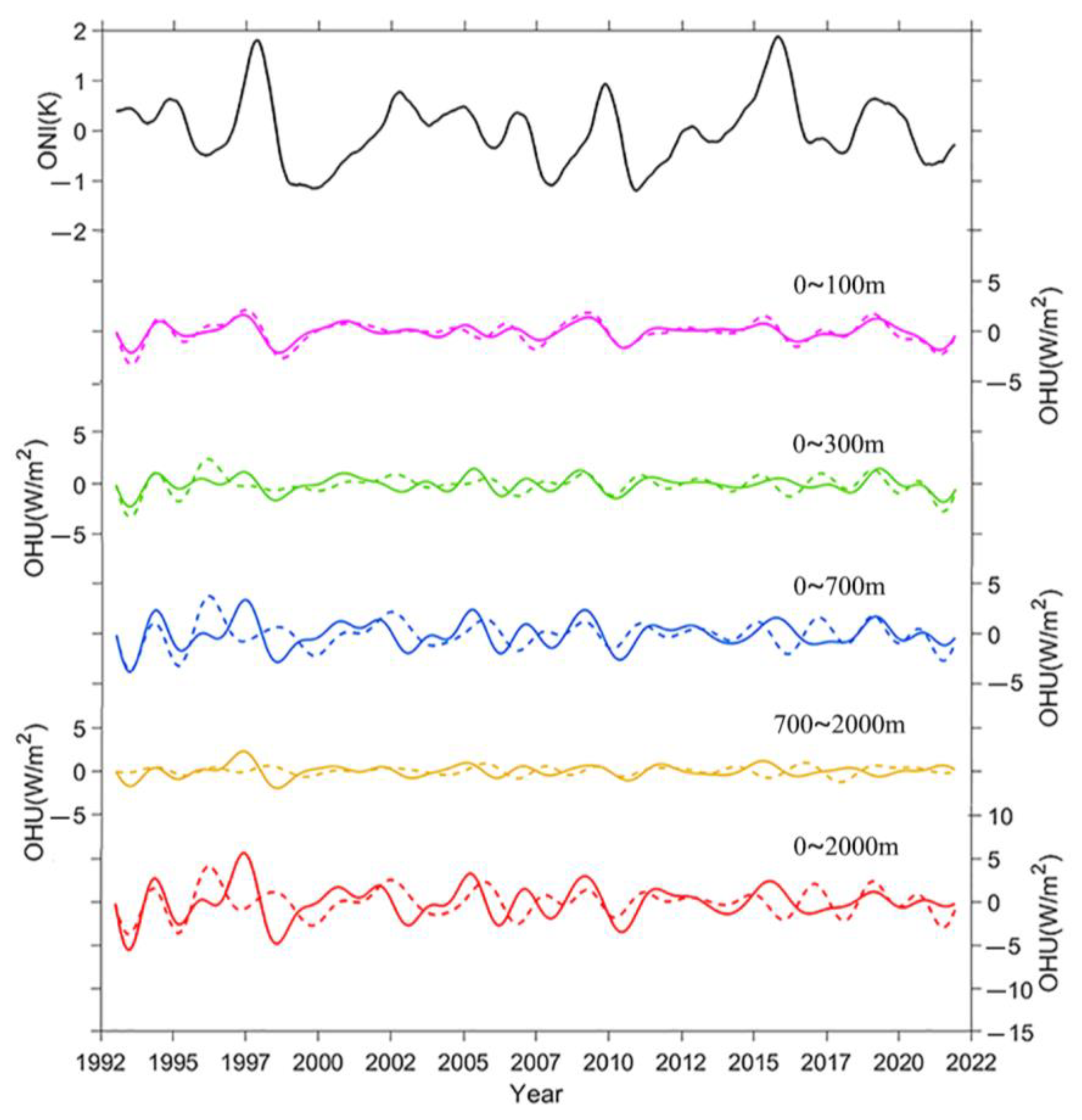
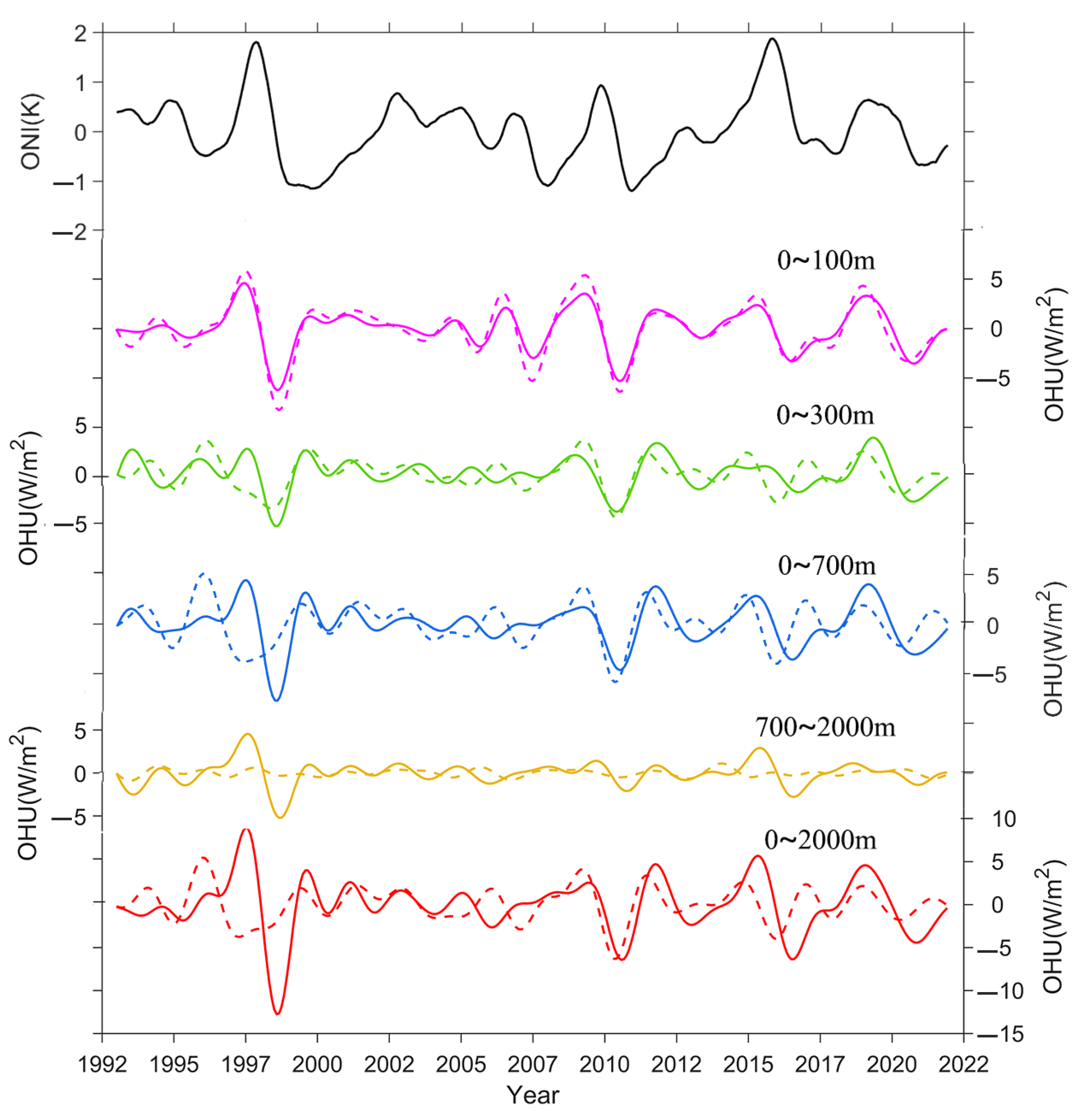
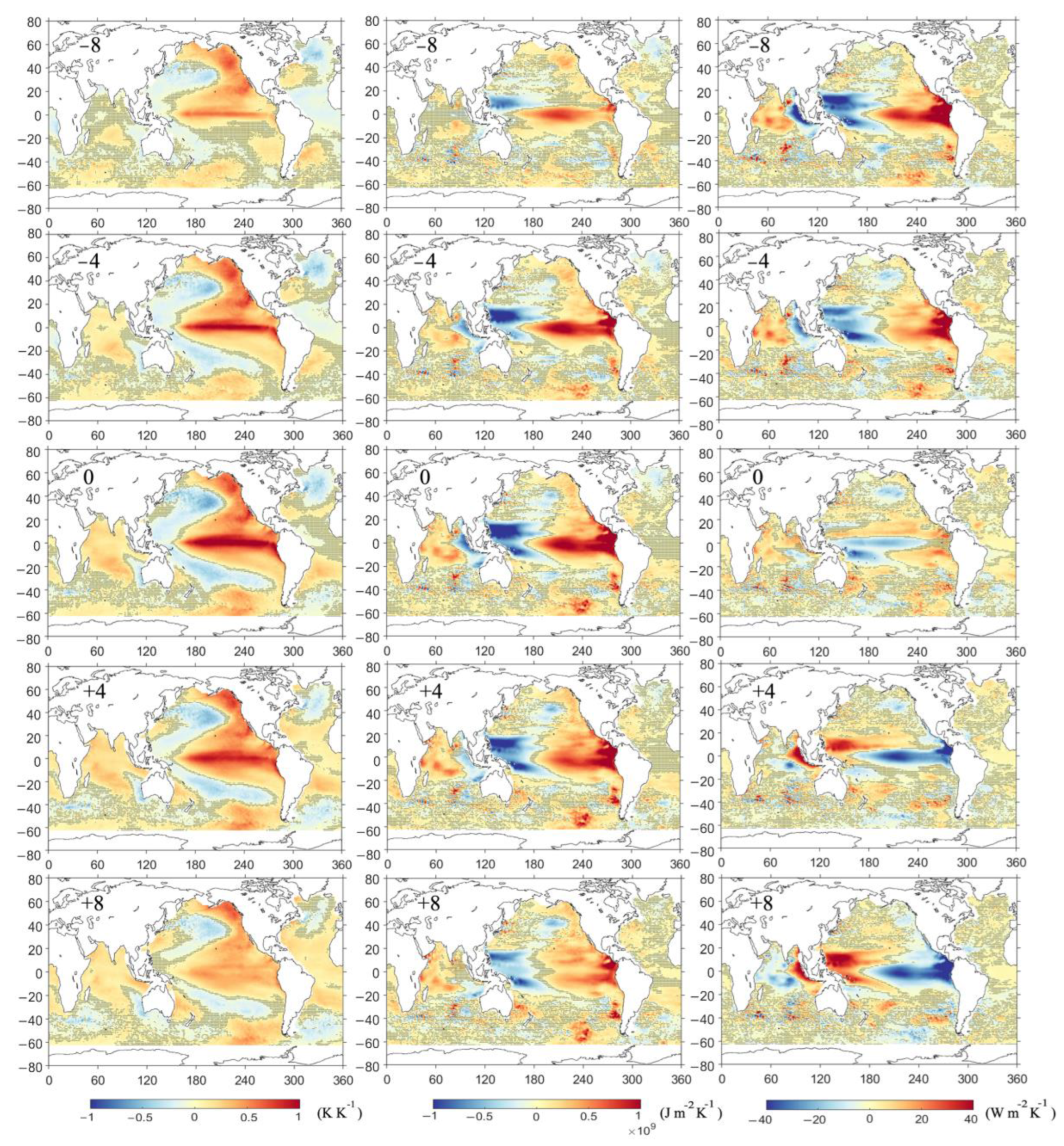
3.4. Global OHC Changes with ENSO

ENSO is the most active interannual oceanic climate factor. As shown in Figure 8c,d, ENSO variability has significant interannual disturbance to the changes of OHU in the ocean interior, leading to the interannual changes of global OHC. Furthermore, according to the OHU results, the global ocean presents a heating trend, and the OHU results of different depths show that the ENSO-related variability is the strongest signal of OHC variability on an interannual scale (Figure 7). Therefore, here we take the OPEN and IAP datasets as an example to explain the relationship between OHC and ENSO at different depth layers. To examine the relationship between OHU in the equatorial region and ENSO variability, we calculated OHU in the equatorial region (20°S~20°N) in addition to that in the global ocean (Figure 9).
The global ocean starts to lose heat at the onset of an El Niño event, and OHU also reaches a minimum after the peak of the El Niño event. Consistent with the previous studies (e.g., [25,26]), considering the two intense El Niño events in 1997/1998 and 2015/2016 as examples, the 0–100 m and 0–2000 m results in Figure 7 and Figure 9 show strong warming signals before the El Niño event. The OHU result also offers a more apparent downward trend after the El Niño event due to its energy release into the atmosphere. This may be related to the active vertical heat redistribution in the upper ocean during ENSO events. It’s worth noting that the OPEN dataset not only shows a strong ENSO signal in the 0–100 m upper ocean, but also shows an obvious bump of OHC anomaly in the subsurface and deeper ocean. Further investigation is needed to understand the mechanisms and causes of this phenomenon.
As shown in Figure 9, OHU variations for each depth layer in the equatorial region are more significant than those in Figure 7, indicating that OHU influenced by ENSO events is more intensive in the equatorial region. The OPEN and IAP datasets show good consistency, with the difference being that the IAP dataset is flatter in the 700–2000 m layer. The variability of OHU from 0 to 100 m in the equatorial region is highly correlated with the ONI variability, and the OHU variations of other depth layers are generally consistent with the ONI variation (Figure 9). Therefore, some scholars have pointed out that equatorial OHC is the primary source of ENSO predictability [25].
To analyze the pattern of global OHC variability before and after ENSO events, we calculated the lagged or leading correlation map of SST, OHC, and OHU onto ONI (Figure 10). In each case, linear regressions of the detrended anomalies of the above three variables were performed at each grid point of the ONI. Based on the linear regression of SST on the ONI, the spatial pattern shows the El Niño phenomenon (Figure 10, left column). The spatial distribution is characterized by warming in the central and eastern regions of the Pacific Ocean, extending north and south to the west coast of North and South America. In contrast, the western part of the Pacific Ocean shows a lateral U-shaped cooling phenomenon. This phenomenon is most apparent when the lag is zero (Figure 10, lag = 0). With the development of the El Niño event, the central Atlantic region evolved from cooling to warming.
However, the ocean OHC anomaly variability phenomenon for 0–2000 m during the ENSO event is more different from SST because the latter represents the sea surface information (Figure 10, middle column). In contrast, OHC is obtained by integrating subsurface and deeper temperatures inside the ocean with internal ocean signals. The spatial pattern changes in OHC anomalies mainly occur in the Pacific and Indian Oceans. With the development of the ENSO phenomenon (Figure 10, lag = −8, −4, 0, 4, and 8), the boundaries of cold and warm phenomena on the east and west sides of the central Pacific Ocean gradually shift westward during the zero-lag period, roughly on the exact boundary with SST at this moment. At the same time, the warming phenomenon in the eastern Pacific Ocean and the cooling phenomenon in the western Pacific Ocean show a strengthening and then weakening phenomenon. The contrast between the warming and cooling phenomena on the eastern and western sides of the Pacific Ocean is most evident during the zero-lag period, reaching a peak and extending to the southern and northern Pacific Ocean (Figure 10, middle column, lag = 0). During the ENSO phenomenon, the western Indian Ocean warms, and the eastern part cools with a clear reverse zonal gradient, which also peaks during the zero-lag period (Figure 10, middle column, lag = 0).
Meanwhile, OHU also shows more distinct variations during ENSO events, mainly distinguished in the Pacific and the Indian Ocean regions (Figure 10, right column). The eastern Pacific Ocean equatorial region shows a positive OHC increasing trend before the El Niño event (Figure 10, right column, lag = −8 and −4). The positive trend slowly decreases with the El Niño event to near zero during the zero-lag period. At this moment, a negative OHU phenomenon occurs in the western Pacific Ocean (Figure 10, right column), leading to an anomalous cooling of the OHC (Figure 10, middle column). In the Indian Ocean, on the other hand, El Niño is preceded by a dipole phenomenon, an anomalous climate oscillation in which the western side of the Indian Ocean continuously warms, and the eastern side reverses. The OHC in the equatorial Pacific and Indian Oceans peaks at the El Niño event, i.e., the zero-lag figure (Figure 10, middle column, lag = 0). At the same time, after the El Niño event, the equatorial eastern Pacific Ocean shows an opposite trend from the pre-event, i.e., negative growth. This trend keeps strengthening (Figure 10, right column, lag = 4 and 8), resulting in the OHC declining at this time. The IOD phenomenon also changes in the opposite direction, with the eastern side becoming warmer and the western side becoming more fabulous, and the contrast gradually intensifies. In conclusion, the dipole structures in the Pacific and Indian Oceans change in opposite directions with the development of El Niño events.

4. Conclusions

Using ocean remote sensing heat content dataset, combined with in situ observation datasets, and reanalysis datasets (OPEN, IAP, EN4, Ishii, and ORAS5), we demonstrated that the rate of ocean warming has not decreased but continued to increase, have quantified the global ocean warming rate over the past three decades, and analyzed how much ocean warming has occurred. The results show that between 1993 and 2021, heat in the oceans, the largest heat reservoir on Earth, also shows a trend of continuous increase against the backdrop of global warming. In addition, ocean heat uptake was mainly concentrated on the upper layer before 2005. Heat has gradually transferred to the subsurface and deeper ocean since 2005. The different ocean basins and different ocean depths present varying degrees of warming status.
The comparison between various datasets shows some differences among them. For example, the OPEN dataset, which is based on the direct estimation of OHC by satellite remote sensing, has better spatial and temporal consistency, and its spatial warming pattern is slightly different from that of the other four gridded datasets, especially in the East Indian Ocean. Nevertheless, the OHC changes from different datasets can indeed reveal the consistencies and discrepancies of warming status and patterns in the different layers of the ocean, enriching the perspectives of OHC evolution analysis. Meanwhile, we can recognize the remaining uncertainties of the global OHC change analysis. The inconsistencies between the different datasets may be due to discrepancies between the original input data and data mapping methods, as well as insufficient data in the deeper ocean. Among the five datasets, the results of the OPEN, IAP, and Ishii datasets are close to each other on the whole, while the EN4 and ORAS5 datasets show a slightly higher warming trend. Meanwhile, we adopted CERES radiation flux data to validate and confirm the reliability and advantage of the OPEN dataset. As a result, it accurately reveals the three-dimensional warming characteristics of the ocean has better performance in specific ocean climate events, and better reflects the pattern and details of heat changes within the global ocean. However, more important than variability among the five datasets, the results from various data sources reflect the consistency of global ocean warming. Over the past three decades, the global ocean has shown a consistently increasing and unabated warming rate. For the OPEN dataset, as the time step for global OHC trends increases from 5 to 29 years, the proportion of area with significant global heating trends greater than 0 expands from 44.5% to 85.6%, and the area with significant cooling shrinks from 28.9% to 10.0%. The other four datasets also show similar results, which confirms the progressive expansion of global ocean warming since 1993, proving the unequivocal, unprecedented, and irreversible characteristics of global warming.
In addition, considering the OPEN and IAP dataset as examples, we quantified global OHU with the central difference method to analyze global ocean warming rate changes over time in the recent 29 years. The results also confirmed that the global ocean is progressively warming. Through the quantification and analysis of ocean heat uptake, the change of heat in the ocean interior from 0 to 2000 m was tracked. Furthermore, the ENSO variability modulates the interannual and interdecadal variations of global ocean OHC and OHU. The OHC varies actively in the equatorial Pacific and Indian Ocean regions during the development and peak periods of El Niño events. As a result, there is a significant heat redistribution within the ocean, while the OHC shows a transient decrease during the El Niño decline.
Overall, the oceans have been warming unabatedly over the past few decades, and this trend will probably continue to increase rather than decrease in the future due to continuous global warming. Therefore, it is essential to effectively construct and predict the ocean heat content change and future ocean warming for coping with the global climate change issue. Meanwhile, under the background of global warming and carbon neutrality, it is necessary to accurately quantify and project the future warming rate of the ocean, which will provide more reliable scientific support for global climate change action and carbon neutrality implementation during recent global warming. By comparing the datasets from multiple perspectives, we find that the satellite-based deep ocean remote sensing technique provides a useful way for ocean heat content estimation and projection, which enables us to study global ocean warming and climate change from a remote sensing perspective. Future study also needs to further analyze the estimation errors and uncertainties and make further improvements in OHC remote sensing reconstruction, such as selecting more valuable input variables, and adopting more advanced deep learning methods with higher performance to produce datasets with higher resolutions and quality to support the global climate change and ocean warming studies.

Author Contributions

Conceptualization, H.S.; methodology, Y.W.; validation, Y.W.; formal analysis, H.S. and Y.W.; investigation, H.S. and Y.W.; data curation, Y.W.; writing—original draft preparation, H.S. and Y.W.; writing—review and editing, H.S., W.L. and H.Z.; visualization, Y.W.; supervision, H.S., W.L., H.Z. and X.-H.Y.; funding acquisition, H.S. and X.-H.Y. All authors have read and agreed to the published version of the manuscript.

Funding

This research was funded by the National Natural Science Foundation of China (41971384), the Natural Science Foundation for Distinguished Young Scholars of Fujian Province of China (2021J06014), the National Key R&D Program of China (2019YFA0606702) and the National Natural Science Foundation of China (91858202).

Data Availability Statement

The data presented in this study are available on request from the corresponding author.

Conflicts of Interest

The authors declare no conflict of interest.

References

  1. Cheng, L.; Trenberth, K.; Fasullo, J.; Boyer, T.; Schuckmann, K.; Zhu, J. Taking the Pulse of the Planet. Eos Trans. Am. Geophys. Union 2017, 98. [Google Scholar] [CrossRef]
  2. Tokarska, K.B.; Hegerl, G.C.; Schurer, A.P.; Ribes, A.; Fasullo, J.T. Quantifying human contributions to past and future ocean warming and thermosteric sea level rise. Environ. Res. Lett. 2019, 14, 074020. [Google Scholar] [CrossRef]
  3. Charles, E.; Meyssignac, B.; Ribes, A. Observational constraint on greenhouse gas and aerosol contributions to global ocean heat content changes. J. Clim. 2020, 33, 10579–10591. [Google Scholar] [CrossRef] [Green Version]
  4. Storto, A.; Balmaseda, M.A.; De Boisseson, E.; Giese, B.S.; Masina, S.; Yang, C. The 20th century global warming signature on the ocean at global and basin scales as depicted from historical reanalyses. Int. J. Climatol. 2021, 41, 5977–5997. [Google Scholar] [CrossRef]
  5. Trenberth, K.E.; Fasullo, J.T.; Balmaseda, M.A. Earth’s energy imbalance. J. Clim. 2014, 27, 3129–3144. [Google Scholar] [CrossRef] [Green Version]
  6. Trenberth, K.E.; Fasullo, J.T.; von Schuckmann, K.; Cheng, L. Insights into Earth’s Energy Imbalance from Multiple Sources . J. Clim. 2016, 29, 7495–7505. [Google Scholar] [CrossRef] [Green Version]
  7. Meyssignac, B.; Boyer, T.; Zhao, Z.; Hakuba, M.Z.; Landerer, F.W.; Stammer, D.; Köhl, A.; Kato, S.; L’Ecuyer, T.; Ablain, M.; et al. Measuring Global Ocean Heat Content to Estimate the Earth Energy Imbalance. Front. Mar. Sci. 2019, 6, 432. [Google Scholar] [CrossRef] [Green Version]
  8. Marti, F.; Blazquez, A.; Meyssignac, B.; Ablain, M.; Barnoud, A.; Fraudeau, R.; Jugier, R.; Chenal, J.; Larnicol, G.; Pfeffer, J.; et al. Monitoring the ocean heat content change and the Earth energy imbalance from space altimetry and space gravimetry. Earth Syst. Sci. Data 2022, 14, 229–249. [Google Scholar] [CrossRef]
  9. Cheng, L.; Abraham, J.; Hausfather, Z.; Trenberth, K.E. How fast are the oceans warming? Science 2019, 363, 128–129. [Google Scholar] [CrossRef] [PubMed]
  10. Arias, P.; Bellouin, N.; Coppola, E.; Jones, R.; Krinner, G.; Marotzke, J.; Naik, V.; Palmer, M.; Plattner, G.-K.; Rogelj, J. Climate Change 2021: The Physical Science Basis. Contribution of Working Group14 I to the Sixth Assessment Report of the Intergovernmental Panel on Climate Change. Tech. Summ. 2021. [Google Scholar] [CrossRef]
  11. Cheng, L.; Abraham, J.; Trenberth, K.E.; Fasullo, J.; Boyer, T.; Locarnini, R.; Zhang, B.; Yu, F.; Wan, L.; Chen, X.; et al. Upper Ocean Temperatures Hit Record High in 2020. Adv. Atmos. Sci. 2021, 38, 523–530. [Google Scholar] [CrossRef]
  12. Li, S.; Liu, W.; Lyu, K.; Zhang, X. The effects of historical ozone changes on Southern Ocean heat uptake and storage. Clim. Dyn. 2021, 57, 2269–2285. [Google Scholar] [CrossRef]
  13. Liu, W.; Hegglin, M.I.; Checa-Garcia, R.; Li, S.; Gillett, N.P.; Lyu, K.; Zhang, X.; Swart, N.C. Stratospheric ozone depletion and tropospheric ozone increases drive Southern Ocean interior warming. Nat. Clim. Change 2022, 12, 365–372. [Google Scholar] [CrossRef]
  14. Wijffels, S.; Roemmich, D.; Monselesan, D.; Church, J.; Gilson, J. Ocean temperatures chronicle the ongoing warming of Earth. Nat. Clim. Change 2016, 6, 116–118. [Google Scholar] [CrossRef]
  15. Bagnell, A.; DeVries, T. 20(th) century cooling of the deep ocean contributed to delayed acceleration of Earth’s energy imbalance. Nat. Commun. 2021, 12, 4604. [Google Scholar] [CrossRef]
  16. Abraham, J.P.; Baringer, M.; Bindoff, N.; Boyer, T.; Cheng, L.; Church, J.; Conroy, J.; Domingues, C.; Fasullo, J.; Gilson, J. A review of global ocean temperature observations: Implications for ocean heat content estimates and climate change. Rev. Geophys. 2013, 51, 450–483. [Google Scholar] [CrossRef] [Green Version]
  17. Lyu, K.; Zhang, X.; Church, J.A. Projected ocean warming constrained by the ocean observational record. Nat. Clim. Change 2021, 11, 834–839. [Google Scholar] [CrossRef]
  18. Von Schuckmann, K.; Cheng, L.; Palmer, M.D.; Hansen, J.; Tassone, C.; Aich, V.; Adusumilli, S.; Beltrami, H.; Boyer, T.; Cuesta-Valero, F.J. Heat stored in the Earth system: Where does the energy go? Earth Syst. Sci. Data 2020, 12, 2013–2041. [Google Scholar] [CrossRef]
  19. Lyman, J.M.; Good, S.A.; Gouretski, V.V.; Ishii, M.; Johnson, G.C.; Palmer, M.D.; Smith, D.M.; Willis, J.K. Robust warming of the global upper ocean. Nature 2010, 465, 334–337. [Google Scholar] [CrossRef]
  20. Johnson, G.C.; Lyman, J.M. Warming trends increasingly dominate global ocean. Nat. Clim. Change 2020, 10, 757–761. [Google Scholar] [CrossRef]
  21. Liu, W.; Xie, S.-P. An ocean view of the global surface warming hiatus. Oceanography 2018, 31, 72–79. [Google Scholar] [CrossRef] [Green Version]
  22. Hu, Z.; Hu, A.; Hu, Y. Contributions of interdecadal Pacific oscillation and Atlantic multidecadal oscillation to global ocean heat content distribution. J. Clim. 2018, 31, 1227–1244. [Google Scholar] [CrossRef]
  23. Rydbeck, A.; Jensen, T.G.; Smith, T.; Flatau, M.K.; Janiga, M.; Reynolds, C.A.; Ridout, J.A. Ocean heat content and the intraseasonal oscillation. Geophys. Res. Lett. 2019, 46, 14558–14566. [Google Scholar] [CrossRef]
  24. Hallam, S.; Guishard, M.; Josey, S.A.; Hyder, P.; Hirschi, J. Increasing tropical cyclone intensity and potential intensity in the subtropical Atlantic around Bermuda from an ocean heat content perspective 1955–2019. Environ. Res. Lett. 2021, 16, 034052. [Google Scholar] [CrossRef]
  25. Cheng, L.; Trenberth, K.E.; Fasullo, J.T.; Mayer, M.; Balmaseda, M.; Zhu, J. Evolution of ocean heat content related to ENSO. J. Clim. 2019, 32, 3529–3556. [Google Scholar] [CrossRef]
  26. Wu, Q.; Zhang, X.; Church, J.A.; Hu, J. ENSO-related global ocean heat content variations. J. Clim. 2019, 32, 45–68. [Google Scholar] [CrossRef]
  27. Zhang, L.; Han, W.; Li, Y.; Lovenduski, N.S. Variability of sea level and upper-ocean heat content in the Indian Ocean: Effects of subtropical Indian Ocean dipole and ENSO. J. Clim. 2019, 32, 7227–7245. [Google Scholar] [CrossRef]
  28. Hu, S.; Fedorov, A.V. The extreme El Niño of 2015–2016 and the end of global warming hiatus. Geophys. Res. Lett. 2017, 44, 3816–3824. [Google Scholar] [CrossRef]
  29. Cheng, L.; Abraham, J.; Trenberth, K.E.; Fasullo, J.; Boyer, T.; Mann, M.E.; Zhu, J.; Wang, F.; Locarnini, R.; Li, Y. Another Record: Ocean Warming Continues through 2021 despite La Niña Conditions. Adv. Atmos. Sci. 2022, 39, 373–385. [Google Scholar] [CrossRef] [PubMed]
  30. Cheng, L.; Foster, G.; Hausfather, Z.; Trenberth, K.E.; Abraham, J. Improved quantification of the rate of ocean warming. J. Clim. 2022, 35, 4827–4840. [Google Scholar] [CrossRef]
  31. Cheng, L.; Trenberth, K.E.; Fasullo, J.; Boyer, T.; Abraham, J.; Zhu, J. Improved estimates of ocean heat content from 1960 to 2015. Sci. Adv. 2017, 3, e1601545. [Google Scholar] [CrossRef] [Green Version]
  32. Li, Y.; Han, W.; Hu, A.; Meehl, G.A.; Wang, F. Multidecadal Changes of the Upper Indian Ocean Heat Content during 1965–2016. J. Clim. 2018, 31, 7863–7884. [Google Scholar] [CrossRef]
  33. Nuccitelli, D.; Way, R.; Painting, R.; Church, J.; Cook, J. Comment on “Ocean heat content and Earthʼs radiation imbalance. II. Relation to climate shifts”. Phys. Lett. A 2012, 376, 3466–3468. [Google Scholar] [CrossRef]
  34. Roemmich, D.; Church, J.; Gilson, J.; Monselesan, D.; Sutton, P.; Wijffels, S. Unabated planetary warming and its ocean structure since 2006. Nat. Clim. Change 2015, 5, 240–245. [Google Scholar] [CrossRef]
  35. Yan, X.H.; Boyer, T.; Trenberth, K.; Karl, T.R.; Xie, S.P.; Nieves, V.; Tung, K.K.; Roemmich, D. The global warming hiatus: Slowdown or redistribution? Earths Future 2016, 4, 472–482. [Google Scholar] [CrossRef] [PubMed]
  36. Su, H.; Wu, X.; Lu, W.; Zhang, W.; Yan, X.-H. Inconsistent Subsurface and Deeper Ocean Warming Signals During Recent Global Warming and Hiatus. J. Geophys. Res. Ocean. 2017, 122, 8182–8195. [Google Scholar] [CrossRef]
  37. Liu, W.; Xie, S.-P.; Lu, J. Tracking ocean heat uptake during the surface warming hiatus. Nat. Commun. 2016, 7, 10926. [Google Scholar] [CrossRef] [Green Version]
  38. Durack, P.J.; Gleckler, P.J.; Purkey, S.G.; Johnson, G.C.; Lyman, J.M.; Boyer, T.P. Ocean warming: From the surface to the deep in observations and models. Oceanography 2018, 31, 41–51. [Google Scholar] [CrossRef] [Green Version]
  39. Sohail, T.; Irving, D.B.; Zika, J.D.; Holmes, R.M.; Church, J.A. Fifty year trends in global ocean heat content traced to surface heat fluxes in the sub-polar ocean. Geophys. Res. Lett. 2021, 48, e2020GL091439. [Google Scholar] [CrossRef]
  40. Wang, G.; Cheng, L.; Abraham, J.; Li, C. Consensuses and discrepancies of basin-scale ocean heat content changes in different ocean analyses. Clim. Dyn. 2018, 50, 2471–2487. [Google Scholar] [CrossRef]
  41. Su, H.; Zhang, H.; Geng, X.; Qin, T.; Lu, W.; Yan, X.-H. OPEN: A New Estimation of Global Ocean Heat Content for Upper 2000 Meters from Remote Sensing Data. Remote Sens. 2020, 12, 2294. [Google Scholar] [CrossRef]
  42. Meng, L.; Yan, C.; Zhuang, W.; Zhang, W.; Yan, X.H. Reconstruction of Three-Dimensional Temperature and Salinity Fields From Satellite Observations. J. Geophys. Res. Ocean. 2021, 126, e2021JC017605. [Google Scholar] [CrossRef]
  43. Su, H.; Qin, T.; Wang, A.; Lu, W. Reconstructing Ocean Heat Content for Revisiting Global Ocean Warming from Remote Sensing Perspectives. Remote Sens. 2021, 13, 3799. [Google Scholar] [CrossRef]
  44. Su, H.; Jiang, J.; Wang, A.; Zhuang, W.; Yan, X.-H. Subsurface temperature reconstruction for the global ocean from 1993 to 2020 using satellite observations and deep learning. Remote Sens. 2022, 14, 3198. [Google Scholar] [CrossRef]
  45. Su, H.; Wang, A.; Zhang, T.; Qin, T.; Du, X.; Yan, X.-H. Super-resolution of subsurface temperature field from remote sensing observations based on machine learning. Int. J. Appl. Earth Obs. Geoinf. 2021, 102, 102440. [Google Scholar] [CrossRef]
  46. Good, S.A.; Martin, M.J.; Rayner, N.A. EN4: Quality controlled ocean temperature and salinity profiles and monthly objective analyses with uncertainty estimates. J. Geophys. Res. Ocean. 2013, 118, 6704–6716. [Google Scholar] [CrossRef]
  47. Ishii, M.; Fukuda, Y.; Hirahara, S.; Yasui, S.; Suzuki, T.; Sato, K. Accuracy of global upper ocean heat content estimation expected from present observational data sets. SOLA 2017, 13, 163–167. [Google Scholar] [CrossRef] [Green Version]
  48. Zuo, H.; Balmaseda, M.; Mogensen, K. The ECMWF-MyOcean2 eddy-permitting ocean and sea-ice reanalysis ORAP5. Part 1: Implementation. ECMWF Tech. Memo. 2015, 736, 1–42. [Google Scholar]
  49. Loeb, N.G.; Doelling, D.R.; Wang, H.; Su, W.; Nguyen, C.; Corbett, J.G.; Liang, L.; Mitrescu, C.; Rose, F.G.; Kato, S. Clouds and the earth’s radiant energy system (CERES) energy balanced and filled (EBAF) top-of-atmosphere (TOA) edition-4.0 data product. J. Clim. 2018, 31, 895–918. [Google Scholar] [CrossRef]
  50. Reynolds, R.W.; Rayner, N.A.; Smith, T.M.; Stokes, D.C.; Wang, W. An improved in situ and satellite SST analysis for climate. J. Clim. 2002, 15, 1609–1625. [Google Scholar] [CrossRef]
  51. Rayner, N.; Parker, D.E.; Horton, E.; Folland, C.K.; Alexander, L.V.; Rowell, D.; Kent, E.C.; Kaplan, A. Global analyses of sea surface temperature, sea ice, and night marine air temperature since the late nineteenth century. J. Geophys. Res. Atmos. 2003, 108. [Google Scholar] [CrossRef]
  52. Thomson, R.E.; Emery, W.J. Data Analysis Methods in Physical Oceanography; Elsevier Science: Newnes, Australia, 2014. [Google Scholar] [CrossRef]
  53. Chen, X.; Tung, K.-K. Varying planetary heat sink led to global-warming slowdown and acceleration. Science 2014, 345, 897–903. [Google Scholar] [CrossRef] [PubMed]
  54. Palmer, M.; McNeall, D. Internal variability of Earth’s energy budget simulated by CMIP5 climate models. Environ. Res. Lett. 2014, 9, 034016. [Google Scholar] [CrossRef]
Figure 1. Time series of monthly global OHC anomalies for 0–2000 m over the January 1993– December 2021 period (unit: J). Ensemble mean (solid red) is represented by the mean value of the OPEN (dashed black), IAP (dashed yellow), EN4 (dashed purple), Ishii (dashed blue), and ORAS5 (dashed green) datasets. The yellow shade corresponds to double standard deviation for the ensemble and the grey shade corresponds to double standard deviation for the OPEN dataset. A 12 month running mean is used to filter high frequency signals. The reference period for OHC anomalies is 1993–2015 for all the datasets.
Remotesensing 15 00566 g001
Figure 2. Time series of monthly OPEN OHC anomalies integrated from surface to different depths over the period of 1993–2021 in (a) the global ocean, (b) the Indian Ocean, (c) the Atlantic Ocean, (d) the Pacific Ocean, and (e) the Southern Ocean. The colored lines indicate the OHC on the left axis (unit: 10^22 J). The blue area in the inset map indicates the division of the globe into the Indian, Atlantic, Pacific, and Southern Oceans. (f) Global OHC trends for different depth ranges (0–100 m, 0–300 m, 0–700 m, 0–1500 m, and 0–2000 m) for the period of 1993–2021 by the five datasets (unit: W m−2), with error bar by two times standard deviations. The reference period for OHC anomalies is 1993–2015 for all the datasets.
Remotesensing 15 00566 g002
Figure 3. The ratio of heat absorption of the four ocean basins to the global ocean during (a) 1993–2021, (b) 1993–2004, and (c) 2005–2021 was revealed by the five datasets (OPEN, IAP, EN4, Ishii, and ORAS5) with different colors.
Remotesensing 15 00566 g003
Figure 4. Interannual variations of Earth’s energy imbalance (EEI) (unit: W m−2) over the January 2003–December 2021 period. Trends and means are removed in advance, while the time series data is filtered by a low-pass filter at 3 years to highlight interannual signals. Different colored lines correspond to estimates for different datasets.
Remotesensing 15 00566 g004
Figure 5. The upper 2000 m depth-integrated ocean heating rates and distributions from 1993 to 2021 for the (a) OPEN, (b) IAP, (c) EN4, and (d) ORAS5 datasets. (Unit: W m−2). (e,f) are global OHC zonal and meridional average values for OPEN (black line), IAP (blue line), EN4 (red line), and ORAS5 (green line). Stippling indicates regions below the 95% significance level.
Remotesensing 15 00566 g005
Figure 6. Area proportion of the global ocean that is significantly warmed (upper lines) versus cooled (lower lines), based on the OHC trends have passed the significance test. The monthly OPEN, IAP, EN4, ORAS5, and Ishii datasets from 1993 to 2021 were used. Means and uncertainties were estimated using the length of consecutive periods from 5 to 29 years. Error bars indicate 95% two-sided confidence limits.
Remotesensing 15 00566 g006
Figure 7. Time series of ONI and global OHU from the OPEN (solid line) and IAP (dashed line) datasets within 0–100 m, 0–300 m, 0–700 m, 700–2000 m, and 0–2000 m. In the time series of ONI, a 12 month running mean was used to eliminate high frequency signals. High and low frequency filters are applied to OHU before further analyses.
Remotesensing 15 00566 g007
Figure 8. The global OHC (top, unit: 107 J m−2) and OHU (bottom, unit: W m−2) as a function of depth and time from 1993 to 2021 from the (a,c) OPEN and (b,d) IAP datasets.
Remotesensing 15 00566 g008
Figure 9. Time series of ONI and OHU from the OPEN (solid line) and IAP (dashed line) datasets. It is the same as Figure 7 except with OHU calculated using the equatorial 20°S–20°N regional OHC.
Remotesensing 15 00566 g009
Figure 10. The lagged or leading correlation maps of SST (left), OHC (middle), and OHU (right) onto the ONI from the OPEN dataset. Different lags are −8, −4, 0, +4, and +8 months (a positive value means after El Niño). The stipples indicate insignificant signals (95% confidence level).
Remotesensing 15 00566 g010
Table 1. Data used in this study.
DataData TypeTimeGrid Spacing
OPEN3D OHC dataset1993.01-1° × 1°
IAP3D temperature dataset1940.01-1° × 1°
EN43D temperature dataset1900.01-1° × 1°
Ishii3D temperature dataset1955.01-1° × 1°
ORAS53D temperature dataset1979.01-1° × 1°
CERESTOA fluxes dataset2000.03-1° × 1°
MOHeaCAN v2.1the OHC-EEI product2002.08-1° × 1°
SSTSea surface temperature1981.01-1° × 1°
ONIENSO index1870.01--
Table 2. Global OHC trends derived from the ensemble mean for the four datasets (OPEN, IAP, EN4, and Ishii datasets) for different periods and different depth layers (unit: W m−2). The uncertainty range of the global OHC trends is given at a 95% confidence level.
Period0–300 m0–700 m0–2000 m700–2000 m
1993–20210.38 ± 0.100.58 ± 0.170.88 ± 0.260.30 ± 0.14
2005–20210.40 ± 0.120.61 ± 0.160.93 ± 0.180.31 ± 0.15
2011–20210.52 ± 0.190.80 ± 0.291.11 ± 0.300.32 ± 0.08
Table 3. Area proportions of statistically significant positive and negative OHC trends in the five datasets.
DataPeriodPositive TrendNegative
Trend
Significantly Positive TrendSignificantly Negative Trend
OPEN1993–202188.4%11.6%85.6%10.0%
IAP1993–202187.5%12.5%82.9%9.7%
EN41993–202183.6%16.4%79.1%13.4%
ORAS51993–201883.1%16.9%78.4%13.3%
Disclaimer/Publisher’s Note: The statements, opinions and data contained in all publications are solely those of the individual author(s) and contributor(s) and not of MDPI and/or the editor(s). MDPI and/or the editor(s) disclaim responsibility for any injury to people or property resulting from any ideas, methods, instructions or products referred to in the content.

