
In-Orbit Performance of the GRACE Accelerometers and Microwave Ranging Instrument
 , ,
, ,  and
and
Abstract
:1. Introduction
- How can the errors of the GRACE key instruments (ACC and MWI) be deduced?
- How do those instruments behave systematically and stochastically?
- What is the impact of using a combined ACC+MWI stochastic model on GRACE time variable gravity field determination?
2. Performance Analysis Methods
2.1. Accelerometers
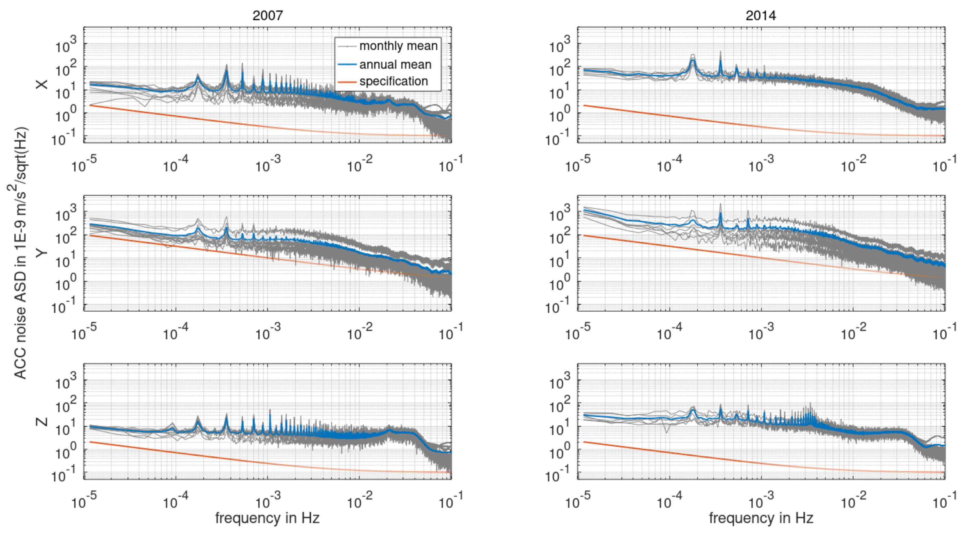
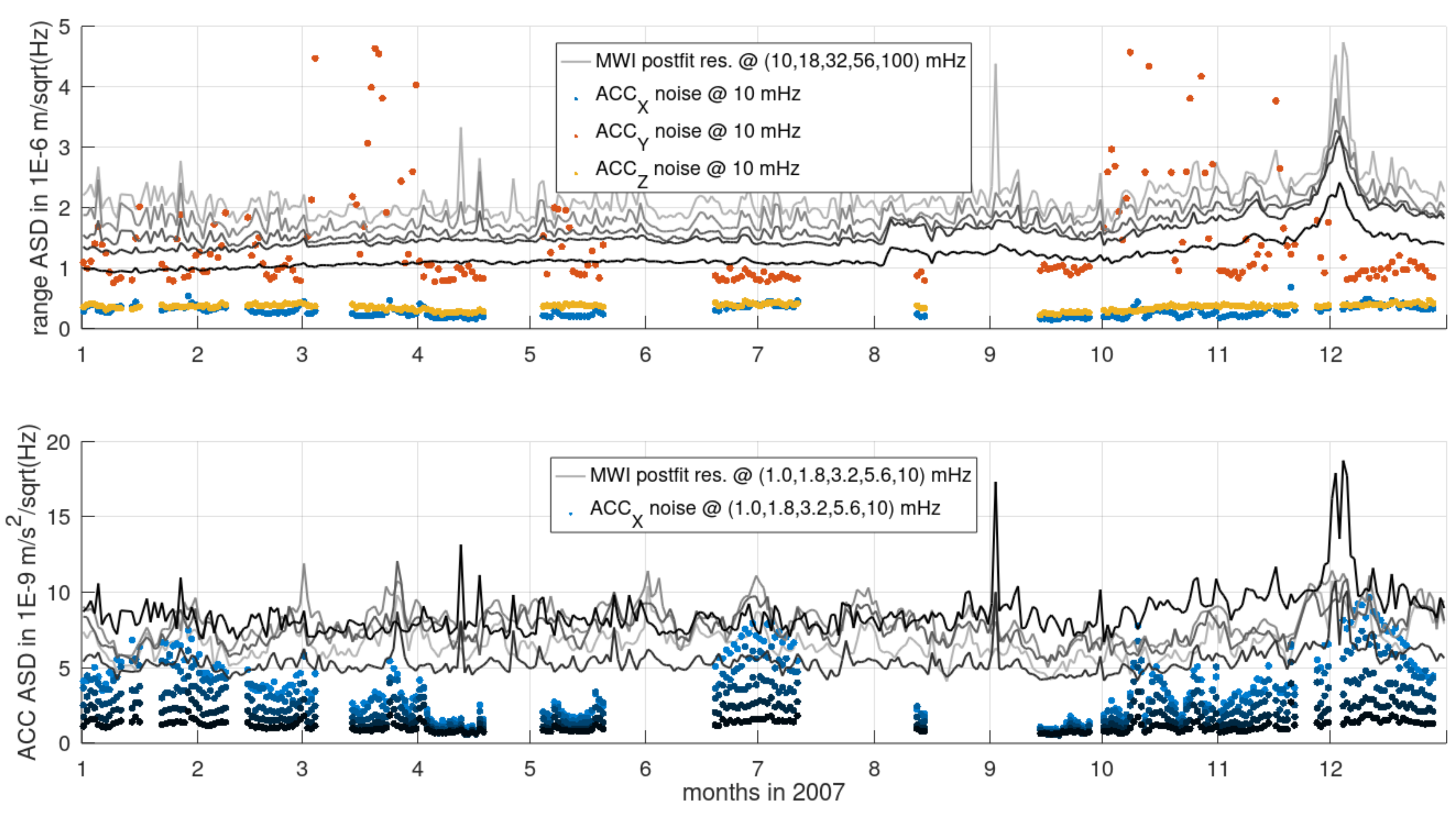
- ACC1B: 1 s sampling; ACC measurements in X (along-track), Z (radial) and Y (completes a right-handed system with X and Z, cross-track).
- GPS Navigation L1B (GNV1B): 5 s sampling; orbital positions of each satellite in an earth-fixed frame.
- Thruster L1B (THR1B): irregular sampling; contains time stamps and duration of thruster firings.
- Star Camera Assembly L1B (SCA1B): 5 s sampling; orientation of the satellites in terms of quaternions in an inertial frame.
- GNV1B and SCA1B sampling is increased using linear interpolation to match that of ACC1B. Then, the time shift that separates both satellites is determined based on the minimal distance of orbital positions. This time shift can then be applied to either satellite’s data products (with the respective sign). We applied it to those of satellite B.
- Data points contaminated by non-stochastic effects, i.e., thruster firings—the only deterministic error component provided in the L1B data—are removed. Although thruster firings may occur in a rapid sequence, each firing is generally short-periodic (well below one second). In the ACC Level-1A (L1A) data (raw 10.034 Hz ACC readings), they also appear as such. The processed ACC1B results from, amongst others, applying a 35 mHz filter to the L1A data. Therefore, these short pulses are smeared over periods of over 70 s (e.g., [27]). This error source is removed from the ACC1B data by cutting all data points in the range of 40 s to both sides of every thruster firing’s time stamp.
- ACC1B data, which are flagged with “proof mass voltage out of nominal range”, can be considered as irreversibly compromised and are, therefore, cut from the time series of both satellites. It is noted that within the frame of the analyses performed for this study, cutting data with other types of flags did not yield a better overall result.
- Remaining outliers in the ACC1B time series exceeding a 3-sigma criterion are removed.
- To achieve an optimal fit between the homogenized ACC1B-A/B time series, a least-squares adjustment was carried out where a scale factor and a six-parameter polynomial (bias, linear drift and periodic components of 1 and 2 Cycles Per Revolution (CPR)) was estimated daily for every ACC axis (cf. Equation (1)). Additionally, we considered the satellites’ relative orientations at their evaluated orbital positions (derived from SCA1B-A/B). It should be emphasized that we did not estimate the absolute bias, drift and scale but rather the relative values (i.e., one of the scale factors is fixed to 1). The observation equation for satellites A and B can be written as follows:
| relative scale factors (estimated daily) | |
| bias (estimated daily) | |
| linear drift (estimated daily) | |
| 1/2 CPR signal component scale factors (estimated daily) | |
| Rotation matrix (derived from SCA1B) | |
| ACC1B observations | |
| t | time |
| ω1 | angular velocity corresponding to 1 CPR |
2.2. Microwave Instrument
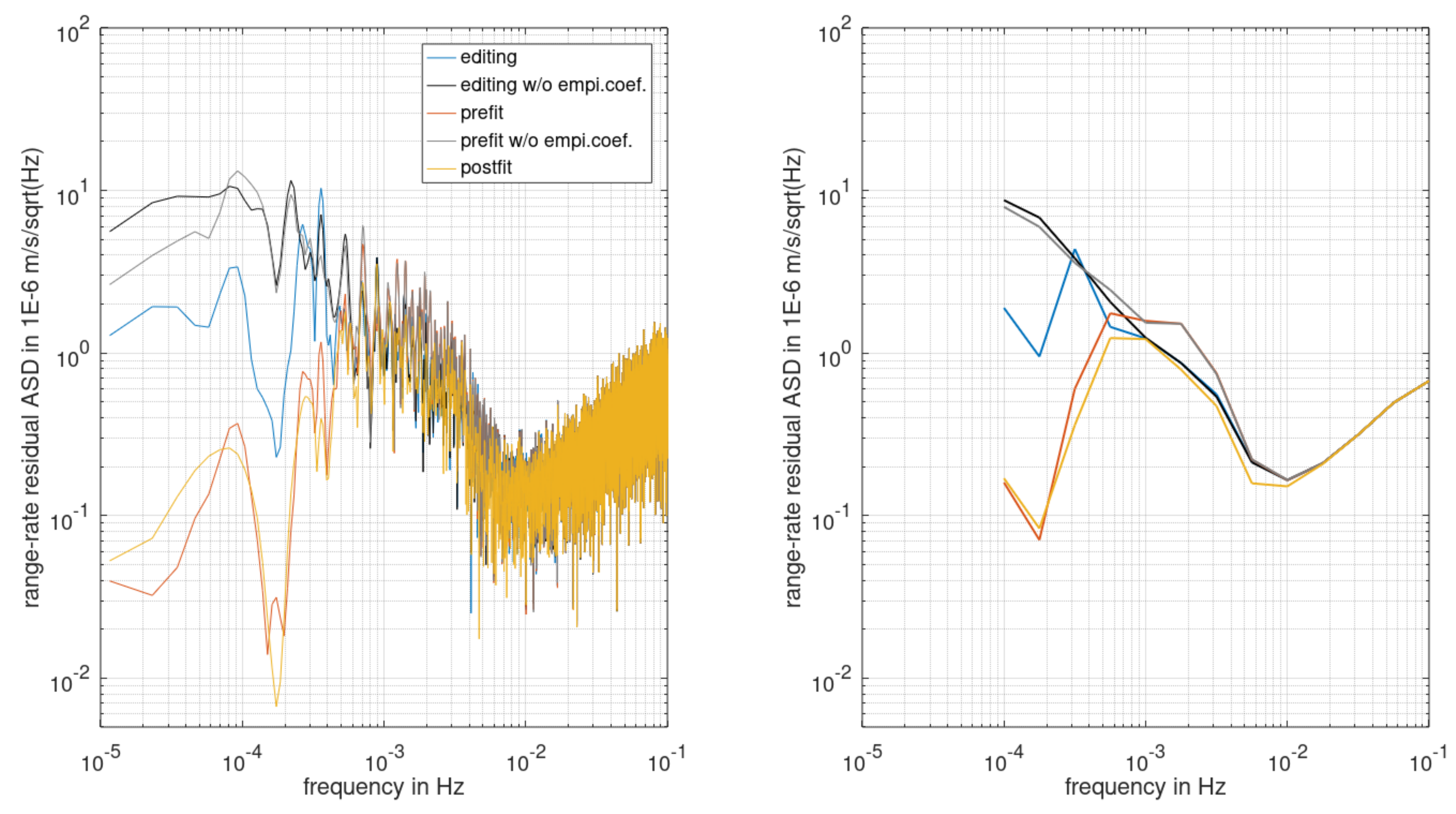
- “Editing residuals”: calculated before gravity field modeling and used for MWI data editing; L1B data reduced by an a priori static and time-variable gravity field signal and by other a priori signals, e.g., tidal signals.
- “Pre-fit residuals”: calculated after data editing and used for gravity field modeling; L1B data reduced by an a priori static gravity field signal and by other a priori signals, e.g., tidal signals (resulting in usually larger amplitudes than the editing residuals in the frequency band between 1 and 10 mHz).
- “Post-fit residuals”: calculated after gravity field modeling; L1B data reduced by all best-known estimated parameters.
3. Results
3.1. Accelerometers
3.2. Microwave Instrument

4. Impact on Gravity Field Retrieval Performance
| t | Time in years |
| K(t) + e(t) | SH coefficient time series with residuals |
| a | Constant parameter |
| b | Linear parameter |
| Cosine/Sine amplitudes of the annual/semi-annual signal. |
5. Conclusions
Author Contributions
Funding
Data Availability Statement
Conflicts of Interest
References
- Tapley, B.D.; Watkins, M.M.; Flechtner, F.; Reigber, C.; Bettadpur, S.; Rodell, M.; Sasgen, I.; Famiglietti, J.S.; Landerer, F.W.; Chambers, D.P.; et al. Contributions of GRACE to understanding climate change. Nat. Clim. Chang. 2019, 9, 358–369. [Google Scholar] [CrossRef] [PubMed]
- Longuevergne, L.; Scanlon, B.R.; Wilson, C.R. GRACE Hydrological estimates for small basins: Evaluating processing approaches on the High Plains Aquifer, USA. Water Resour. Res. 2010, 46, W11517. [Google Scholar] [CrossRef]
- Werth, S.; Güntner, A. Calibration of a Global Hydrological Model with GRACE Data. In System Earth via Geodetic-Geophysical Space Techniques; Springer: Berlin/Heidelberg, Germany, 2010; pp. 417–426. [Google Scholar] [CrossRef]
- Döll, P.; Schmied, H.M.; Schuh, C.; Portmann, F.T.; Eicker, A. Global-scale assessment of groundwater depletion and related groundwater abstractions: Combining hydrological modeling with information from well observations and GRACE satellites. Water Resour. Res. 2014, 50, 5698–5720. [Google Scholar] [CrossRef]
- Eicker, A.; Schumacher, M.; Kusche, J.; Döll, P.; Schmied, H.M. Calibration/Data Assimilation Approach for Integrating GRACE Data into the WaterGAP Global Hydrology Model (WGHM) Using an Ensemble Kalman Filter: First Results. Surv. Geophys. 2014, 35, 1285–1309. [Google Scholar] [CrossRef]
- Shepherd, A.; Ivins, E.R.; Geruo, A.; Barletta, V.R.; Bentley, M.J.; Bettadpur, S.; Briggs, K.H.; Bromwich, D.H.; Forsberg, R.; Galin, N.; et al. A Reconciled Estimate of Ice-Sheet Mass Balance. Science 2012, 338, 1183–1189. [Google Scholar] [CrossRef] [Green Version]
- Velicogna, I.; Sutterley, T.C.; van den Broeke, M.R. Regional acceleration in ice mass loss from Greenland and Antarctica using GRACE time-variable gravity data. Geophys. Res. Lett. 2014, 41, 8130–8137. [Google Scholar] [CrossRef] [Green Version]
- Humphrey, V.; Gudmundsson, L.; Seneviratne, S.I. A global reconstruction of climate-driven subdecadal water storage variability. Geophys. Res. Lett. 2017, 44, 2300–2309. [Google Scholar] [CrossRef]
- WMO. 2022. Available online: https://gcos.wmo.int/en/publications/gcos-implementation-plan2022 (accessed on 15 November 2022).
- Landerer, F.W.; Flechtner, F.M.; Save, H.; Webb, F.H.; Bandikova, T.; Bertiger, W.I.; Bettadpur, S.V.; Byun, S.H.; Dahle, C.; Dobslaw, H.; et al. Extending the Global Mass Change Data Record: GRACE Follow-On Instrument and Science Data Performance. Geophys. Res. Lett. 2020, 47, e2020GL088306. [Google Scholar] [CrossRef]
- Reigber, C. Gravity Field Recovery from Satellite Tracking Data. In Theory of Satellite Geodesy and Gravity Field Determination; Sanso, F., Rummel, R., Eds.; Springer: Berlin, Germany, 1989; Volume 25, pp. 197–234. [Google Scholar]
- Dahle, C.; Murböck, M.; Flechtner, F.; Dobslaw, H.; Michalak, G.; Neumayer, K.H.; Abrykosov, O.; Reinhold, A.; König, R.; Sulzbach, R.; et al. The GFZ GRACE RL06 Monthly Gravity Field Time Series: Processing Details and Quality Assessment. Remote. Sens. 2019, 11, 2116. [Google Scholar] [CrossRef]
- Save, H.; Bettadpur, S.; Tapley, B.D. High-resolution CSR GRACE RL05 mascons. J. Geophys. Res. Solid Earth 2016, 121, 7547–7569. [Google Scholar] [CrossRef]
- Watkins, M.M.; Wiese, D.N.; Yuan, D.-N.; Boening, C.; Landerer, F.W. Improved methods for observing Earth’s time variable mass distribution with GRACE using spherical cap mascons. J. Geophys. Res. Solid Earth 2015, 120, 2648–2671. [Google Scholar] [CrossRef]
- Kvas, A.; Behzadpour, S.; Ellmer, M.; Klinger, B.; Strasser, S.; Zehentner, N.; Mayer-Gürr, T. ITSG-Grace2018: Overview and Evaluation of a New GRACE-Only Gravity Field Time Series. J. Geophys. Res. Solid Earth 2019, 124, 9332–9344. [Google Scholar] [CrossRef] [Green Version]
- Kim, J. Simulation Study of a Low-Low Satellite-to-Satellite Tracking Mission; The University of Texas at Austin: Austin, TX, USA, 2000. [Google Scholar]
- Murböck, M.; Pail, R.; Daras, I.; Gruber, T. Optimal orbits for temporal gravity recovery regarding temporal aliasing. J. Geodesy 2013, 88, 113–126. [Google Scholar] [CrossRef]
- Flechtner, F.; Neumayer, K.-H.; Dahle, C.; Dobslaw, H.; Fagiolini, E.; Raimondo, J.-C.; Güntner, A. What Can be Expected from the GRACE-FO Laser Ranging Interferometer for Earth Science Applications. In Remote Sensing and Water Resources; Springer: Cham, Switzerland, 2016; pp. 263–280. [Google Scholar] [CrossRef] [Green Version]
- Daras, I.; Pail, R. Treatment of temporal aliasing effects in the context of next generation satellite gravimetry missions. J. Geophys. Res. Solid Earth 2017, 122, 7343–7362. [Google Scholar] [CrossRef]
- Ellmer, M. Contributions to GRACE Gravity Field Recovery: Improvements in Dynamic Orbit Integration Stochastic Modelling of the Antenna Offset Correction, and Co-Estimation of Satellite Orientations. Ph.D. Thesis, Graz University of Technology, Graz, Austria, 2018. [Google Scholar]
- Mayer-Gürr, T.; Behzadpour, S.; Ellmer, M.; Kvas, A.; Klinger, B.; Zehentner, N. ITSG-Grace2016—Monthly and Daily Gravity Field Solutions from GRACE. Data Publ. GFZ Data Serv. 2016. [Google Scholar] [CrossRef]
- Daras, I. Gravity Field Processing Towards Future LL-SST Satellite Missions. Doctoral Dissertation, Technische Universität München, Munich, Germany, 2016; pp. 23–39. [Google Scholar]
- Flury, J.; Bettadpur, S.; Tapley, B.D. Precise accelerometry onboard the GRACE gravity field satellite mission. Adv. Space Res. 2008, 42, 1414–1423. [Google Scholar] [CrossRef]
- Peterseim, N. TWANGS—High-Frequency Disturbing Signals in 10 Hz Accelerometer Data of the GRACE Satellites. Doctoral Dissertation, Technische Universität München, München, Germany, 2014. [Google Scholar]
- Klinger, B.; Mayer-Gürr, T. The role of accelerometer data calibration within GRACE gravity field recovery: Results from ITSG-Grace2016. Adv. Space Res. 2016, 58, 1597–1609. [Google Scholar] [CrossRef] [Green Version]
- Harvey, N.; McCullough, C.M.; Save, H. Modeling GRACE-FO accelerometer data for the version 04 release. Adv. Space Res. 2021, 69, 1393–1407. [Google Scholar] [CrossRef]
- Bandikova, T.; McCullough, C.; Kruizinga, G.L.; Save, H.; Christophe, B. GRACE accelerometer data transplant. Adv. Space Res. 2019, 64, 623–644. [Google Scholar] [CrossRef] [Green Version]
- Behzadpour, S.; Mayer-Gürr, T.; Krauss, S. GRACE Follow-On Accelerometer Data Recovery. J. Geophys. Res. Solid Earth 2021, 126, e2020JB021297. [Google Scholar] [CrossRef]
- Ditmar, P.; da Encarnação, J.T.; Farahani, H.H. Understanding data noise in gravity field recovery on the basis of inter-satellite ranging measurements acquired by the satellite gravimetry mission GRACE. J. Geodesy 2011, 86, 441–465. [Google Scholar] [CrossRef] [Green Version]
- Goswami, S.; Devaraju, B.; Weigelt, M.; Mayer-Gürr, T. Analysis of GRACE range-rate residuals with focus on KBR instrument system noise. Adv. Space Res. 2018, 62, 304–316. [Google Scholar] [CrossRef] [Green Version]
- Behzadpour, S.; Mayer-Gürr, T.; Flury, J.; Klinger, B.; Goswami, S. Multiresolution wavelet analysis applied to GRACE range-rate residuals. Geosci. Instrum. Methods Data Syst. 2019, 8, 197–207. [Google Scholar] [CrossRef] [Green Version]
- Müller, V.; Hauk, M.; Misfeldt, M.; Müller, L.; Wegener, H.; Yan, Y.; Heinzel, G. Comparing GRACE-FO KBR and LRI Ranging Data with Focus on Carrier Frequency Variations. Remote Sens. 2022, 14, 4335. [Google Scholar] [CrossRef]
- Touboul, P.; Willemenot, E.; Foulon, B.; Josselin, V. Accelerometers for CHAMP, GRACE and GOCE space missions: Synergy and evolution. Boll. Geof. Teor. Appl. 1999, 40, 321–327. [Google Scholar]
- Oppenheim, A.V.; Schafer, R.W. Digital signal processing (Book). In Research Supported by the Massachusetts Institute of Technology, Bell Telephone Laboratories, and Guggenheim Foundation; Prentice-Hall, Inc.: Englewood Cliffs, NJ, USA, 1975; 598p. [Google Scholar]
- Kornfeld, R.P.; Arnold, B.W.; Gross, M.A.; Dahya, N.T.; Klipstein, W.M.; Gath, P.F.; Bettadpur, S. GRACE-FO: The Gravity Recovery and Climate Experiment Follow-On Mission. J. Spacecr. Rocket. 2019, 56, 931–951. [Google Scholar] [CrossRef]
- Murböck, M. Virtual Constellations of Next Generation Gravity Missions. Doctoral Dissertation, Technische Universität München, München, Germany, 2015. [Google Scholar]
- Kvas, A.; Mayer-Gürr, T. GRACE gravity field recovery with background model uncertainties. J. Geodesy 2019, 93, 2543–2552. [Google Scholar] [CrossRef]


| ACCX | ACCY | ACCZ | MWI | |
|---|---|---|---|---|
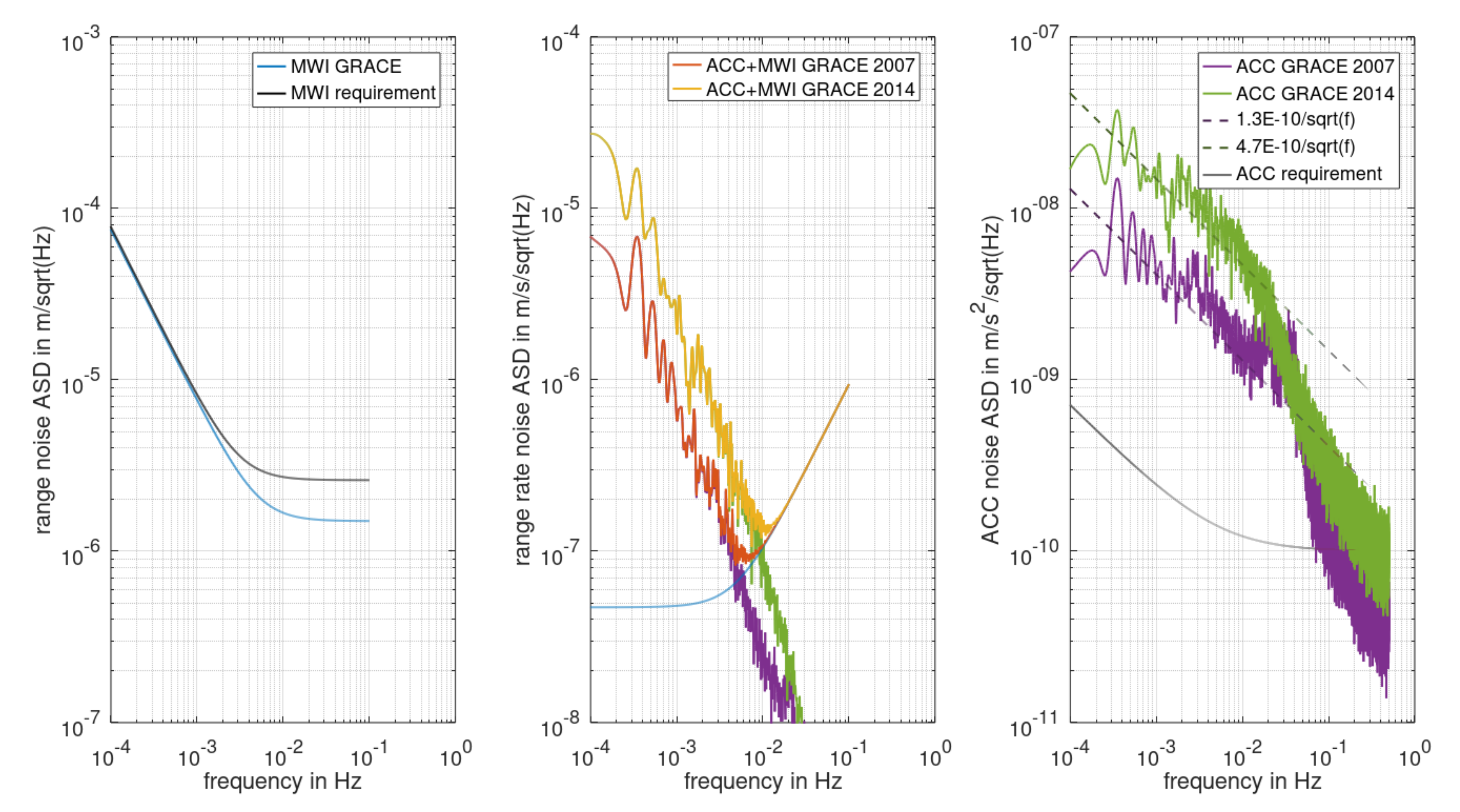
| 2007 | 1.3 | 8.2 | 1.0 | 1.7 |
| 2014 | 4.7 | 13 | 2.4 | 1.4 |
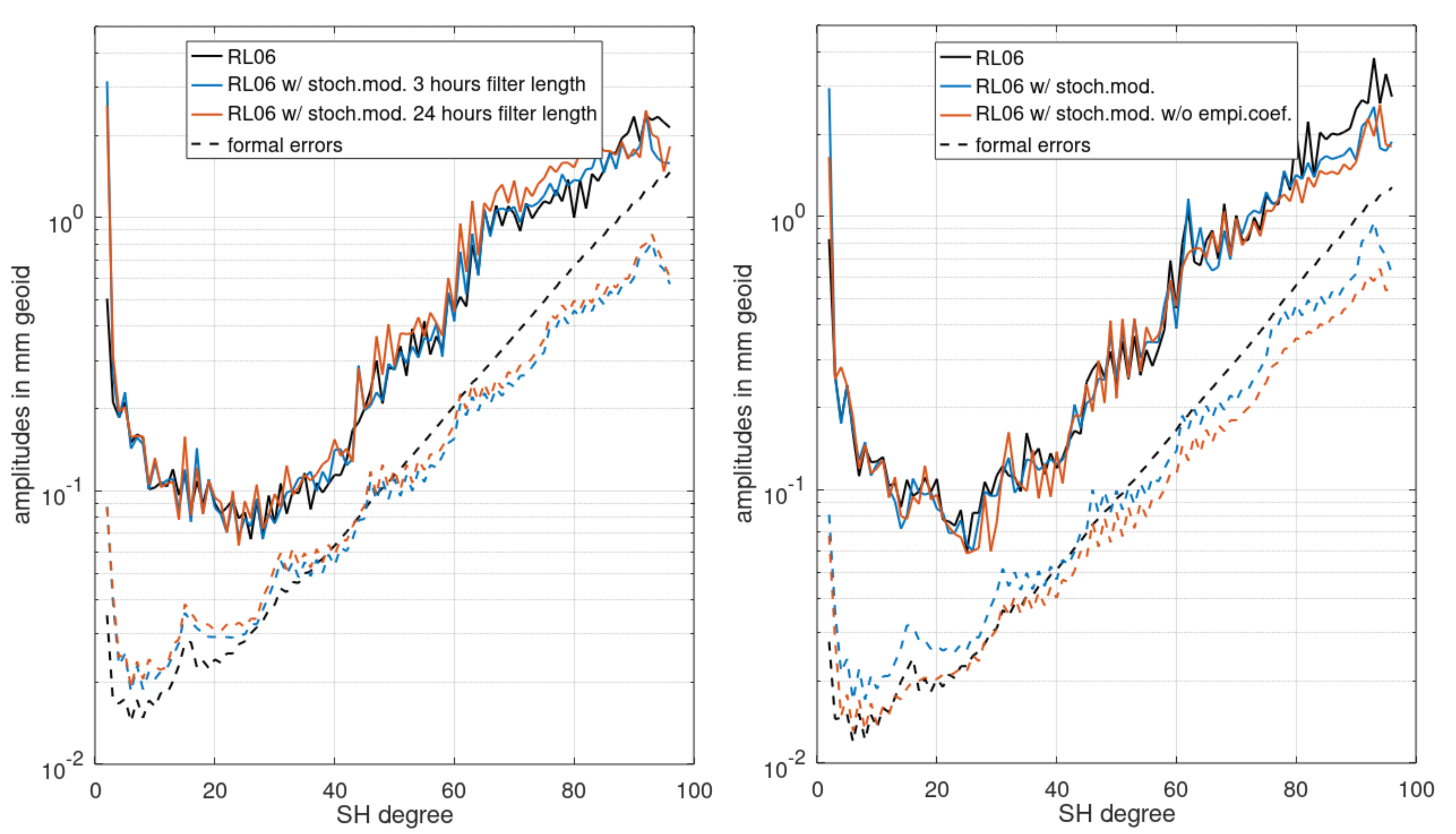
| Gauss. Radius in km | RL06 | RL06 w/stoch. Mod. | RL06 w/stoch. Mod. w/o empi.coef. |
|---|---|---|---|
| 500 | 1.4 | 1.9 | 1.4 |
| 450 | 1.6 | 2.0 | 1.6 |
| 400 | 2.0 | 2.3 | 2.0 |
| 350 | 2.8 | 3.0 | 2.7 |
| 300 | 4.8 | 4.7 | 4.5 |
| 250 | 10.7 | 9.7 | 9.3 |
Disclaimer/Publisher’s Note: The statements, opinions and data contained in all publications are solely those of the individual author(s) and contributor(s) and not of MDPI and/or the editor(s). MDPI and/or the editor(s) disclaim responsibility for any injury to people or property resulting from any ideas, methods, instructions or products referred to in the content. |
© 2023 by the authors. Licensee MDPI, Basel, Switzerland. This article is an open access article distributed under the terms and conditions of the Creative Commons Attribution (CC BY) license (https://creativecommons.org/licenses/by/4.0/).
Share and Cite
Murböck, M.; Abrykosov, P.; Dahle, C.; Hauk, M.; Pail, R.; Flechtner, F. In-Orbit Performance of the GRACE Accelerometers and Microwave Ranging Instrument. Remote Sens. 2023, 15, 563. https://doi.org/10.3390/rs15030563
Murböck M, Abrykosov P, Dahle C, Hauk M, Pail R, Flechtner F. In-Orbit Performance of the GRACE Accelerometers and Microwave Ranging Instrument. Remote Sensing. 2023; 15(3):563. https://doi.org/10.3390/rs15030563
Chicago/Turabian StyleMurböck, Michael, Petro Abrykosov, Christoph Dahle, Markus Hauk, Roland Pail, and Frank Flechtner. 2023. "In-Orbit Performance of the GRACE Accelerometers and Microwave Ranging Instrument" Remote Sensing 15, no. 3: 563. https://doi.org/10.3390/rs15030563