
Assessing Forest Landscape Stability through Automatic Identification of Landscape Pattern Evolution in Shanxi Province of China
Abstract
:1. Introduction
2. Materials and Methods
2.1. Study Area
2.2. Methodology
2.2.1. Data Preparation
2.2.2. Calculation of the Forest Landscape Index
2.2.3. Segmenting Time Series Based on TICC
2.2.4. Extracting Short-Term Change Process
2.2.5. Assessing Landscape Stability
3. Results
3.1. Characteristics of Subsequence in Landscape Dynamic
3.2. Spatiotemporal Distribution of the Forest Change Processes
3.3. Characteristics of Landscape Stability
3.4. Landscape Stability Assessment of Representative Regions
4. Discussion
- (1)
- Classification accuracy affected the landscape index calculation in landscape patterns. The results of landscape evolution modes based on this classification could be recognized as long as the annual classification accuracy was accepted since the recognition of landscape stability assessment is based on the change processes that have occurred in the landscape indices from the land cover maps.
- (2)
- A variety of driving factors and their interactions will affect ecological land degradation-restoration [53], and it is necessary to combine driving factors to understand the mechanism of forest landscape evolution. In the future, multiple time series can be constructed that consider different driving factors (such as drought, fire, and deforestation) to determine the relationship between forest landscape dynamics and driving factors.
- (3)
- The landscape change process defined in this study was not universal but based on prior knowledge and actual conditions in the study area. Such criteria may not apply to other land-use types [54,55,56,57,58,59]. Hence, future research must use deep-learning algorithms to detect change processes more intelligently to extract landscape evolution modes of various land-use types.
5. Conclusions
Author Contributions
Funding
Data Availability Statement
Acknowledgments
Conflicts of Interest
References
- Kang, W.; Liu, S.; Chen, X.; Feng, K.; Guo, Z.; Wang, T. Evaluation of ecosystem stability against climate changes via satellite data in the eastern sandy area of northern China. J. Environ. Manag. 2022, 308, 114596. [Google Scholar] [CrossRef]
- Sun, J.; Li, G.; Zhang, Y.; Qin, W.; Wang, M. Identification of priority areas for afforestation in the Loess Plateau region of China. Ecol. Indic. 2022, 140, 108998. [Google Scholar] [CrossRef]
- Cao, S.; Chen, L.; Yu, X. Impact of China’s Grain for Green Project on the landscape of vulnerable arid and semi-arid agricultural regions: A case study in northern Shaanxi Province. J. Appl. Ecol. 2009, 46, 536–543. [Google Scholar] [CrossRef]
- Chen, Y.; Wang, K.; Lin, Y.; Shi, W.; Song, Y.; He, X. Balancing green and grain trade. Nat. Geosci. 2015, 8, 739–741. [Google Scholar] [CrossRef]
- Xu, X.; Zhang, D. Evaluating the effect of ecological policies from the pattern change of persistent green patches–A case study of Yan’an in China’s Loess Plateau. Ecol. Inform. 2021, 63, 101305. [Google Scholar] [CrossRef]
- Cao, S.; Chen, L.; Shankman, D.; Wang, C.; Wang, X.; Zhang, H. Excessive reliance on afforestation in China’s arid and semi-arid regions: Lessons in ecological restoration. Earth-Science Rev. 2011, 104, 240–245. [Google Scholar] [CrossRef]
- Turner, M.G.; Romme, W.H.; Gardner, R.H.; O’Neill, R.V.; Kratz, T.K. A revised concept of landscape equilibrium: Disturbance and stability on scaled landscapes. Landsc. Ecol. 1993, 8, 213–227. [Google Scholar] [CrossRef]
- Amrutha, K.; Danumah, J.H.; Nikhil, S.; Saha, S.; Rajaneesh, A.; Mammen, P.C.; Ajin, R.S.; Kuriakose, S.L. Demarcation of Forest Fire Risk Zones in Silent Valley National Park and the Effectiveness of Forest Management Regime. J. Geovisualization Spat. Anal. 2022, 6, 8. [Google Scholar] [CrossRef]
- Raji, S.A.; Odunuga, S.; Fasona, M. Spatially Explicit Scenario Analysis of Habitat Quality in a Tropical Semi-arid Zone: Case Study of the Sokoto–Rima Basin. J. Geovisualization Spat. Anal. 2022, 6, 11. [Google Scholar] [CrossRef]
- Wu, J. Landscape sustainability science: Ecosystem services and human well-being in changing landscapes. Landsc. Ecol. 2013, 28, 999–1023. [Google Scholar] [CrossRef]
- Bai, B.; Tan, Y.; Guo, D.; Xu, B. Dynamic Monitoring of Forest Land in Fuling District Based on Multi-Source Time Series Remote Sensing Images. ISPRS Int. J. Geo-Inf. 2019, 8, 36. [Google Scholar] [CrossRef] [Green Version]
- Harris, A.; Carr, A.; Dash, J. Remote sensing of vegetation cover dynamics and resilience across southern Africa. Int. J. Appl. Earth Obs. Geoinf. 2013, 28, 131–139. [Google Scholar] [CrossRef]
- Liu, M.; Liu, X.; Wu, L.; Tang, Y.; Li, Y.; Zhang, Y.; Ye, L.; Zhang, B. Establishing forest resilience indicators in the hilly red soil region of southern China from vegetation greenness and landscape metrics using dense Landsat time series. Ecol. Indic. 2020, 121, 106985. [Google Scholar] [CrossRef]
- Duveneck, M.J.; Scheller, R.M. Measuring and managing resistance and resilience under climate change in northern Great Lake forests (USA). Landsc. Ecol. 2015, 31, 669–686. [Google Scholar] [CrossRef]
- Ma, J.; Zhang, C.; Guo, H.; Chen, W.; Yun, W.; Gao, L.; Wang, H. Analyzing Ecological Vulnerability and Vegetation Phenology Response Using NDVI Time Series Data and the BFAST Algorithm. Remote. Sens. 2020, 12, 3371. [Google Scholar] [CrossRef]
- von Keyserlingk, J.; de Hoop, M.; Mayor, A.; Dekker, S.; Rietkerk, M.; Foerster, S. Resilience of vegetation to drought: Studying the effect of grazing in a Mediterranean rangeland using satellite time series. Remote. Sens. Environ. 2021, 255, 112270. [Google Scholar] [CrossRef]
- Xu, W.; Wang, J.; Zhang, M.; Li, S. Construction of landscape ecological network based on landscape ecological risk assessment in a large-scale opencast coal mine area. J. Clean. Prod. 2020, 286, 125523. [Google Scholar] [CrossRef]
- Hu, W.; Wang, G. Advances in Research of Landscape Patterns and Ecological Processes of Wetland. Prog. Geogr. 2007, 22, 969–975. [Google Scholar]
- Hermosilla, T.; Wulder, M.; White, J.; Coops, N.C.; Pickell, P.D.; Bolton, D.K. Impact of time on interpretations of forest fragmentation: Three-decades of fragmentation dynamics over Canada. Remote. Sens. Environ. 2018, 222, 65–77. [Google Scholar] [CrossRef]
- Zhang, J.; Yang, X.; Wang, Z.; Zhang, T.; Liu, X. Remote Sensing Based Spatial-Temporal Monitoring of the Changes in Coastline Mangrove Forests in China over the Last 40 Years. Remote. Sens. 2021, 13, 1986. [Google Scholar] [CrossRef]
- Kennedy, R.E.; Yang, Z.; Cohen, W.B. Detecting trends in forest disturbance and recovery using yearly Landsat time series: 1. LandTrendr—Temporal segmentation algorithms. Remote Sens. Environ. 2010, 114, 2897–2910. [Google Scholar] [CrossRef]
- Huang, C.; Goward, S.N.; Masek, J.G.; Thomas, N.; Zhu, Z.; Vogelmann, J.E. An automated approach for reconstructing recent forest disturbance history using dense Landsat time series stacks. Remote Sens. Environ. 2010, 114, 183–198. [Google Scholar] [CrossRef]
- Lhermitte, S.; Verbesselt, J.; Verstraeten, W.; Coppin, P. A comparison of time series similarity measures for classification and change detection of ecosystem dynamics. Remote. Sens. Environ. 2011, 115, 3129–3152. [Google Scholar] [CrossRef]
- Verbesselt, J.; Hyndman, R.; Newnham, G.; Culvenor, D. Detecting trend and seasonal changes in satellite image time series. Remote Sens. Environ. 2010, 114, 106–115. [Google Scholar] [CrossRef]
- Prokopová, M.; Salvati, L.; Egidi, G.; Cudlín, O.; Včeláková, R.; Plch, R.; Cudlín, P. Envisioning Present and Future Land-Use Change under Varying Ecological Regimes and Their Influence on Landscape Stability. Sustainability 2019, 11, 4654. [Google Scholar] [CrossRef] [Green Version]
- Lele, N.; Nagendra, H.; Southworth, J. Accessibility, Demography and Protection: Drivers of Forest Stability and Change at Multiple Scales in the Cauvery Basin, India. Remote. Sens. 2010, 2, 306–332. [Google Scholar] [CrossRef] [Green Version]
- Zhang, X.; Wang, G.; Xue, B.; Zhang, M.; Tan, Z. Dynamic landscapes and the driving forces in the Yellow River Delta wetland region in the past four decades. Sci. Total. Environ. 2021, 787, 147644. [Google Scholar] [CrossRef] [PubMed]
- Jaeger, J.A.G. Landscape division, splitting index, and effective mesh size: New measures of landscape fragmentation. Landsc. Ecol. 2000, 15, 115–130. [Google Scholar] [CrossRef]
- Wang, Y.; Brandt, M.; Zhao, M.; Xing, K.; Wang, L.; Tong, X.; Xue, F.; Kang, M.; Jiang, Y.; Fensholt, R. Do afforestation projects increase core forests? Evidence from the Chinese Loess Plateau. Ecol. Indic. 2020, 117, 106558. [Google Scholar] [CrossRef]
- Zhang, Y.; Liu, X.; Yang, Q.; Liu, Z.; Li, Y. Extracting Frequent Sequential Patterns of Forest Landscape Dynamics in Fenhe River Basin, Northern China, from Landsat Time Series to Evaluate Landscape Stability. Remote. Sens. 2021, 13, 3963. [Google Scholar] [CrossRef]
- Chazdon, R.L.; Brancalion, P.H.S.; Laestadius, L.; Bennett-Curry, A.; Buckingham, K.; Kumar, C.; Moll-Rocek, J.; Vieira, I.C.G.; Wilson, S.J. When is a forest a forest? Forest concepts and definitions in the era of forest and landscape restoration. AMBIO 2016, 45, 538–550. [Google Scholar] [CrossRef] [PubMed]
- Qiu, B.; Chen, G.; Tang, Z.; Lu, D.; Wang, Z.; Chen, C. Assessing the Three-North Shelter Forest Program in China by a novel framework for characterizing vegetation changes. ISPRS J. Photogramm. Remote Sens. 2017, 133, 75–88. [Google Scholar] [CrossRef]
- Liu, S.; Gong, P. Change of surface cover greenness in China between 2000 and 2010. Chin. Sci. Bull. 2012, 57, 2835–2845. [Google Scholar] [CrossRef] [Green Version]
- Li, Y.; Cao, Z.; Long, H.; Liu, Y.; Li, W. Dynamic analysis of ecological environment combined with land cover and NDVI changes and implications for sustainable urban–rural development: The case of Mu Us Sandy Land, China. J. Clean. Prod. 2017, 142, 697–715. [Google Scholar] [CrossRef]
- Forzieri, G.; Dakos, V.; McDowell, N.G.; Ramdane, A.; Cescatti, A. Emerging signals of declining forest resilience under climate change. Nature 2022, 608, 534–539. [Google Scholar] [CrossRef]
- Jian, M.; Wang, J.; Yu, H.; Wang, G.-G. Integrating object proposal with attention networks for video saliency detection. Inf. Sci. 2021, 576, 819–830. [Google Scholar] [CrossRef]
- Hallac, D.; Vare, S.; Boyd, S.; Leskovec, J. Toeplitz Inverse Covariance-Based Clustering of Multivariate Time Series Data. In Proceedings of the 23rd ACM SIGKDD International Conference on Knowledge Discovery and Data Mining, Halifax, NS, Canada, 13–17 August 2017; pp. 215–223. [Google Scholar]
- Miao, Z.; Marrs, R. Ecological restoration and land reclamation in open-cast mines in Shanxi Province, China. J. Environ. Manag. 2000, 59, 205–215. [Google Scholar] [CrossRef]
- Yan, D.; Bai, Z.; Liu, X. Heavy-Metal Pollution Characteristics and Influencing Factors in Agricultural Soils: Evidence from Shuozhou City, Shanxi Province, China. Sustainability 2020, 12, 1907. [Google Scholar] [CrossRef] [Green Version]
- Gu, L.; Gong, Z.; Du, Y. Evolution characteristics and simulation prediction of forest and grass landscape fragmentation based on the “Grain for Green” projects on the Loess Plateau, P.R. China. Ecol. Indic. 2021, 131, 108240. [Google Scholar] [CrossRef]
- Li, S.; Liang, W.; Fu, B.; Lü, Y.; Fu, S.; Wang, S.; Su, H. Vegetation changes in recent large-scale ecological restoration projects and subsequent impact on water resources in China’s Loess Plateau. Sci. Total. Environ. 2016, 569–570, 1032–1039. [Google Scholar] [CrossRef]
- Feng, R.; Wang, F.; Wang, K. Spatial-temporal patterns and influencing factors of ecological land degradation-restoration in Guangdong-Hong Kong-Macao Greater Bay Area. Sci. Total. Environ. 2021, 794, 148671. [Google Scholar] [CrossRef] [PubMed]
- Wulder, M.A.; White, J.C.; Han, T.; Coops, N.C.; Cardille, J.A.; Holland, T.; Grills, D. Monitoring Canada’s forests. Part 2: National forest fragmentation and pattern. Can. J. Remote. Sens. 2008, 34, 563–584. [Google Scholar] [CrossRef]
- Zhao, Y.; He, C.; Zhang, Q. Monitoring vegetation dynamics by coupling linear trend analysis with change vector analysis: A case study in the Xilingol steppe in northern China. Int. J. Remote. Sens. 2011, 33, 287–308. [Google Scholar] [CrossRef]
- Li, F.; Cheng, C.; Yang, R. A review of ecosystem restoration: Progress and prospects of domestic and abroad. Biodivers. Sci. 2022, 30, 22519. [Google Scholar] [CrossRef]
- Zhou, G.; Liu, S.; Li, Z.; Zhang, D.; Tang, X.; Zhou, C.; Yan, J.; Mo, J. Old-Growth Forests Can Accumulate Carbon in Soils. Science 2006, 314, 1417. [Google Scholar] [CrossRef] [PubMed] [Green Version]
- Barlow, J.; Gardner, T.A.; Araujo, I.S.; Ávila-Pires, T.C.; Bonaldo, A.B.; Costa, J.E.; Esposito, M.C.; Ferreira, L.V.; Hawes, J.; Hernandez, M.I.M.; et al. Quantifying the biodiversity value of tropical primary, secondary, and plantation forests. Proc. Natl. Acad. Sci. USA 2007, 104, 18555–18560. [Google Scholar] [CrossRef] [PubMed] [Green Version]
- Wingfield, M.J.; Brockerhoff, E.G.; Wingfield, B.D.; Slippers, B. Planted forest health: The need for a global strategy. Science 2015, 349, 832–836. [Google Scholar] [CrossRef]
- McGarigal, K.; McComb, W.C. Relationships Between Landscape Structure and Breeding Birds in the Oregon Coast Range. Ecol. Monogr. 1995, 65, 235–260. [Google Scholar] [CrossRef] [Green Version]
- Li, Y.; Liu, M.; Liu, X.; Yang, W.; Wang, W. Characterising three decades of evolution of forest spatial pattern in a major coal-energy province in northern China using annual Landsat time series. Int. J. Appl. Earth Obs. Geoinf. 2020, 95, 102254. [Google Scholar] [CrossRef]
- Oikonomakis, N.; Ganatsas, P. Land cover changes and forest succession trends in a site of Natura 2000 network (Elatia forest), in northern Greece. For. Ecol. Manag. 2012, 285, 153–163. [Google Scholar] [CrossRef]
- Zhao, Y. Research of Regionalism by Ecological Fragility Based on Condition of Soil Erosion in Shanxi Province. J. Soil. Water Conserv. 2003, 17, 71–74. [Google Scholar] [CrossRef]
- Sun, B.; Li, Z.; Gao, W.; Zhang, Y.; Gao, Z.; Song, Z.; Qin, P.; Tian, X. Identification and assessment of the factors driving vegetation degradation/regeneration in drylands using synthetic high spatiotemporal remote sensing Data—A case study in Zhenglanqi, Inner Mongolia, China. Ecol. Indic. 2019, 107, 105614. [Google Scholar] [CrossRef]
- Tian, L.; Liu, X.; Liu, M.; Wu, L. State-and-Evolution Detection Models: A Framework for Continuously Monitoring Landscape Pattern Change. IEEE Trans. Geosci. Remote. Sens. 2021, 60, 1–14. [Google Scholar] [CrossRef]
- Coops, N.C.; Gillanders, S.N.; Wulder, M.A.; Gergel, S.E.; Nelson, T.; Goodwin, N.R. Assessing changes in forest fragmentation following infestation using time series Landsat imagery. For. Ecol. Manag. 2010, 259, 2355–2365. [Google Scholar] [CrossRef]
- Cui, H.; Liu, M.; Chen, C. Ecological Restoration Strategies for the Topography of Loess Plateau Based on Adaptive Ecological Sensitivity Evaluation: A Case Study in Lanzhou, China. Sustainability 2022, 14, 2858. [Google Scholar] [CrossRef]
- Chen, L.; Sun, R.; Lu, Y. A conceptual model for a process-oriented landscape pattern analysis. Sci. China Earth Sci. 2019, 62, 2050–2057. [Google Scholar] [CrossRef]
- Chowdhury, S.; Peddle, D.R.; Wulder, M.A.; Heckbert, S.; Shipman, T.C.; Chao, D.K. Estimation of land-use/land-cover changes associated with energy footprints and other disturbance agents in the Upper Peace Region of Alberta Canada from 1985 to 2015 using Landsat data. Int. J. Appl. Earth Obs. Geoinf. 2021, 94, 102224. [Google Scholar] [CrossRef]
- Cardille, J.; Turner, M.; Clayton, M.; Gergel, S.; Price, S. METALAND: Characterizing Spatial Patterns and Statistical Context of Landscape Metrics. Bioscience 2005, 55, 983–988. [Google Scholar] [CrossRef]


| Index | Formula | Units | Ecological Significance |
|---|---|---|---|
| Forest cover area (CA) | CA = F() F:total forest area in landscape units () | ha | Forest area is the basis for maintaining forest ecosystem activities. The loss of forest represents the loss of biological habitat, which translates into reduced stability. The trend in CA is also an important basis for distinguishing different ecological processes. |
| Patch density (PD) | PD = N: number of patches in landscape units A: area of landscape units (1 ) | number (1 ) | PD can reflect forest fragmentation, which is the most direct manifestation of forest landscape structural changes and is an important indicator to measure the activity of ecological processes. The increase in fragmentation often represents a decrease in stability. |
| Change Process | Trend | Ecological Significance | |
|---|---|---|---|
| CA | PD | ||
| Degradation | Negative | No trend | The decrease in the area of forest patches does not change the overall fragmentation, and the patches disappear from locations on the edges or inside of existing patches. Patch changes correspond to the change process of shrinkage and perforation. |
| Degradation | Negative | Negative | Decreased area of forest patches leads to decreased overall fragmentation. Patch changes correspond to the change process of attrition. |
| Degradation | Negative | Positive | Decrease in patch area fragments forest patches, leading to an increase in overall fragmentation. Patch changes correspond to the change process of division. |
| Degradation | No trend | Positive | Although the patch area is stable, the degree of fragmentation increases and the integrity of the forest landscape decreases, which is considered degradation. |
| Restoration | Positive | No trend | Increase in patch area does not affect overall fragmentation; the increase in patch area is located at the edge or inside of the patches. Patch changes correspond to the change processes of expansion and infilling. |
| Restoration | Positive | Positive | An increase in the number of patches leads to an increase in forest area and fragmentation. Patch changes correspond to the change process of outlying. |
| Restoration | Positive | Negative | Increase in the patch area reduces overall fragmentation. This is the process of landscape connectivity. |
| Restoration | No trend | Negative | Patch area is stable, and the decrease in fragmentation implies that the integrity of the forest landscape has increased, which is considered restoration. |
| Stable | No trend | No trend | Both the area and the fragmentation remain stable. |
| Long-Term Evolution Mode | Description | Stability Measurement |
|---|---|---|
| No Change mode | There are no restoration or degradation processes in long-term evolution. Forest landscape pattern does not change. | Stable |
| Decrease mode | There are at least one or more degradation processes but no restoration process in long-term evolution. | Unstable |
| Increase mode | There are at least one or more restoration processes but no degradation processes in long-term evolution. | Stable |
| Wave mode | There are both degradation and restoration processes in long-term evolution. For example, forest landscape patterns may first degrade, then recover to stable. | Cumulative time switching frequency restoration time |
| Index | Number of Clusters | ||||||
|---|---|---|---|---|---|---|---|
| 6 | 7 | 8 | 9 | 10 | 11 | 12 | |
| BIC () | 5.791 | 5.966 | 6.131 | 5.804 | 7.163 | 7.474 | 8.017 |
| DBI | 1.72 | 1.92 | 1.94 | 1.60 | 2.03 | 2.00 | 2.28 |
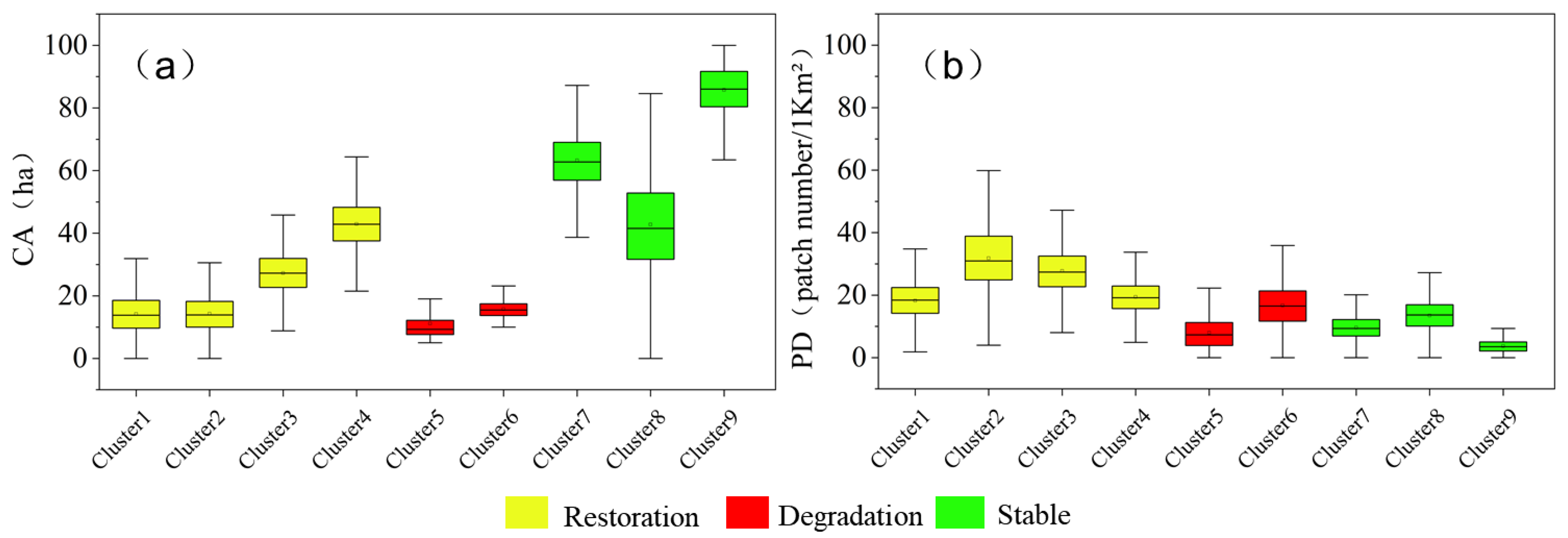
| Cluster | CA (ha) | PD (Patch Number/1 Km2) | Change Process | ||||||
|---|---|---|---|---|---|---|---|---|---|
| Mean | Change Rate | St.dv | Trend | Mean | Change Rate | St.dv | Trend | ||
| 1 | 14.1 | 0.59 | 6.7 | Positive | 18.2 | −0.40 | 5.9 | Negative | Restoration |
| 2 | 14.2 | 0.64 | 6.0 | Positive | 31.8 | 1.66 | 10.5 | Positive | Restoration |
| 3 | 27.2 | 0.44 | 7.0 | Positive | 27.7 | 0.37 | 7.2 | Positive | Restoration |
| 4 | 42.9 | 0.38 | 8.0 | Positive | 19.4 | −0.02 | 5.4 | No trend | Restoration |
| 5 | 11.1 | −0.54 | 5.1 | Negative | 7.9 | −0.23 | 5.1 | Negative | Degradation |
| 6 | 15.7 | −0.75 | 2.9 | Negative | 16.7 | 0.57 | 7.1 | Positive | Degradation |
| 7 | 63.2 | 0.06 | 9.2 | No trend | 9.5 | −0.05 | 3.8 | No trend | Stable |
| 8 | 42.7 | 0.12 | 15.3 | No trend | 13.4 | 0.08 | 5.1 | No trend | Stable |
| 9 | 85.7 | 0.04 | 7.7 | No trend | 3.6 | −0.07 | 2.0 | No trend | Stable |
Disclaimer/Publisher’s Note: The statements, opinions and data contained in all publications are solely those of the individual author(s) and contributor(s) and not of MDPI and/or the editor(s). MDPI and/or the editor(s) disclaim responsibility for any injury to people or property resulting from any ideas, methods, instructions or products referred to in the content. |
© 2023 by the authors. Licensee MDPI, Basel, Switzerland. This article is an open access article distributed under the terms and conditions of the Creative Commons Attribution (CC BY) license (https://creativecommons.org/licenses/by/4.0/).
Share and Cite
Hou, B.; Wei, C.; Liu, X.; Meng, Y.; Li, X. Assessing Forest Landscape Stability through Automatic Identification of Landscape Pattern Evolution in Shanxi Province of China. Remote Sens. 2023, 15, 545. https://doi.org/10.3390/rs15030545
Hou B, Wei C, Liu X, Meng Y, Li X. Assessing Forest Landscape Stability through Automatic Identification of Landscape Pattern Evolution in Shanxi Province of China. Remote Sensing. 2023; 15(3):545. https://doi.org/10.3390/rs15030545
Chicago/Turabian StyleHou, Bowen, Caiyong Wei, Xiangnan Liu, Yuanyuan Meng, and Xiaoyue Li. 2023. "Assessing Forest Landscape Stability through Automatic Identification of Landscape Pattern Evolution in Shanxi Province of China" Remote Sensing 15, no. 3: 545. https://doi.org/10.3390/rs15030545