Article

Analysis of Depths Derived by Airborne Lidar and Satellite Imaging to Support Bathymetric Mapping Efforts with Varying Environmental Conditions: Lower Laguna Madre, Gulf of Mexico

1
Near Surface Observatory, Bureau of Economic Geology, John A. and Katherine G. Jackson School of Geosciences, The University of Texas at Austin, Austin, TX 78758, USA
2
Shallow Water Earth Observation Laboratory, Department of Geography, Environment and Geomatics, University of Ottawa, Ottawa, ON K1N 6N5, Canada
*
Author to whom correspondence should be addressed.
Remote Sens. 2023, 15(24), 5754; https://doi.org/10.3390/rs15245754
Submission received: 6 October 2023 / Revised: 10 December 2023 / Accepted: 12 December 2023 / Published: 16 December 2023

Abstract

:
In 2017, Bureau of Economic Geology (BEG) researchers at the University of Texas at Austin (UT Austin) conducted an airborne lidar survey campaign, collecting topographic and bathymetric data over Lower Laguna Madre, which is a shallow hypersaline lagoon in south Texas. Researchers acquired 60 hours of lidar data, covering an area of 1600 km2 with varying environmental conditions influencing water quality and surface heights. In the southernmost parts of the lagoon, in-situ measurements were collected from a boat to quantify turbidity, water transparency, and depths. Data analysis included processing of Sentinel-2 L1C satellite imagery pixel reflectance to classify locations with intermittent turbidity. Lidar measurements were compared to sonar recordings, and results revealed height differences of 5–25 cm where the lagoon was shallower than 3.35 m. Further, researchers analyzed satellite bathymetry at relatively transparent lagoon locations, and the results produced height agreement within 13 cm. The study concluded that bathymetric efforts with airborne lidar and optical satellite imaging have practical limitations and comparable results in large and dynamic shallow coastal estuaries, where in-situ measurements and tide adjustments are essential for height comparisons.

1. Introduction

Remote sensing is the science of gathering information about an object without physical contact. In recent years, the use of active remote sensing technologies from different platforms (orbiting satellites, aircraft, or Unmanned Airborne Vehicles) has become increasingly popular to measure the topography of hard surfaces [1,2] or the depths of shallow and relatively transparent waters [3,4]. As a result, several projects investigated and used the technology for coastal applications such as shoreline mapping, erosion, and change detection [5,6,7,8].
In dynamic coastal and fluvial inland water reservoirs, it is challenging to measure depths because of electromagnetic energy (EM) scattering from the water surface and the rapid amplitude degradation in the water column. A number of studies revealed the challenges of bottom mapping with varying levels of water quality in coastal and inland waters using satellite imaging and measuring pixel reflectance [9,10,11]. However, only a few investigated the combined use of airborne lidar and satellite imaging technologies. For instance, Ji et al. introduced a feature-based data fusion model [12], and Yeu et al. evaluated and enhanced the accuracy of satellite altimeter bathymetry using airborne lidar and multi-beam sonar on transparent, coastal waters of western Korea using a gravity-geologic model [13].
In 2017, the Bureau of Economic Geology (BEG) at The University of Texas at Austin (UT Austin) acquired topographic and bathymetric airborne lidar data over Lower Laguna Madre, a hypersaline lagoon in south Texas. Previously, using an airborne lidar system, BEG researchers completed projects on the Gulf Coast, mapping the shallow seafloor along the Gulf of Mexico and the Pacific Coast [7] and investigating bottom morphologies along various river sheds in the southern US [14,15]. The principal research motivation was to investigate the feasibility of measuring the lagoon bottom with airborne lidar and quantify lidar bathymetry’s accuracy with applicable survey and in-situ methods. We need to emphasize that remote sensing methods used in this study are familiar; however, their application in challenging and varying coastal environments to complement and validate each other is essentially important to the remote sensing community and has not been studied or documented in detail.
For this purpose, we prepared a ground control surface, collected dual-frequency sonar readings, observed transparency with a Secchi disk, and sampled turbidity in nephelometric measurements from a boat. Furthermore, we studied satellite imaging pixel reflectance and conducted satellite-derived bathymetry (SDB).
We aimed to address the following research questions in detail:
  • Can we measure the bottom of a shallow and hypersaline lagoon using an airborne lidar system? What were the possible operational bottlenecks, and what lessons did we learn?
  • Can we confirm the accuracy of lidar bathymetry with sonar? How do they complement each other?
  • How can we predict varying levels of turbidity based on satellite imaging? What were the potential benefits of conducting quantitative pixel reflectance analysis in bathymetric lidar mapping?
  • Is SDB a feasible methodology to measure the depths of shallow, turbid, and hypersaline lagoons? Can we compare and quantify SDB to lidar bathymetry in these conditions?

2. Materials and Methods

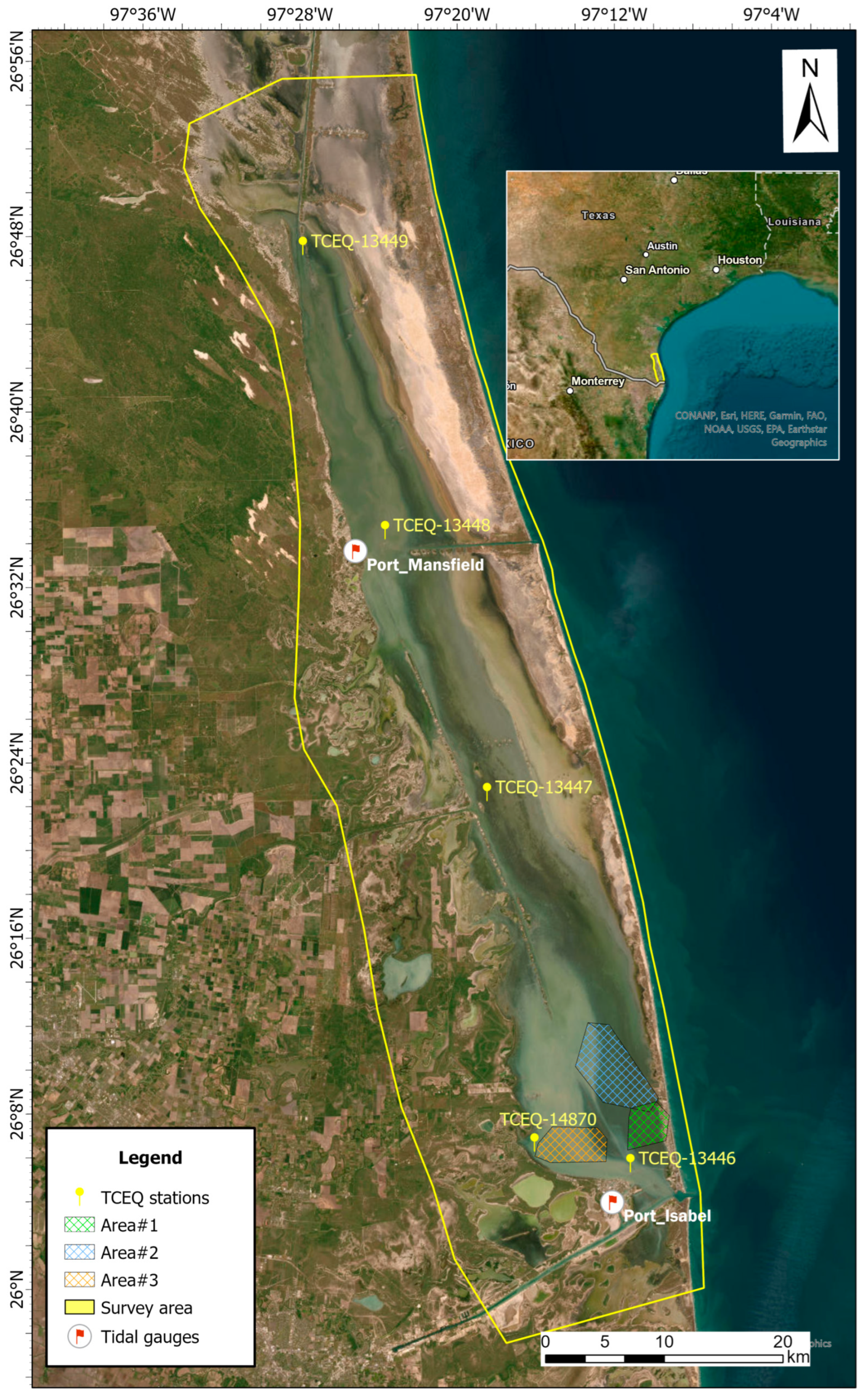
2.1. Project Location

In Texas, Lower Laguna Madre is a hypersaline (i.e., saltier than seawater) lagoon that is physio-graphically divided into two subunits [16]. Upper Laguna Madre is separated from the lower section by a canal and partial land bridge, which was constructed from dredged material during the building of the Gulf Intracoastal Waterway [17]. To the south, Lower Laguna Madre borders Mexico and covers an area larger than 800 km2 (310 mi2). The lagoon waters are transparent and shallow in the southeast and northern sections, and water quality changes with northerly winds that carry sedimentation from sand dunes and discharge freshwater streams. The lagoon has a unique seagrass ecosystem, protected by the Atascosa National Wildlife Refuge area in the north and by Padre Island on the Gulf Coast. Here, seagrass beds serve as essential nursery areas for various Gulf of Mexico species, such as supplying food and shelter for Redhead Ducks (Aytha americana). Because of seagrass’ essential role in supporting fish and wildlife resources, studies have attempted to map the lagoon using remote sensing technologies [18,19].

2.2. In-Situ Campaign

In 2017, an in-situ campaign was conducted in three distinct areas clustered in the southern portion of the lagoon, where it was possible to observe water transparency, depth, and turbidity (Appendix A). We sampled water with a turbidimeter and measured transparency with a Secchi disk. In the north, access to the lagoon was restricted due to private lands and the absence of public roads. We observed that in-situ Area-1 was shallow, transparent, and registered the least amount of turbidity content, in-situ Area-2 had varying turbidity and transparency, and in-situ Area-3 recorded the highest turbidity concentration (Figure 1a,b).
We completed the sonar surveys on three dates where atmospheric conditions influencing the lagoon conditions were similar: calm and no precipitation. Survey dates 01/05 (Area-1), 05/05 (Area-2), and 12/05 (Area-3) were executed coincidently with airborne lidar data acquisition, and depths were measured using a dual-frequency, single-beam sonar. We mounted the sonar unit onto a kayak and towed it throughout the lagoon with a power boat with an onboard observer. The sonar transducer was submerged with the operator in the kayak, and the resulting 6 cm was added to the recorded heights. The sonar measured the lagoon bottom every two seconds, and the observer manually triggered the unit (waypoints) various times at each specified location where additional turbidity and water transparency measurements were sampled.
The sonar unit was calibrated in the lab environment, in the freshwater tank (UT Austin, Advanced Research Laboratories), producing depth measurements with a standard deviation of 2.7 cm at 11.8 m depth, which is acceptable for shallow-classified airborne lidar mapping systems [20]. In salt waters, sound waves propagate faster and require additional adjustment for salinity (S), water temperature (T), and depth (z). In Lower Laguna Madre, the typical salinity is 35.3 parts per thousand (ppt) [21], and we confirmed this value with the Texas Commission on Environmental Quality (TCEQ) stations (IDs: 13446 and 13447). These stations reported an average of 36.1 ppt and 38.6 ppt for all 2017 samplings. Figure 2 illustrates the survey location, in-situ areas, tide gauges, and TCEQ reference stations.
We recorded the water temperature using the sonar transducer, where the mean temperature varied (24.7, 23.4, and 26.2 °C), depending on the location and the survey day. Because the depth varied at each in-situ location, we used the mean value in the empirical formula (Equation (1)) to calculate the speed of sound in the water using coefficients (a1an) [22]. Computations revealed that sound waves propagated with different velocities for each survey day (1533.9, 1530.7, and 1537.5 m/s) in Lower Laguna Madre, which required an adjustment of 1/0.963–0.967 for sonar readings. Because the lagoon was calm and shallow, and the rocking movement with the kayak was minimal, we did not consider rotational adjustment (attitude) of sonar readings. However, because 10 degrees of boat roll would equal 3 cm of additional ranging in a 2 m water column, we recommend an inertial movement unit (IMU) sensor integration for rotational adjustment of sonar recordings in deeper and choppier waters.
c T ,   S ,   z = a 1 + a 2 T + a 3 T 2 + a 4 T 3 + a 5 S 35 + a 6 z + a 7 z 2 + a 8 T S 35 + a 9 T z 2

2.3. Tide and Datum Adjustments for Bathymetry

The National Oceanic and Atmospheric Administration (NOAA) reported a daily average of 23 cm of tides in the Port Isabel gauge (Station ID# 8779770: latitude 26°3.7′N, longitude 97°12.9′W), observed in the last 19 years. The Port Mansfield gauge (Station ID# 8778490: latitude 26°33.5′N, longitude 97°25.5′W), in May 2017 alone, recorded 44 cm of tidal range, and the mean surface height was 0.19 m, mean sea level (MSL). The Port Isabel gauge recorded a 90 cm tidal range for the same period, and the mean surface height observed was 0.12 m MSL. Because of its proximity to in-situ locations, we used the tide observations reported in Port Isabel station (in MSL) to adjust satellite bathymetry (0.29 m in 01/05/2017, 20:00 GMT and 0.24 m in 05/05/2017, 20:00 GMT). Because lidar and sonar measurements were completed in conjunction, no tidal adjustments were required to compare these datasets. For consistency purposes, all ellipsoidal heights in this study (e.g., lidar, GPS, and sonar) were converted to orthometric heights (real-world elevations) using the GEOID2012B model, representing MSL elevations.
In addition to in-situ observations, TCEQ provided depth measurements through the SWQM program. We selected five operational SWQM reference stations that were scattered throughout the lagoon for uniformity (TCEQ IDs: 13446, 13447, 13448, 13449, and 14870). Depths provided in these stations represent the distance from the surface during observation and were adjusted to MSL heights.
Because Lower Laguna Madre is a dynamic environment and depths vary with time, we considered the depth results in the height domain. Therefore, the depths mentioned in this study refer to the height measurements in the water column as perceived by a particular survey method and may not represent the lagoon bottom, particularly in areas with high turbidity.

2.4. Vector Data Analysis

Because point-to-point correspondence is not assumed with lidar point cloud datasets [23], we used the Delaunay triangulation algorithm [24] to create surface patches of Triangulated Irregular Networks (TIN) for comparison purposes to other survey methods (e.g., sonar and GPS). There are other algorithms to construct TIN surfaces (e.g., Distance Ordering, Region Growing). However, the Delaunay triangulation algorithm was preferred because of superior uniform modeling, automation capabilities, and statistical consistency with previous studies [14,15].
This study used point cloud (vector) lidar datasets to construct the TIN surface patches. The process maximized the smallest angles of triangles by defining an empty circumcircle and selecting the shortest distance of all points (h) to minimize the interior angle of all triangles, where the triangles were equiangular. A surface patch was created by defining a set of circumcircles (e.g., 1 m radius), and an average height was compared to a particular height measured by the other applicable survey methods (e.g., sonar and GPS). The algorithm picked the lidar returns that registered in the user-defined proximity (e.g., dS1i = 1 m) and excluded the returns registered at slopes greater than the defined (e.g., α = 45°) angle. The vertical threshold (e.g., h = 0.5 m) was adjusted to prevent the algorithm picking up returns from erroneous features that may represent heights (or depths) incorrectly.

2.5. Airborne Lidar Bathymetry and System Calibration

Airborne lidar bathymetry (ALB) is an active remote-sensing technology for mapping inland reservoirs and shorelines with relatively shallow and transparent waters. A typical ALB system integrates a laser power unit, scanner mirrors, transmitting and receiving units, a Global Positioning System/Inertial Navigation System (GPS/INS) unit, a digitizer, onboard storage, and an operator interface. We used an ALB system manufactured by Airborne Hydrography AB (AHAB) of Sweden named “Chiroptera,” which uses a near-infrared and a green-wavelength for data collection. Using the Chiroptera, we acquired 60 h of in-flight time over the lagoon with a Partenavia P68-C (N88N) fixed-wing aircraft and Table 1 presents the system settings.
ALB relies on recording a waveform representing the observed amplitude of backscattered energy from each transmitted laser pulse. Depths are calculated by computing the time difference (Δt) between the distinctive peaks in the waveform that represent the water surface (t1) and bottom (t2). The post-processing software (Leica Lidar Survey Suite, LLSS v2.40) calculates the time differences between these peaks. Additionally, the application considers the properties of the waveform, accounting for electronic timing delays, interactions with the water column, and the speed of light traveling in the air and in the water column.
During raw data processing, LLSS produced point cloud datasets in which each return is assigned a numerical class. These classes were derived from the original waveform, set by user backscatter thresholds, and they represent a position in three-dimensional space, identifying a specific type of surface as illuminated by the laser beam. For the bathymetric analysis, we used specific data classes, which required detailed processing, cleaning, and analysis (sample illustrations: Appendix B). In detail, these data classes and their positions were calculated in the following manner:
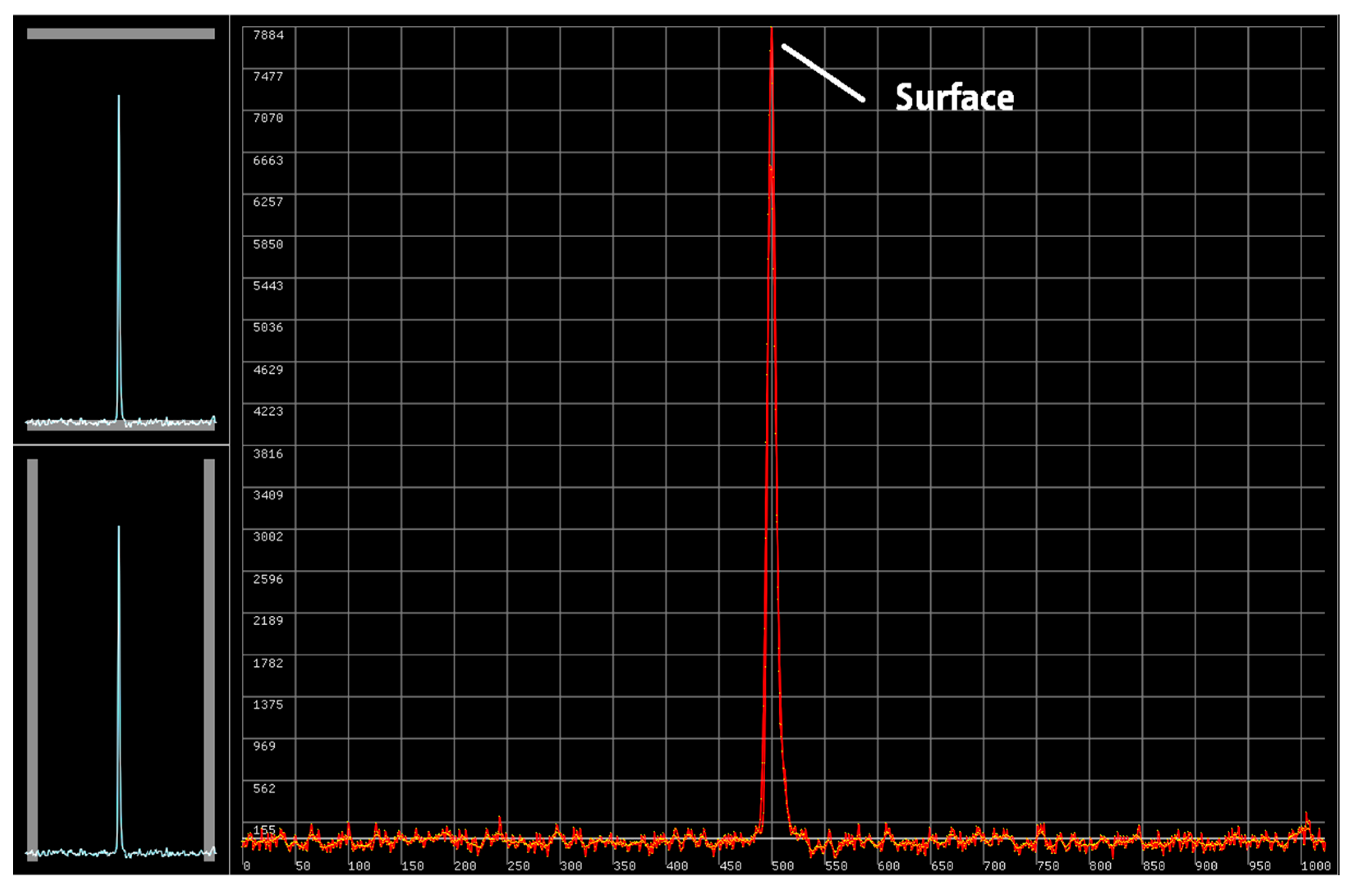
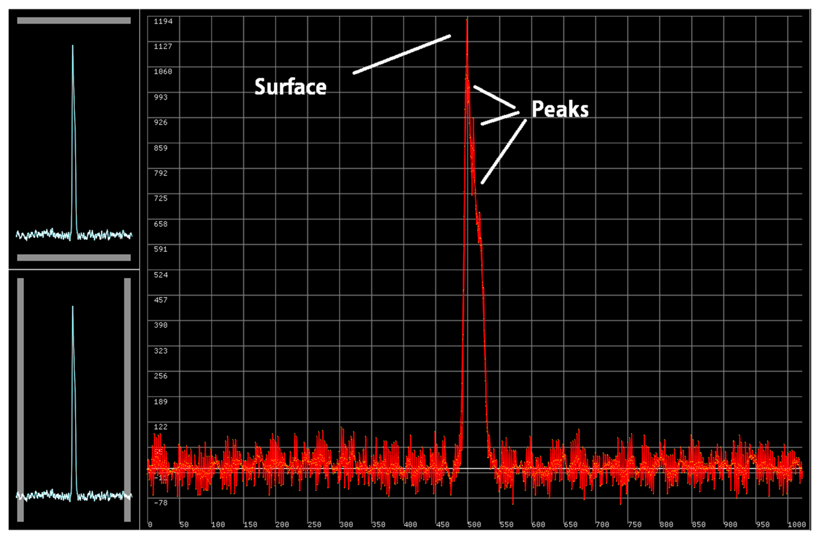
  • Class 0 returns represent the water surface synthetically and they are interpolated using a proprietary AHAB algorithm. The NIR channel measurements estimate the water surface’s elevation, and the algorithm uses the synthetic surface to inform the selection of peaks in the green channel waveform.
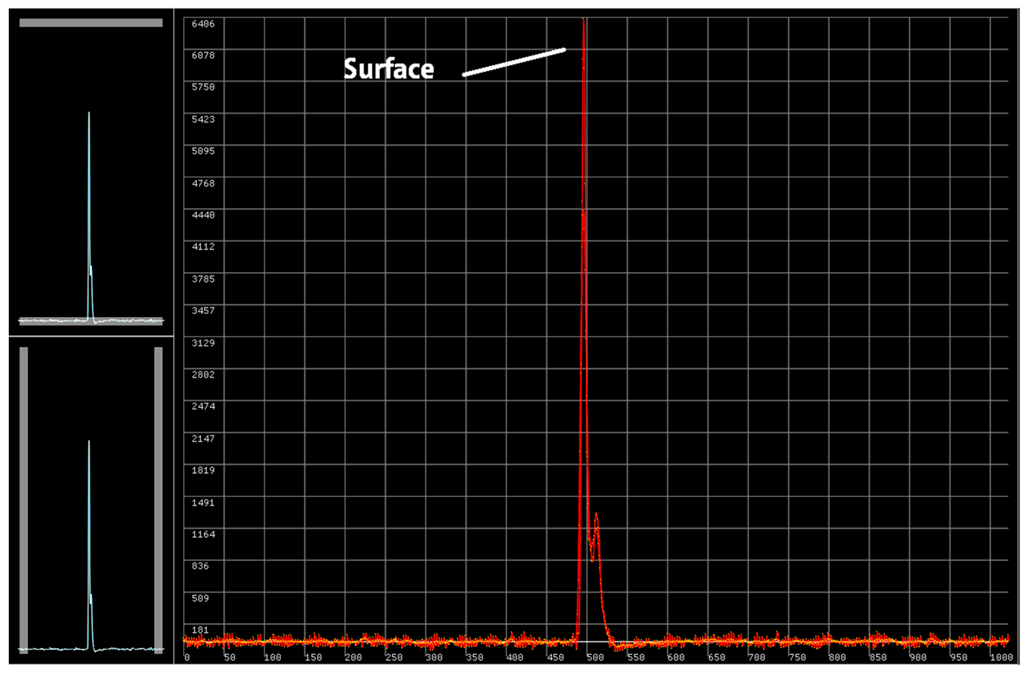
  • Class 5 returns represent the water surface and are calculated by picking out the first strong peak from the green channel waveform without using data from the NIR channel.
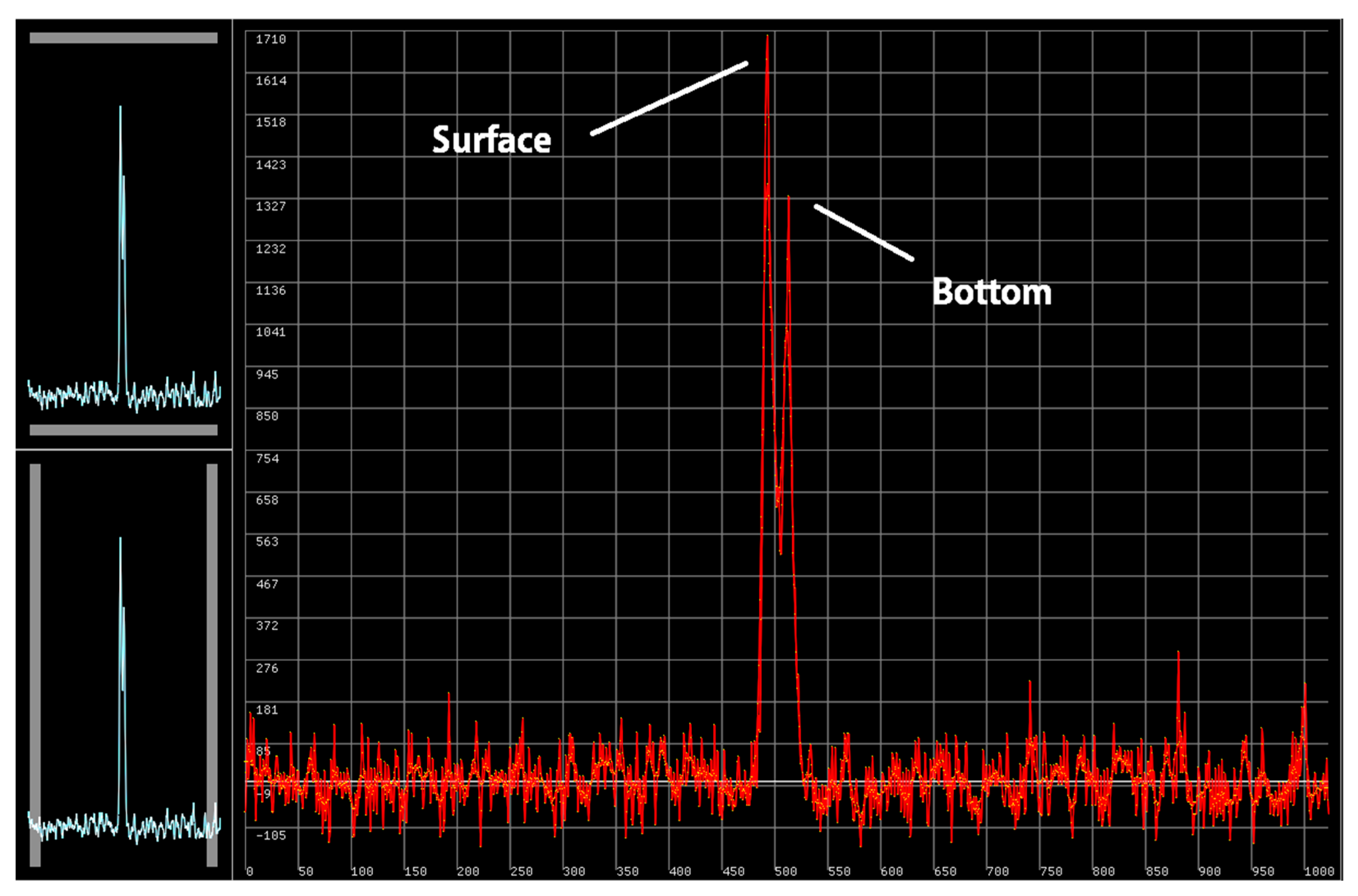
  • Class 7 returns represent a reflective surface in the water column and are calculated by selecting a second strong peak from the waveform.
  • Class 10 returns represent a reflective surface in the water column and are calculated using peaks of lower amplitude than those used in Class 7. The weaker peaks are selected using a proprietary algorithm to improve the lidar system’s depth-measuring capability by discarding peaks created by low or moderate turbidity levels.
In Equation (2), dm is the distance traveled in meters, n is the refractive index of the water, Cw is the speed of light in the water, and f is the digitizer sampling rate in gigahertz (GHz). The refractive index changes with water temperature (T), salinity (S, ‰), and the wavelength of the emitted beam (λ). To estimate the irregularity in refractive index value, we used a tool built into LLSS v2.4 that computes the surface representation using the refraction equation (Equation (3)) [25]. This equation determined each refraction coefficient (n0 to n9) using the least-squares method to match the terms as a function of wavelength, salinity, and temperature at a given atmospheric pressure [26]. We considered the water temperature as 25 °C (T), typical for May; therefore, S = 35‰, and n = 1.343.
d m = C w   t 2 n f
n S , T ,   λ = n 0 + n 1 + n 2 T + n 3 T 2 S + n 4 T 2 + n 5 + n 6 S + n 7 T λ + n 8 λ 2 + n 9 λ 3
It is possible to compute the duration of each sample (td) by dividing the time difference (Δt) by the system sampling rate (f) (Equation (4)). We can also calculate the vertical spacing between the lidar pulses traveling in space and the water column. Assuming the refraction is constant, such as in a vacuum (n = 1), each sample represents a spacing of 0.167 m. In seawater, with the addition of a higher refraction index and the slowing light propagation, the sample spacing decreases, e.g., n = 1.342, and the spacing equals 0.0931 m between the samples.
t d = 1 f × t
The accuracy of the lidar-derived measurements relies on the calibration of individual system components. The eccentricity and misalignment between the laser mirrors, the inertial movement unit (IMU), and the GPS antenna must be determined precisely. The process requires collecting height measurements of a relatively flat surface using a geodetic-grade GPS and comparing these heights to lidar measurements. For this purpose, we surveyed the Port Isabel-Cameron County airport (KPIL) taxiway using a Trimble R8 receiver. Static GPS survey points were post-processed to improve their positioning using a TxDOT (Texas Department of Transportation) maintained TXLN (Texas Laguna Madre, 26°5”41.6392′N, −97°18”02.4998′W) NOAA-CORS (National Oceanic and Atmospheric Administration-Continuously Operating Reference System) base station.

2.6. Satellite Imagery and Pixel Reflectance Analysis

Satellites with high-resolution imaging sensors can capture information on large areas, allowing identification of various features. Because Lower Laguna Madre is dynamic, and airborne lidar measurements were acquired in May and June, we downloaded imagery acquired solely in May and June 2016–2019 for temporal study purposes. We omitted 2020 imagery due to clouds blocking in-situ measurement locations.
The European Space Agency operates the Sentinel series satellites, and the Payload Data Ground Segment unit processes Level-1C (L1C) products and outputs radiometrically and geometrically corrected top-of-atmosphere images. L1C products are composed of 100 × 100 km tiles, including cloud masks and European Centre for Medium-Range Weather Forecasts information (total ozone column, water vapor, and MSL pressure). Every L1C product registers information with wavelength bands 1 to 9 (442 to 864 nm). Bands 2-blue, 3-green, 4-red, 5-red edge, and 8-NIR (492, 559, 664, 704, and 832 nm) were essential to this study because of their capability to distinguish the differences in pixel reflectance values, emphasizing the boundary between land and water [27]. The spatial resolution varied with each band: 10 m per pixel for bands 2 to 4 and 8 and 20 m for band 5. Table 2 summarizes the sensing time, date, tile numbering, and other specifics of the downloaded imagery.
Analysis of EM radiation recorded from underwater reflectance and optics may supply essential information about quality, depth, and other distinctive properties of water. Therefore, we studied optical information and used algorithms to estimate bathymetry [28]. The blue-green and NIR wavelengths can distinguish the varying concentrations of suspended particulate matter in the water [29,30]. Previous studies indicated that Band 4 (665 nm) can distinguish the chlorophyll-A absorption, and Band 5 (705 nm) relates to the vegetation monitoring and turbidity patterns in shallow lagoons [31,32].
The ENVI Spectral Profile Tool was used to analyze the radiance recorded at each pixel. Our objective was to distinguish the areas with high turbidity; nevertheless, the pixel radiance values helped us to identify the features surrounding the lagoon (e.g., vegetation and dunes). Areas with clouds have exceedingly high reflectance values, and we generated masks to exclude these areas from further analysis. To plot the results, we used ENVI’s Iterative Self Organizing Data Analysis (ISODATA) clustering algorithm, an unsupervised classification tool that iteratively clusters pixels to the nearest class [33]. The algorithm does not require a priori knowledge of the surfaces. Instead, it computes the mean radiance values by reclassifying the pixels until the difference between them is less than the threshold (e.g., 2%) or the maximum number of iterations, ten by default, is achieved. The process is similar to K-means clustering, which has advantages for fast converging datasets and a simple implementation process [34]. Further, we conducted a Normalized Difference Water Index [NDWI = (green − NIR)/(green + NIR)] analysis to build a surface map by mounting the areas of interest [35]. Typically, NDWI analysis can detect moisture changes in vegetation [36], and we used the algorithm to exclude cloudy and vegetated areas as identified by the ISODATA analysis. The band reflectance was normalized (0–1) using the ENVI Band Math tool because the scaling factor normalizes the images to reduce radiometric differences across non-surface effects [37].

2.7. Satellite-Derived Bathymetry

We studied the satellite-derived bathymetry that utilizes ocean optics and algorithms to estimate depths [29]. Water-leaving radiance is the backscatter upwelling after traversing the air/water interface and recording subsurface volumetric and bottom information. Previous studies developed the bottom albedo-independent bathymetric algorithm that accurately distinguishes bottom types such as sand, rock, and vegetation up to 15 m depth under ideal atmospheric and water conditions [38,39].
The Spectral Processing Exploitation and Analysis Resource (SPEAR) algorithm in the Relative Water Depth tool in ENVI v5.5 allows analysts to understand bathymetric properties using the blue, green, and NIR bands (2, 3, 4, and 8). In this study, in-situ measurements were required to generate absolute results; therefore, we input depth values into 06/2017 imagery, which included a combination of TCEQ station observations and sonar waypoints, all relative to MSL.

3. On-Site Analysis

We conducted preliminary data processing activities immediately after each airborne data acquisition mission. Decimated (e.g., 1/100) vector datasets were output to confirm lidar swath coverage and height measurements.
Previously, in the Colorado River study [40], where water was deeper (up to 12 m) and relatively transparent, we observed an increase in Chiroptera’s bathymetric capability by 0.8 m (9.2%) using the Class 10 algorithm. In Lower Laguna Madre, where water was shallower than 3.35 m, the on-site analysis revealed a 41.2% depth measuring increase using the same algorithm (Table 3). In contrast, our analysis indicated a reduced correlation between Classes 0 and 5 (water surface) with increasing turbidity (Table 4). Naturally, escalating turbidity scattered Class 5 pulses, generating a less consistent surface representation. Therefore, we used Class 0 returns to define the water surface that averaged heights derived from returns of both wavelengths.
Additionally, we analyzed the influence of turbidity on the bathymetric capability of Chiroptera by studying the in-situ observations (Appendix A). We converted the turbidity measurements to logarithmic values, and the findings indicated a linear relationship (R2 = 0.82) between the maximum measurable depth (theoretical, Dmax) and escalating turbidity at locations where the bottom was not visible to the observer (Figure 3).

4. Results

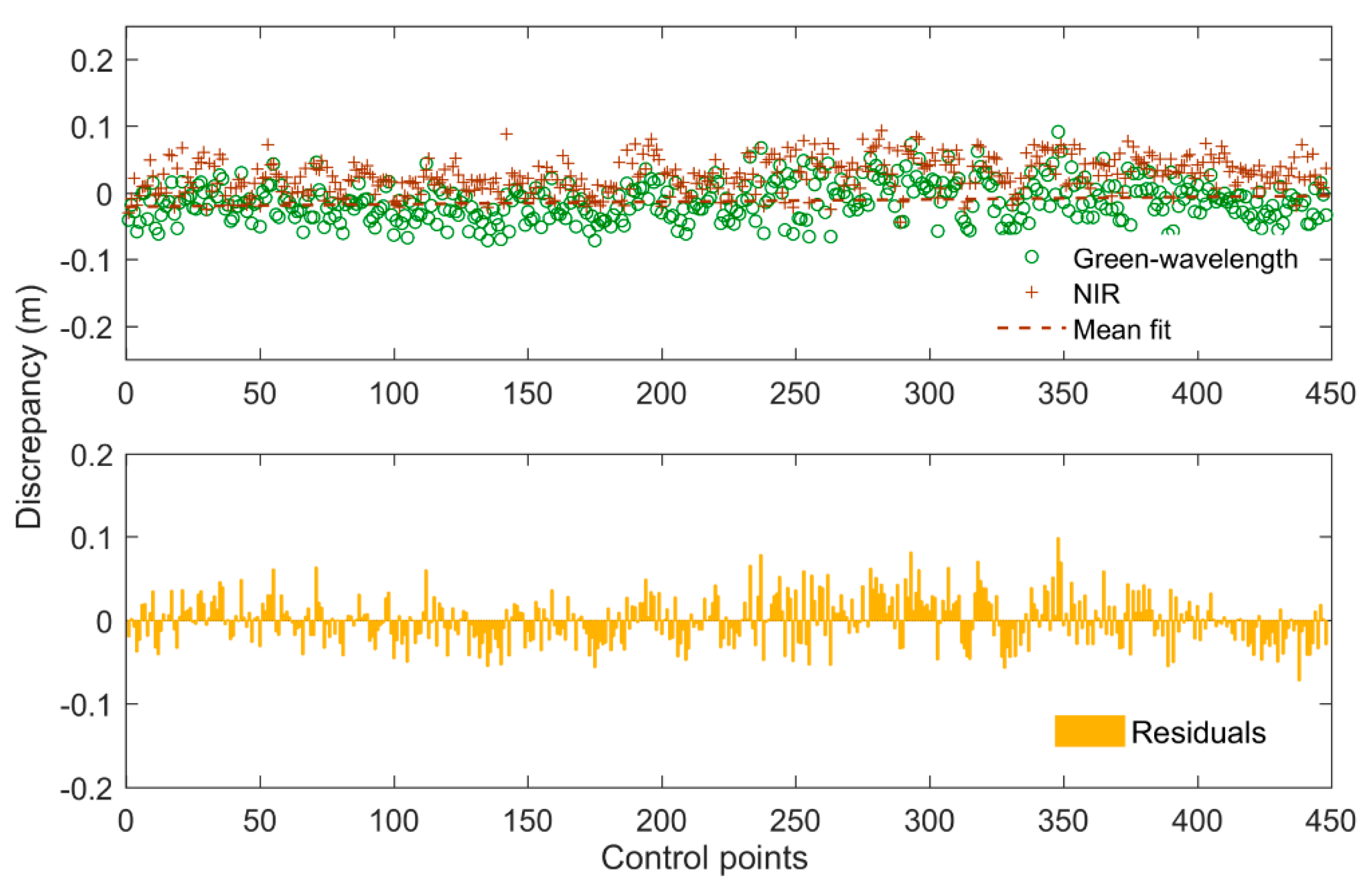
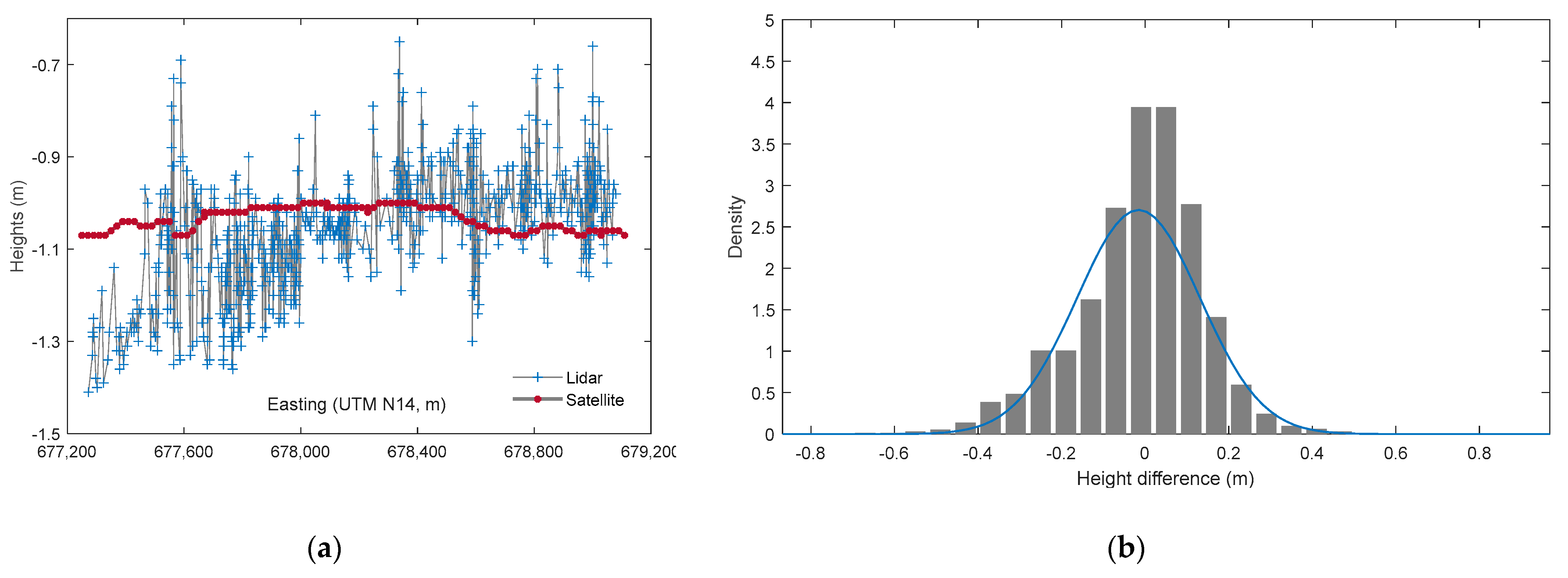
4.1. ALB System Calibration

Using the least-squares statistical method, we compared 448 ground GPS survey point elevations to lidar derived surface TIN patches [41]. For both scanners, the correlation produced high confidence (R2 > 0.95). Each scanner’s median height bias and RMSE were less than 2.8 cm. Findings revealed a minor height bias between the scanners (<4 cm), conceivably caused by NIR and green wavelength pulses registering different surface heights due to beam divergence differences (Table 5, Figure 4).

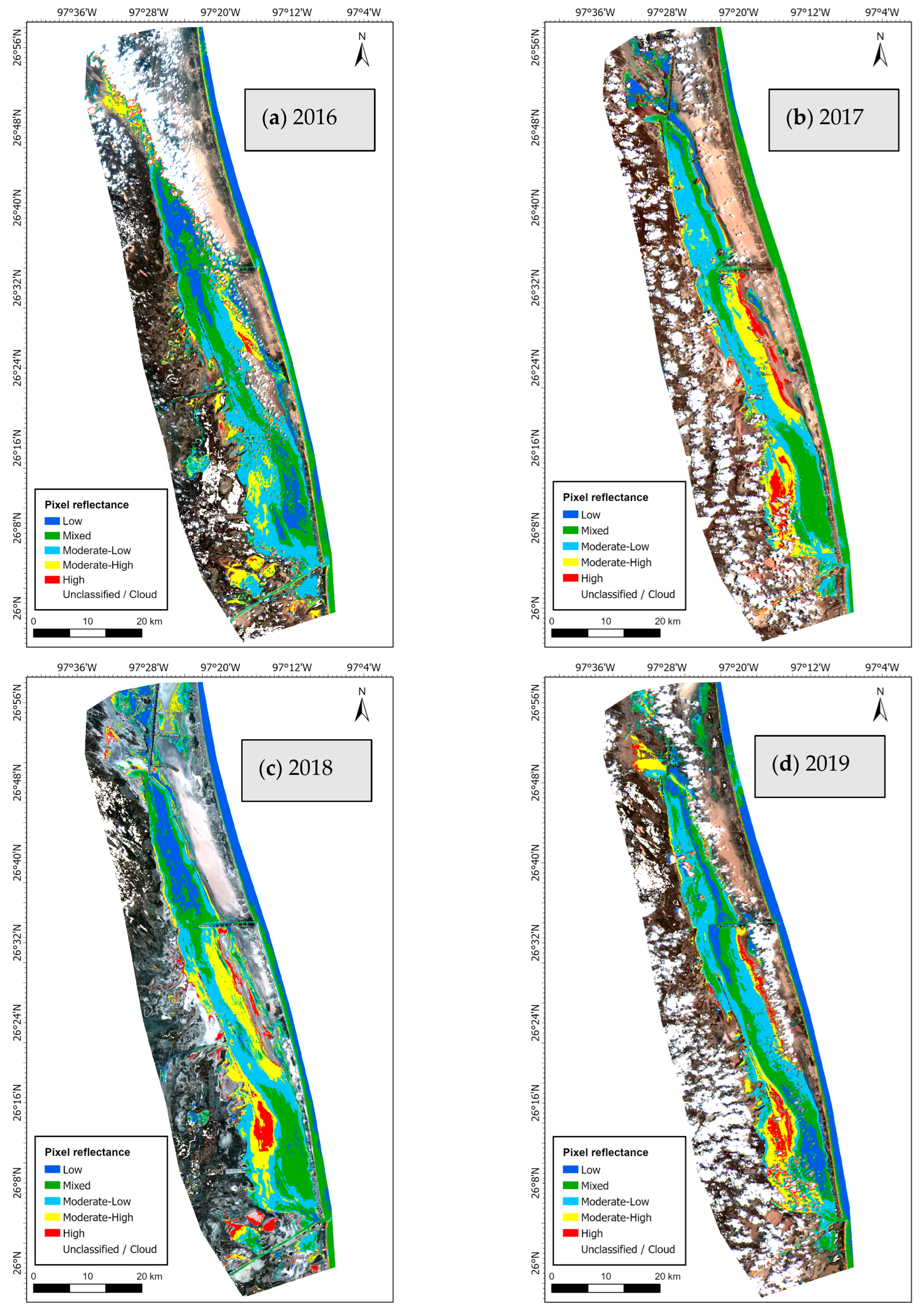
4.2. Pixel Reflectance

Six ISODATA classes of pixel reflectance (1-low, 2-mixed, 3-moderate-low, 4-moderate-high, 5-high, and 6-unclassified/cloud) were generated, which was in line with the Alaskan North Slope study [30]. The classifications were based on 2% spectral variability, and results omitted excessive turbid and unclassified/cloud areas using masking polygons. Table 6 presents the pixel count (%) of each image as the result of ISODATA classification, and the maps illustrate the dynamic nature of the lagoon by indicating the water quality variations (Figure 5a–d). Interpreting the results and predicting the temporal changes that occurred over the years is possible, and these variations can uncover potential geomorphological changes such as subsidence or coastal erosion. Additionally, results may highlight the need to update local charts and coastal geology maps.
We can assume the following statements by examining the findings:
  • In 2016, the average reflectance values were the lowest; therefore, the overall water quality was higher. Furthermore, the moderate-high and high reflectance classes indicated the lowest pixel counts (3.54%), confirming higher water quality, particularly in the southwestern parts of the lagoon (Figure 5a).
  • In 2017, the low reflectance classes were least significant (1.05%), while the mixed reflectance class registered (6.02%) as the most substantial, translating to the lowest water quality of all years analyzed (Figure 5b).
  • In 2018, pixel count was lower in moderate-high and high reflectance classes (5.22%), which translated to lower water quality. However, water quality has increased visibly in the northern parts of the lagoon (Figure 5c).
  • In 2019, the low reflectance class registered the highest pixel count (4.33%), resulting in the most suitable conditions for SDB analysis (Figure 5d).

4.3. Lidar Bathymetry

Chiroptera measured the lagoon bottom deepest at 3.35 m in Area-1 and 4.25 m on the northeastern edge of the survey area, at the Gulf coastline. Lidar measurements indicated the mean depth of the lagoon was no more than 0.61 m, where 42.65% of the depths registered were between 0.4 m and 1.2 m, and only 1.07% of measurements were deeper than 2 m (Figure 6).
We completed the lidar data acquisition campaign in approximately 60 flight hours. Due to the tides, surface datasets revealed height differences of 0.84 m (lowest = −0.28 m MSL, highest = 0.56 m MSL) in two weeks. The mean surface height was 0.04 m, and the standard deviation was 0.18 m throughout the data acquisition campaign. Surface height variation aligned with the 0.9 m tide range that was observed at the Port Isabel gauge in May 2017 (Figure 7).
We must emphasize that lagoon bottom measurements shallower than 0.4 m may not represent the true bottom due to the environmental limitations imposed by turbidity and the waveform sampling capability of Chiroptera’s digitizer. Particularly in moderately turbid sections of the lagoon, a considerable number of lidar beams penetrated the water column slightly. However, beams were scattered and reflected to the receiver by suspended material before reaching the bottom, causing very shallow depths or no depths to be registered. Therefore, measurements greater than 0.4 m (>51%) have a higher probability of being accurate and represent the actual lagoon bottom (Figure 8).

4.4. Lidar Bathymetry versus Sonar

The varying levels of turbidity and transparency influenced lidar and sonar measurements, especially in the southwestern and northern sections. A comparison of depths indicated that sonar (dS) recorded deeper versus lidar (dL) in all in-situ areas, and the mean difference was greater at locations with higher turbidity, which exposed a limitation of lidar bathymetry. Particularly in Area-3, where turbidity was the highest, lidar returns were scattered and attenuated rapidly, either on the immediate surface or in the water column, resulting in fewer matches between the measurements (Table 7). Investigating the results, we can consider the following statements for each of the in-situ areas:
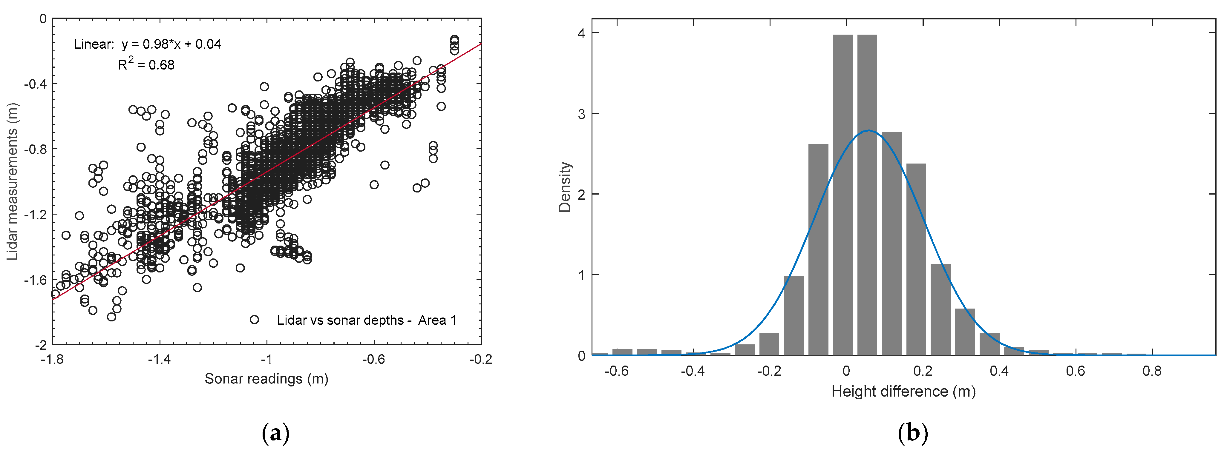
  • In Area-1, the water was shallow, the bottom was visible to the observer, and we sampled the lowest turbidity (2.7 NTU). Initially, the comparison algorithm returned poor correspondence efficiency (5%) in matching sonar to lidar measurements because of the sparse nature of sonar recordings. Therefore, we increased the distance of circumcenter triangle coverage (default dS1i = 1 m) of lidar TIN patches to 5 m and the height (h) tolerance to 1 m (default = 0.5 m). We kept the slope angle at the default setting (45°). As a result, the algorithm efficiency increased, and the matching rate improved (55%). The correspondence produced a linear relationship, where returns deeper than 1 m were scattered (R2 = 0.68). In this location, the average height for lidar/sonar was −0.87/−0.92 m MSL and the deepest measurement was −1.83 m MSL (Figure 9a,b).
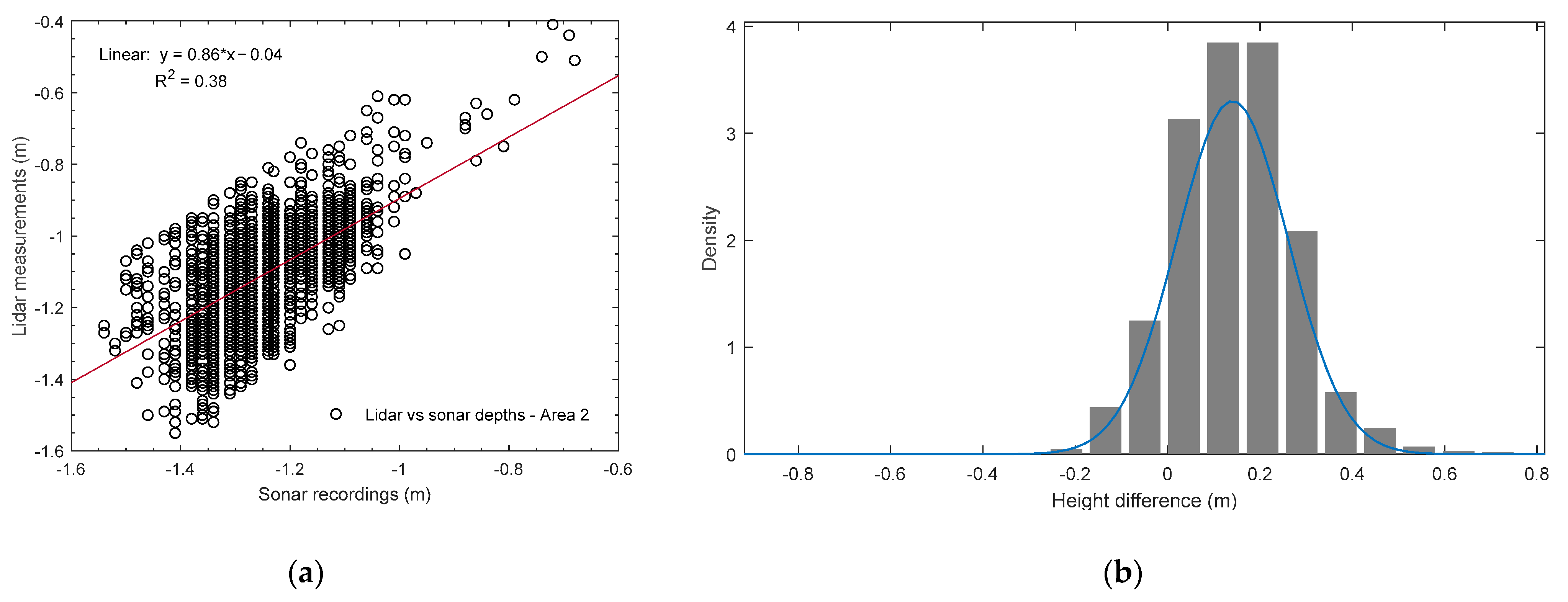
  • In Area-2, the lagoon bottom was partially visible, and we observed varying Secchi disk depths (0.6–0.9 m). Overall, turbidity has increased (8.6 NTU), and the comparison algorithm matched fewer sonar to lidar measurements (40%), producing less dependable matches, particularly in depths shallower than 1 m, indicating the increased turbidity. The mean lidar depth was −1.09 m MSL, and the sonar measured 14 cm deeper (−1.23 m MSL). The correspondence between the measurements was linear but produced a less favorable agreement (R2 = 0.38, Figure 10a,b).
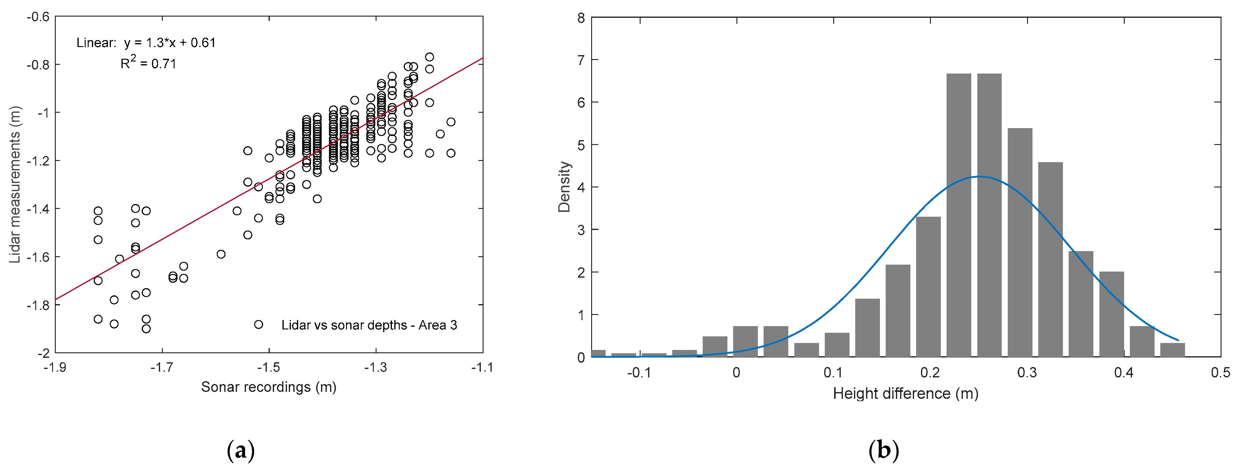
  • In Area-3, deeper bottom and poor water quality were observed. The Secchi disk depths were recorded between 0.7 and 1.3 m, and we sampled turbidity at 10.5 NTU; hence, lidar beam amplitudes were insufficient to measure the lagoon bottom. With default threshold parameters, the comparison algorithm produced unreliable results; consequently, we applied looser values to the experiment (dS1i = 10 m) and the algorithm included more legitimate matches. As a result, the matching efficiency dropped (8%), and generated a linear agreement (R2 = 0.71). The mean lidar depth was −1.14 m MSL, and sonar measured deeper at −1.39 m MSL (Figure 11a,b).

4.5. Satellite-Derived Bathymetry versus Lidar Bathymetry

We analyzed the 2017 Sentinel-2A imagery and investigated satellite-derived bathymetry of Lower Laguna Madre. The principal motivation was to compare and quantify the resultant satellite bathymetry to lidar measurements and study the compatibility, particularly in the in-situ areas. The satellite imagery’s varying turbidity, excessive shallow depths, and coarse grid spacing (20 m) were expected to adversely influence the bathymetric quality and completeness. Therefore, we assessed the comparison algorithm threshold values (e.g., dS1i = 5 m) and included more measurements in the computations. We must emphasize that satellite bathymetry was adjusted with local tides to match lidar measurements and observed MSL values were extracted from heights (depths).
We compared the SDB findings to lidar measurements at in-situ locations in Area-1 and Area-2 and omitted those in Area-3 because the location was blocked with excessive clouds. Because SDB measurements were coarse, the matching process did not produce a reliable correspondence. Using a 5 m threshold, in Area-1, where turbidity was lower, mean satellite bathymetry was 13 cm deeper compared to lidar measurements (−0.99 m versus −0.86 m MSL), and using a 10 m threshold, the mean difference was reduced to 11 cm. In Area-2, where turbidity and depths increased, we observed mean heights matching each other within 0.02 m (Table 8). To visualize the relationship further, we plotted sample height profiles and produced histograms (Figure 12 and Figure 13). In both in-situ locations, SDB produced linear measurements with a low standard deviation (0.03 m), where lidar measurements were scattered, and produced a higher standard deviation (0.16 m). We calculated the RMSE between the measurements at less than 0.15 m.
Studying the SDB results and their correspondence to lidar measurements at both in-situ locations, we can assume that the optical technology has depth-resolving limitations in shallow waters with varying turbidity. However, results suggested that SDB correlated adequately with lidar measurements, indicating the depth coarsely, and can be an effective method to evaluate the feasibility of conducting an expensive and comprehensive airborne lidar survey campaign.

5. Discussion

In this study, we acquired, processed, and analyzed remotely sensed datasets of Lower Laguna Madre and investigated the depths in the height domain. Our objective was driven by a desire to further understand and quantify the quality-control aspects of airborne lidar bathymetry with applicable survey methods, as we previously demonstrated at inland water reservoirs [14,15].
We summarized the best practices for airborne lidar data acquisition for the Frio River in Texas and mapped the river bottom. The study provided considerations for similar deployments where environmental conditions were almost ideal. At Devils River in southwestern Texas, the survey area included varied terrain with less favorable conditions, and submerged aquatic vegetation that blocked lidar and sonar measurements. Therefore, we used a variety of measurement methods and demonstrated the feasibility of merging airborne lidar measurements with GPS, sonar, and ground penetrating radar (GPR) recordings. The challenge was to align EM waves to each other, and we concluded the study by adjusting the propagation speed of GPR radio waves by measuring the water temperature and salinity.
In Laguna Madre, we conducted in-situ campaigns to understand the water properties and analyzed pixel reflectance to build spatial masks to distinguish land and water boundaries. Moreover, with reflectance maps, we were able to predict and classify areas that were impacted by turbidity. To align all measurements with each other, we converted lidar measurements to real world heights using the GEOID12B model, adjusted all measured depths to MSL, and applied applicable tide corrections, where applicable. The study demonstrated that in large and remote survey locations where in-situ measurements may not be practical or sufficient to cover all areas, satellite imaging pixel reflectance analysis can provide a cost-effective means of evaluating the feasibility of conducting airborne lidar surveys. Furthermore, lidar versus sonar depth comparison revealed adequate results that exceeded the Special-Order standards set by the International Hydrographic Organization (total vertical uncertainty < 0.26 m, depths shallower than 10 m, [42]).
Our study concludes that higher levels of turbidity (>2.7 NTU) reduced the correlation confidence between sonar and lidar measurements and adversely impacted the confidence in lidar measurements. We confirmed that lidar beams were not able to map 48% of the lagoon bottom due to environmental and technical limitations, demonstrating an important limitation of the technology. Nevertheless, airborne lidar bathymetry is detailed and accurate, particularly in shallow and relatively transparent waters. Concluding our study, we aimed to fill the gap in the literature with lidar mapping of water reservoirs that are subject to diverse environmental conditions and excessively shallow depths. We demonstrated that prior to airborne lidar data acquisition, researchers should investigate the local wind and tide patterns, account for aquatic vegetation growth season, and plan the airborne campaign accordingly.

6. Conclusions

In conclusion, we addressed doubts concerning the reliability of water bottom measurements using airborne lidar and optical imaging methods to support bathymetric mapping efforts in a hyper-saline lagoon in southern Texas. Overall, we conclude the following as the answers to our research questions outlined in the introduction:
  • Measuring the lagoon bottom with airborne lidar has practical and theoretical limitations. This advanced technology is expensive but effective and produces highly detailed vector data. Therefore, we suggest that researchers should carefully study local environmental conditions and modify survey areas before the data acquisition campaign.
  • In-situ campaigns are an essential practice of mapping with airborne lidar bathymetry. As demonstrated, we recommend careful planning and executing in-situ campaigns with airborne missions. Sonar surveys are invaluable to confirm the bottom (or depth) measurements attained by airborne lidar; however, sonar units require calibration to align with the survey location’s environmental conditions.
  • Our study highlights the need to conduct satellite imaging analysis before surveying estuaries and oceanic areas using an airborne lidar system applicable to large inland water reservoirs. Analysts can estimate and modify their survey requirements with the resultant pixel reflectance analysis and predict the areas with low water quality that may directly influence the remotely sensed bottom measurements.
  • Airborne lidar bathymetry is more detailed compared to SDB. Coarse grid sampling of satellite bathymetry limited a comprehensive depth comparison and cross-use of datasets. However, the study results indicated adequate agreement between the measurements, particularly in the relatively transparent sections of the lagoon.
In Lower Laguna Madre, the water conditions were variable, and depths were shallow for effective airborne lidar mapping efforts. Our study indicated that 51% of the lagoon was in acceptable limits of bathymetric mapping (deeper > 0.4 m). However, we should emphasize that even in transparent water conditions, shallower depths would push the theoretical and practical bottom mapping limitations of the technology. It is common that an ALB can map depths exceeding 40 m, and SDB is effective up to 20 m in ideal environmental conditions, and both technologies have proven their effectiveness. However, we intended to fill the gap in the literature that these technologies are not novel, but they have theoretical and practical limitations, particularly in dynamic estuaries and oceanic environments.

Author Contributions

K.S. served as the principal investigator, conducted data processing and analysis, and drafted the article. A.B. analyzed satellite imagery and contributed to the relevant sections of the article. J.R.A. modified lidar datasets and generated raster maps and contributed to the article. A.R.A. operated the airborne lidar instrument and contributed to the data analysis. All authors have read and agreed to the published version of the manuscript.

Funding

The Texas General Land Office (GLO) funded the Data acquisition campaign (2017, contract no. 16-201-000), and Jeffrey Paine served as the principal investigator. The Texas Water Development Board (TWDB) funded the data analysis project (2021, contract no. 2101792506) and Kutalmis Saylam served as the principal investigator.

Data Availability Statement

The data presented in this study are available on request from the corresponding author. The data are not publicly available due to size and limited storage availability.

Acknowledgments

TWDB staff Caimee Schoenbaechler, Amin Kiaghadi, and Joey Thomas supplied valuable feedback. Aspen Helicopters of Oxnard, California, provided the survey aircraft and the aircrew. BEG researchers Tiffany Caudle and John Hupp participated in fieldwork and contributed to field data processing. Jackson School of Geosciences graduate student Shelby Short assisted with the article graphics. University of Ottawa faculty Anders Knudby provided valuable feedback. We thank all others who were involved and made this comprehensive study possible.

Conflicts of Interest

The authors declare no conflict of interest.

Abbreviations

UTM EUniversal Transverse Mercator–Easting (m)
UTM NUniversal Transverse Mercator–Northing (m)
Avg. NTUAverage measured turbidity in nephelometric turbidity unit
SecchiObserved Secchi disk depth (m)
KdDiffuse attenuation coefficient
VBWater bottom is visible to the observer
WPWaypoint location marked for a sonar measurement (observer-triggered measurement)
Avg. sonar depthAverage depth of all sonar measurements in a 1 m radius (automatically derived)
CL0Lidar vector data, Class 0, surface, NIR + green wavelength
CL7Lidar vector data, Class 7, bottom, green wavelength, standard bathymetric algorithm
CL10Lidar vector data, Class 10, bottom, green wavelength, enhanced bathymetric algorithm
N/ANot Applicable

Appendix A

Table A1. Turbidity and Sonar Depth Measurements.
LocationSurvey AreaDateUTM EUTM NReading 1Reading 2Reading 3AVG NTUSecchi (m)KdWP SNR Depth (m)Avg. SNR Depth (m)Lidar Depth CL0–CL7 (m)Lidar Depth CL0–CL10 (m)
212017-05-01681,989.952,891,306.110.600.700.610.64VBN/A1.491.131.06N/A
32017-05-01682,546.592,891,234.732.212.492.812.50VBN/A1.851.831.082.16
42017-05-01681,723.882,891,259.922.102.022.012.04VBN/A1.261.291.341.53
52017-05-01680,939.152,891,230.512.382.992.792.72VBN/A1.381.381.421.50
62017-05-01681,101.492,890,944.681.601.811.991.80VBN/A1.351.381.401.47
72017-05-01681,434.532,890,731.421.902.162.242.10VBN/A1.381.301.231.41
82017-05-01681,985.002,890,432.002.823.704.553.69VBN/A1.331.331.371.47
92017-05-01682,282.752,890,039.692.813.183.263.08VBN/AN/A1.271.341.59
102017-05-01681,075.642,889,328.481.751.521.991.75VBN/A1.191.221.111.40
112017-05-01680,624.582,888,914.093.363.624.103.69VBN/A1.281.330.05N/A
122017-05-01680,311.532,889,005.784.645.265.685.19VBN/A1.451.441.441.63
1322017-05-05678,831.782,894,403.481.311.511.591.47VBN/A1.281.251.37N/A
142017-05-05678,364.022,894,849.481.341.821.811.66VBN/A1.191.211.351.38
152017-05-05677,943.082,895,043.142.792.933.393.04VBN/A1.231.231.13N/A
162017-05-05677,471.312,895,420.793.667.908.026.53VBN/A1.401.401.491.63
172017-05-05677,293.562,895,990.833.7811.5012.209.16VBN/A1.261.42N/A1.85
182017-05-05676,829.282,896,189.4715.9017.3019.3017.500.62.671.611.63N/A2.17
192017-05-05677,032.682,897,036.1710.2015.5016.4014.030.72.291.521.53N/A1.97
202017-05-05677,611.282,897,369.097.579.0411.009.200.851.881.381.351.541.22
212017-05-05677,341.542,898,209.334.274.955.524.91VBN/A1.451.411.671.72
222017-05-05676,915.172,897,588.568.6911.5012.3010.830.72.291.571.541.271.59
232017-05-05677,020.092,896,493.0810.5012.8012.7012.000.91.781.571.57N/A2.58
242017-05-05676,501.322,895,309.6914.0018.9019.7017.530.82.001.661.67N/AN/A
252017-05-05677,336.302,894,813.243.853.433.903.73VBN/A1.421.421.511.73
2632017-05-12672,597.732,888,097.9211.1015.7016.7014.500.72.291.831.79N/A1.96
272017-05-12673,745.522,887,921.1411.1017.1021.7016.630.72.291.971.97N/A2.04
282017-05-12674,964.062,887,817.439.4813.5016.1013.030.72.291.901.90N/AN/A
292017-05-12676,179.752,887,926.158.9111.9012.1010.970.851.882.132.15N/AN/A
302017-05-12676,968.382,888,786.303.124.005.054.061.31.231.521.511.251.45
312017-05-12675,270.362,888,720.859.0315.8019.0014.610.72.291.921.94N/AN/A
322017-05-12674,052.802,888,881.7910.8013.4013.2012.470.82.002.022.01N/A1.86
332017-05-12674,961.022,889,283.6115.2015.0016.5015.570.752.132.062.02N/AN/A
342017-05-12676,290.012,889,264.615.448.229.337.6611.601.901.89N/A2.61
352017-05-12676,841.892,889,261.021.802.803.092.56VBN/A1.591.551.331.51
362017-05-12677,419.182,889,228.252.473.334.083.29VBN/A1.591.541.331.48

Appendix B. Lidar Bathymetry Waveform Classes

Figure A1. Class 0. Synthetic water surface is interpolated using a proprietary algorithm. A strong NIR backscatter surface peak estimates the elevation of the water surface, confirmed by the immediate peaks in the green wavelength.
Remotesensing 15 05754 g0a1
Figure A2. Class 5. Water surface represented by the first strong backscatter peak from the green wavelength waveform, without the use of an NIR channel.
Remotesensing 15 05754 g0a2
Figure A3. Class 7. Last return originating from a reflective backscatter surface (or the bottom) in the water column and calculated by a strong peak in the waveform.
Remotesensing 15 05754 g0a3
Figure A4. Class 10. A reflective surface (or bottom) detected in the water column and calculated using peaks of lower amplitude than those used in Class 7.
Remotesensing 15 05754 g0a4

References

  1. Höfle, B.; Rutzinger, M. Topographic Airborne LiDAR in Geomorphology: A Technological Perspective. Z. Für Geomorphol. 2011, 55, 1–29. [Google Scholar] [CrossRef]
  2. Lohani, B.; Ghosh, S. Airborne LiDAR Technology: A Review of Data Collection and Processing Systems. Proc. Natl. Acad. Sci. India Sect. A Phys. Sci. 2017, 87, 567–579. [Google Scholar] [CrossRef]
  3. Guenther, G.C. Airborne Lidar Bathymetry. In Digital Elevation Model Technologies and Applications: The DEM User’s Manual; American Society of Photogrammetry and Remote Sensing, Pennsylvania State University Press: University Park, PA, USA, 2007; pp. 253–320. [Google Scholar]
  4. Mandlburger, G. Bathymetry from Images, LiDAR, and Sonar: From Theory to Practice. PFG–J. Photogramm. Remote Sens. Geoinf. Sci. 2021, 89, 69–70. [Google Scholar] [CrossRef]
  5. Brock, J.C.; Purkis, S.J. The Emerging Role of Lidar Remote Sensing in Coastal Research and Resource Management. J. Coast. Res. 2009, 10053, 1–5. [Google Scholar] [CrossRef]
  6. Klemas, V. Beach Profiling and Lidar Bathymetry: An Overview with Case Studies. J. Coast. Res. 2011, 277, 1019–1028. [Google Scholar] [CrossRef]
  7. Paine, J.G.; Caudle, T.L.; Andrews, J.R. Shoreline and Sand Storage Dynamics from Annual Airborne LIDAR Surveys, Texas Gulf Coast. J. Coast. Res. 2017, 333, 487–506. [Google Scholar] [CrossRef]
  8. Toure, S.; Diop, O.; Kpalma, K.; Maiga, A. Shoreline Detection Using Optical Remote Sensing: A Review. ISPRS Int. J. Geo-Inf. 2019, 8, 75. [Google Scholar] [CrossRef]
  9. Dogliotti, A.I.; Ruddick, K.G.; Nechad, B.; Doxaran, D.; Knaeps, E. A Single Algorithm to Retrieve Turbidity from Remotely Sensed Data in All Coastal and Estuarine Waters. Remote Sens. Environ. 2015, 156, 157–168. [Google Scholar] [CrossRef]
  10. Garg, V.; Senthil Kumar, A.; Aggarwal, S.P.; Kumar, V.; Dhote, P.R.; Thakur, P.K.; Nikam, B.R.; Sambare, R.S.; Siddiqui, A.; Muduli, P.R.; et al. Spectral Similarity Approach for Mapping Turbidity of an Inland Waterbody. J. Hydrol. 2017, 550, 527–537. [Google Scholar] [CrossRef]
  11. Caballero, I.; Stumpf, R.P. Retrieval of Nearshore Bathymetry from Sentinel-2A and 2B Satellites in South Florida Coastal Waters. Estuar. Coast. Shelf Sci. 2019, 226, 106277. [Google Scholar] [CrossRef]
  12. Ji, X.; Yang, B.; Tang, Q.; Xu, W.; Li, J. Feature Fusion-Based Registration of Satellite Images to Airborne LiDAR Bathymetry in Island Area. Int. J. Appl. Earth Obs. Geoinf. 2022, 109, 102778. [Google Scholar] [CrossRef]
  13. Yeu, Y.; Yee, J.-J.; Yun, H.; Kim, K. Evaluation of the Accuracy of Bathymetry on the Nearshore Coastlines of Western Korea from Satellite Altimetry, Multi-Beam, and Airborne Bathymetric LiDAR. Sensors 2018, 18, 2926. [Google Scholar] [CrossRef]
  14. Saylam, K.; Hupp, J.; Andrews, J.; Averett, A.; Knudby, A. Quantifying Airborne Lidar Bathymetry Quality-Control Measures: A Case Study in Frio River, Texas. Sensors 2018, 18, 4153. [Google Scholar] [CrossRef] [PubMed]
  15. Saylam, K.R.; Averett, A.; Costard, L.; D. Wolaver, B.; Robertson, S. Multi-Sensor Approach to Improve Bathymetric Lidar Mapping of Semi-Arid Groundwater-Dependent Streams: Devils River, Texas. Remote Sens. 2020, 12, 2491. [Google Scholar] [CrossRef]
  16. McManus, J. Hydrodynamics of Estuaries Edited by Bjorn Kjerfve, Vol II Estuarine Case Studies, CRC Press, 1988. No. of Pages: 125. Earth Surf. Process. Landf. 1990, 15, 384–385. [Google Scholar] [CrossRef]
  17. Tunnell, J.W.; Judd, F.W. (Eds.) The Laguna Madre of Texas and Tamaulipas, 1st ed.; Gulf Coast studies; Texas A&M University Press: College Station, TX, USA, 2002; ISBN 978-1-58544-133-4. [Google Scholar]
  18. Dubin, J.T.; Ballard, M.S.; Lee, K.M.; McNeese, A.R.; Sagers, J.D.; Venegas, G.R.; Rahman, A.F.; Wilson, P.S. Compressional and Shear in Situ Measurements in the Lower Laguna Madre. J. Acoust. Soc. Am. 2018, 143, 1712. [Google Scholar] [CrossRef]
  19. Webster, T.; McGuigan, K.; Crowell, N.; Collins, K.; McDonald, C. Acquisition and Processing of Topo-Bathymetric Lidar for Isle Madame in Support of the World Class Tanker Safety Initiative; NSCC Applied Geomatics Research Group: Middleton, NS, USA, 2015; pp. 1–56. [Google Scholar]
  20. Kinzel, P.J.; Wright, C.W.; Nelson, J.M.; Burman, A.R. Evaluation of an Experimental LiDAR for Surveying a Shallow, Braided, Sand-Bedded River. J. Hydraul. Eng. 2007, 133, 838–842. [Google Scholar] [CrossRef]
  21. Estrada, J. Investigating the Effects of Nutrient Limitation, Light, and Salinity upon Seagrass Cover in the Lower Laguna Madre; GIS in Water Resources; The University of Texas at Austin: Austin, TX, USA, 2018; p. 11. [Google Scholar]
  22. Medwin, H. Speed of Sound in Water: A Simple Equation for Realistic Parameters. J. Acoust. Soc. Am. 1975, 58, 1318–1319. [Google Scholar] [CrossRef]
  23. Habib, A. Accuracy, Quality Assurance and Quality Control of Lidar Data. In Topographic Laser Ranging and Scanning: Principles and Processing; Taylor & Francis: Boca Raton, FL, USA, 2009; pp. 269–294. ISBN 978-1-4200-5142-1. [Google Scholar]
  24. Boris, Delaunay, Sur la sphere vide. Izv. Akad. Nauk SSSR Otdelenie Matematicheskii i Estestvennyka Nauk 1934, 7, 793–800.
  25. Quan, X.; Fry, E.S. Empirical Equation for the Index of Refraction of Sea Water. Appl. Opt. 1995, 34, 3477. [Google Scholar] [CrossRef]
  26. Roswell, A.; Halikas, G. The Index of Refraction of Seawater; University of California San Diego, Scripps Institution of Oceanography: La Jolla, CA, USA, 1976; p. 121. [Google Scholar]
  27. Mondejar, J.P.; Tongco, A.F. Estimating Topsoil Texture Fractions by Digital Soil Mapping—A Response to the Long-Outdated Soil Map in the Philippines. Sustain. Environ. Res. 2019, 29, 31. [Google Scholar] [CrossRef]
  28. Ashphaq, M.; Srivastava, P.K.; Mitra, D. Review of Near-Shore Satellite Derived Bathymetry: Classification and Account of Five Decades of Coastal Bathymetry Research. J. Ocean Eng. Sci. 2021, 6, 340–359. [Google Scholar] [CrossRef]
  29. Saylam, K.; Brown, R.A.; Hupp, J.R. Assessment of Depth and Turbidity with Airborne Lidar Bathymetry and Multiband Satellite Imagery in Shallow Water Bodies of the Alaskan North Slope. Int. J. Appl. Earth Obs. Geoinf. 2017, 58, 191–200. [Google Scholar] [CrossRef]
  30. Gernez, P.; Lafon, V.; Lerouxel, A.; Curti, C.; Lubac, B.; Cerisier, S.; Barillé, L. Toward Sentinel-2 High Resolution Remote Sensing of Suspended Particulate Matter in Very Turbid Waters: SPOT4 (Take5) Experiment in the Loire and Gironde Estuaries. Remote Sens. 2015, 7, 9507–9528. [Google Scholar] [CrossRef]
  31. Delegido, J.; Verrelst, J.; Alonso, L.; Moreno, J. Evaluation of Sentinel-2 Red-Edge Bands for Empirical Estimation of Green LAI and Chlorophyll Content. Sensors 2011, 11, 7063–7081. [Google Scholar] [CrossRef] [PubMed]
  32. Sebastiá-Frasquet, M.-T.; Aguilar-Maldonado, J.A.; Santamaría-Del-Ángel, E.; Estornell, J. Sentinel 2 Analysis of Turbidity Patterns in a Coastal Lagoon. Remote Sens. 2019, 11, 2926. [Google Scholar] [CrossRef]
  33. Ahmad, A.; Sufahani, S.F. Analysis of Landsat 5 TM Data of Malaysian Land Covers Using ISODATA Clustering Technique. In Proceedings of the 2012 IEEE Asia-Pacific Conference on Applied Electromagnetics (APACE), Melaka, Malaysia, 11–13 December 2012; IEEE: Melaka, Malaysia, 2012; pp. 92–97. [Google Scholar]
  34. Yuan, C.; Yang, H. Research on K-Value Selection Method of K-Means Clustering Algorithm. Multidiscip. Sci. J. 2019, 2, 226–235. [Google Scholar] [CrossRef]
  35. Wang, X.; Ling, F.; Yao, H.; Liu, Y.; Xu, S. Unsupervised Sub-Pixel Water Body Mapping with Sentinel-3 OLCI Image. Remote Sens. 2019, 11, 327. [Google Scholar] [CrossRef]
  36. Kaplan, G.; Avdan, U. Object-Based Water Body Extraction Model Using Sentinel-2 Satellite Imagery. Eur. J. Remote Sens. 2017, 50, 137–143. [Google Scholar] [CrossRef]
  37. de Carvalho, O.; Guimarães, R.; Silva, N.; Gillespie, A.; Gomes, R.; Silva, C.; de Carvalho, A. Radiometric Normalization of Temporal Images Combining Automatic Detection of Pseudo-Invariant Features from the Distance and Similarity Spectral Measures, Density Scatterplot Analysis, and Robust Regression. Remote Sens. 2013, 5, 2763–2794. [Google Scholar] [CrossRef]
  38. Favoretto, F.; Morel, Y.; Waddington, A.; Lopez-Calderon, J.; Cadena-Roa, M.; Blanco-Jarvio, A. Testing of the 4SM Method in the Gulf of California Suggests Field Data Are Not Needed to Derive Satellite Bathymetry. Sensors 2017, 17, 2248. [Google Scholar] [CrossRef] [PubMed]
  39. Stumpf, R.P.; Holderied, K.; Sinclair, M. Determination of Water Depth with High-Resolution Satellite Imagery over Variable Bottom Types. Limnol. Oceanogr. 2003, 48, 547–556. [Google Scholar] [CrossRef]
  40. Saylam, K.; Hupp, J.R.; Aaron, R.A. Quantifying the Bathymetry of the Lower Colorado River Basin, Arizona, with Airborne Lidar; researchgate: Baltimore, MD, USA, 2017; Volume 1, pp. 1–11. [Google Scholar]
  41. Savitzky, A.; Golay, M.J.E. Smoothing and Differentiation of Data by Simplified Least Squares Procedures. Anal. Chem. 1964, 36, 1627–1639. [Google Scholar] [CrossRef]
  42. IHO. International Hydrographic Organization, Standards for Hydrographic Surveys; International Hydrographic Bureau: Monaco City, Monaco, 2020; pp. 1–51. [Google Scholar]
Figure 1. (a) Aerial image of Area-1. The turbidity was low, the lagoon was shallow, and the bottom was visible for observations. (b) Aerial image of Area-3. Turbidity and floating vegetation created challenges for bottom measuring.
Remotesensing 15 05754 g001
Figure 2. Lower Laguna Madre in southern Texas and in-situ locations (TCEQ reference stations, NOAA tide gauges, and BEG observation areas). The yellow polygon indicates the extent of the airborne survey area (1600 km2).
Remotesensing 15 05754 g002
Figure 3. The influence of increasing turbidity on the theoretical bathymetric capability (maximum depth: Dmax) of Chiroptera is a linear relationship (R2 = 0.82).
Remotesensing 15 05754 g003
Figure 4. Comparison of heights as measured by each Chiroptera scanner. Results indicated a median bias of less than 4 cm measured from an altitude of 500 m.
Remotesensing 15 05754 g004
Figure 5. (ad) Pixel reflectance as recorded with Sentinel-2A L1C Band 5, classified using ENVI v5.5 ISODATA algorithm.
Remotesensing 15 05754 g005
Figure 6. Lidar bathymetry of the entire lagoon. The mean depth was 0.61 m, and 42.65% of all measurements were between 0.4 and 1.2 m.
Remotesensing 15 05754 g006
Figure 7. Surface elevation variation during airborne data acquisition campaign. The mean height was 0.04 m, and the standard deviation was 0.18 m.
Remotesensing 15 05754 g007
Figure 8. Lagoon bottom as measured with Chiroptera. 51% percent of the lagoon depths were greater than 0.4 m.
Remotesensing 15 05754 g008
Figure 9. (a,b). In Area-1, lidar and sonar heights produced a linear agreement (R2 = 0.68), indicating higher turbidity levels in depths greater than 1 m. The sonar-recorded slightly deeper compared to lidar measurements (mean difference = 5 cm).
Remotesensing 15 05754 g009
Figure 10. (a,b). In Area-2, turbidity was high in depths shallower than 1 m (mean = 8.6 NTU), scattering and attenuating lidar pulses, influencing the correspondence between lidar and sonar measurements adversely (R2 = 0.38). The mean height difference was 14 cm.
Remotesensing 15 05754 g010
Figure 11. (a,b): In Area-3, turbidity was the highest (mean = 10.5 NTU) and increased with depth. Fewer sonar and lidar measurements were matched (8%) because of loose algorithm thresholds. The mean height difference increased to 25 cm, improving the regression, and generating a bi-modal distribution (R2 = 0.71).
Remotesensing 15 05754 g011
Figure 12. (a,b). SDB versus lidar bathymetry in 2017 in Area-1. Measurement differences produced a skewed distribution and SDB measured deeper than lidar (mean difference < 13 cm).
Remotesensing 15 05754 g012
Figure 13. (a,b). SDB versus lidar depths in 2017 in Area-2. Turbidity increased, and the confidence between the measurements declined (<61%), particularly in areas deeper than 1 m.
Remotesensing 15 05754 g013
Table 1. Chiroptera system settings in the Lower Laguna Madre survey.
ItemNIR (1064 nm) Green (515 nm)
Pulse repetition rate (PRF)100–300 kHz 36 kHz
Average lidar point density10 points/m2 (+side overlap)2 points/m2 (+side overlap)
Average flight altitude 400–600 m
Swath width and overlap rate250–300 m/30% overlap
Average aircraft survey speed110–130 knots
Table 2. Details of Sentinel-2A L1C imagery used in the study.
DateSensing Time
(UTC)
TileSun Elevation (Degrees)Sun Azimuth (Degrees)Cloud Coverage (%)
12/05/201617:11:44T14RPQ72113.620
12/05/201617:11:44T14RPP72.3111.124
16/06/201717:15:05T14RPQ72.996.96
16/06/201717:15:05T14RPP73946
17/05/201817:10:16T14RPQ72.4110.50
17/05/201817:10:16T14RPP72.8107.90
27/05/201917:16:29T14RPQ73.1104.525
27/05/201917:16:43T14RPP73.3101.616
Table 3. Bathymetric class data output (Classes 7 and 10) comparison to sonar recordings at BEG-observed in-situ locations.
In-Situ AreaNumber of Measurements
(Class 7/10)
Mean Sonar Depth
(m, MSL)
Mean Lidar Depth (m, MSL)
(Class 7/10)
(Class 7/10)
Standard Deviation (m)
(Class 7/10)
Bathymetric Improvement
(%)
1256/130−1.35−1.28/−1.570.14/0.2323
2381/140 −1.43−1.42/−1.780.17/0.3820.2
3551/272−1.84−1.35/−1.840.62/0.6341.2
Table 4. Turbidity and surface class data output (Classes 0 and 5) comparison. Escalating turbidity levels scattered Class 5 returns and adversely influenced root-mean-square error (RMSE) values.
In-Situ
Area
Mean Turbidity
(NTU)
Number of Returns
(Class 0/5)
Median Difference (m)
(Class 0 to 5)
RMSE (m)
(Class 0 to 5)
R2
12.7528/173−0.070.030.94
28.6907/653−0.090.060.65
310.5806/420−0.110.080.32
Table 5. Chiroptera ALB system height calibration results.
Scanner Number of SamplesData Range (m)Median (m)RMSE (m)R2
NIR (1064 nm)4480.140.0250.0250.96
Green (515 nm) 4480.17−0.0130.0280.95
Table 6. Pixel reflectance count (%) of Lower Laguna Madre imagery, classified by ENVI’s ISODATA algorithm. N/A indicates the areas outside the study area.
ImageryPixel Reflectance Count (%)
1-Low2-Mixed3-Moderate-Low4-Moderate-High5-High6-Unclassified/CloudN/A
20164.165.796.112.970.580.0980.31
20171.056.025.583.181.050.0483.07
20183.945.685.514.081.140.1479.50
20194.334.915.372.661.180.0981.47
Table 7. Sonar versus lidar bathymetry comparison at in-situ locations.
In-Situ AreaMean Turbidity
(NTU)
Comparison Parameters (dSli, h, Slope Angle)Matching (%)Mean Depth (dL/dS, m, MSL)Difference (dL–dS, m)RMSE (m)R2
12.75/1/4555−0.87/−0.92−0.050.140.68
28.65/1/4540−1.09/−1.23−0.140.100.38
310.510/1/458−1.14/−1.39−0.250.090.71
Table 8. Comparison of SDB to lidar measurements in 2017. Area-3 was covered with clouds (N/A) and was excluded from the study.
In-Situ AreaPixel Reflectance CategoryMean Turbidity (NTU)Comparison Parameters (dSli, h, Slope Angle)Correlation (%)Mean ALB (m, MSL)Mean SDB (m, MSL) Mean Difference (dL–dS, m)RMSE (m)
11-Low2.75/0.5/4546−0.86−0.99−0.130.15
11-Low2.710/0.5/4566−0.88−0.99−0.110.14
22-Mixed8.65/0.5/4542−1.06−1.050.010.14
22-Mixed8.610/0.5/4561−1.06−1.040.020.15
3N/A10.5N/A
Disclaimer/Publisher’s Note: The statements, opinions and data contained in all publications are solely those of the individual author(s) and contributor(s) and not of MDPI and/or the editor(s). MDPI and/or the editor(s) disclaim responsibility for any injury to people or property resulting from any ideas, methods, instructions or products referred to in the content.

