
SaTSeaD: Satellite Triangulated Sea Depth Open-Source Bathymetry Module for NASA Ames Stereo Pipeline


Abstract
:1. Introduction
2. Methods
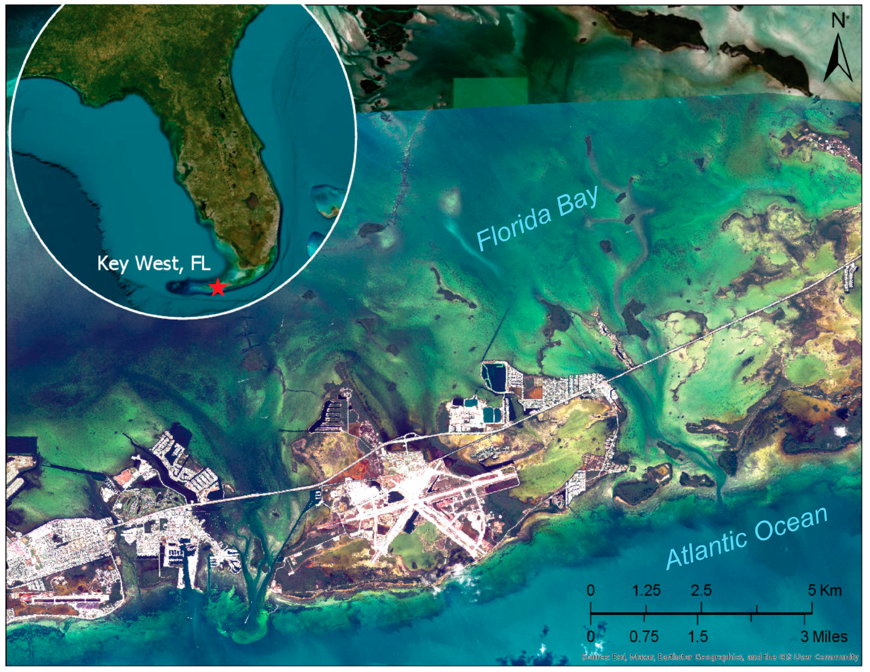
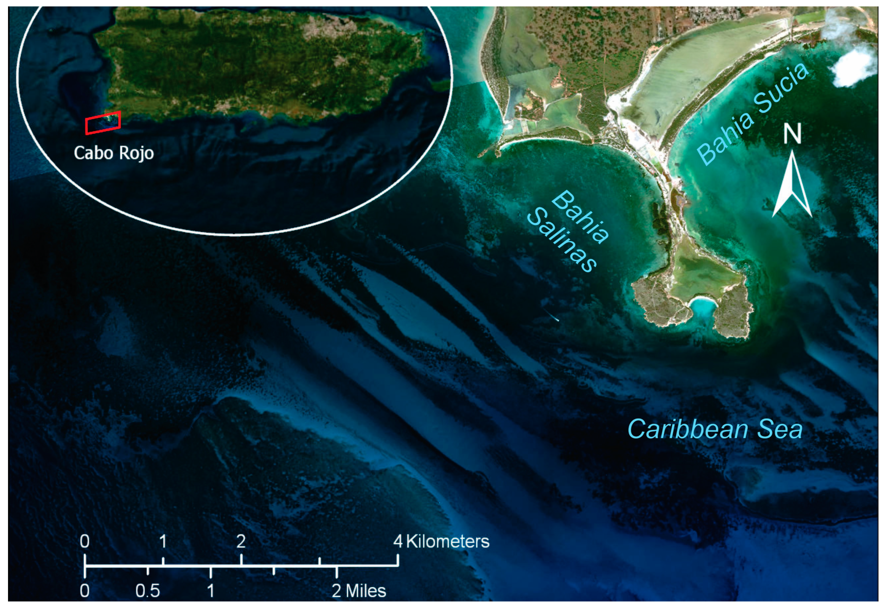
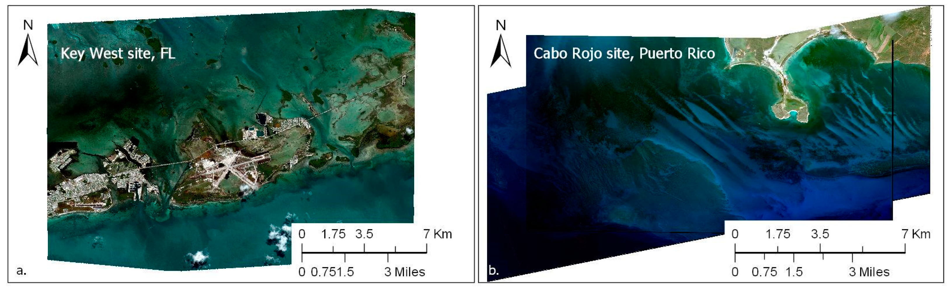
2.1. Study Sites
2.2. Datasets
2.2.1. WorldView Stereo Satellite Imagery
2.2.2. Lidar Data
- Florida Keys
- Puerto Rico
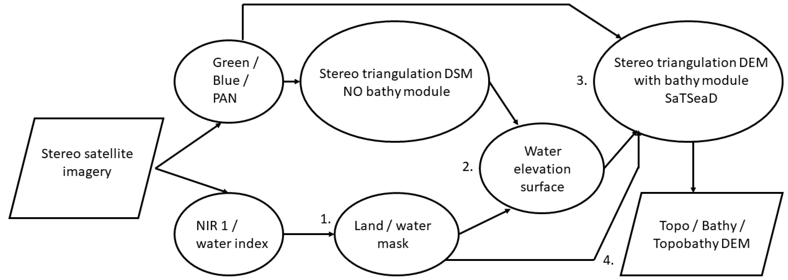
2.3. SaTSeaD Bathymetry Module
2.3.1. Using Only Satellite Stereo Imagery
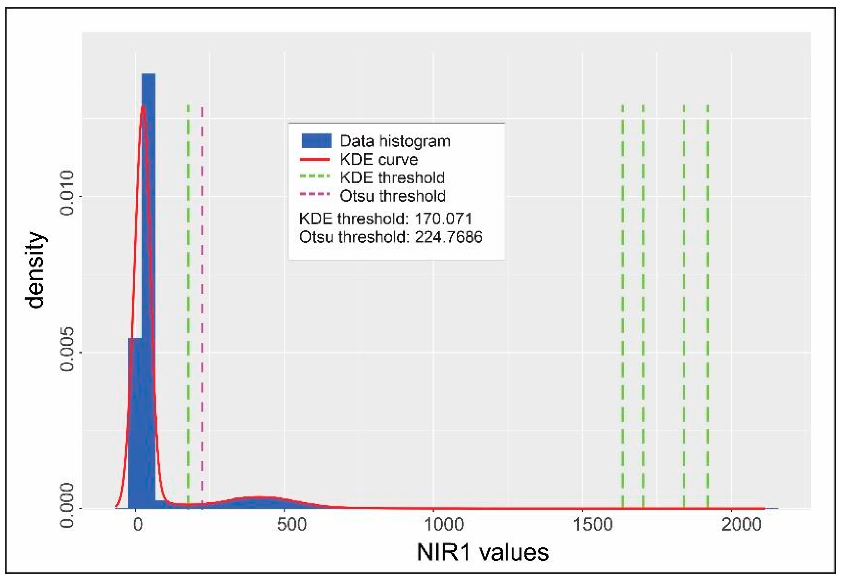
- Step 1. Land/water mask
- Step 2. Water elevation surface
- Method 1. External DEM, camera information, and land/water mask
- Method 2. Table with water height measurements
- Method 3. A DEM and a point shapefile
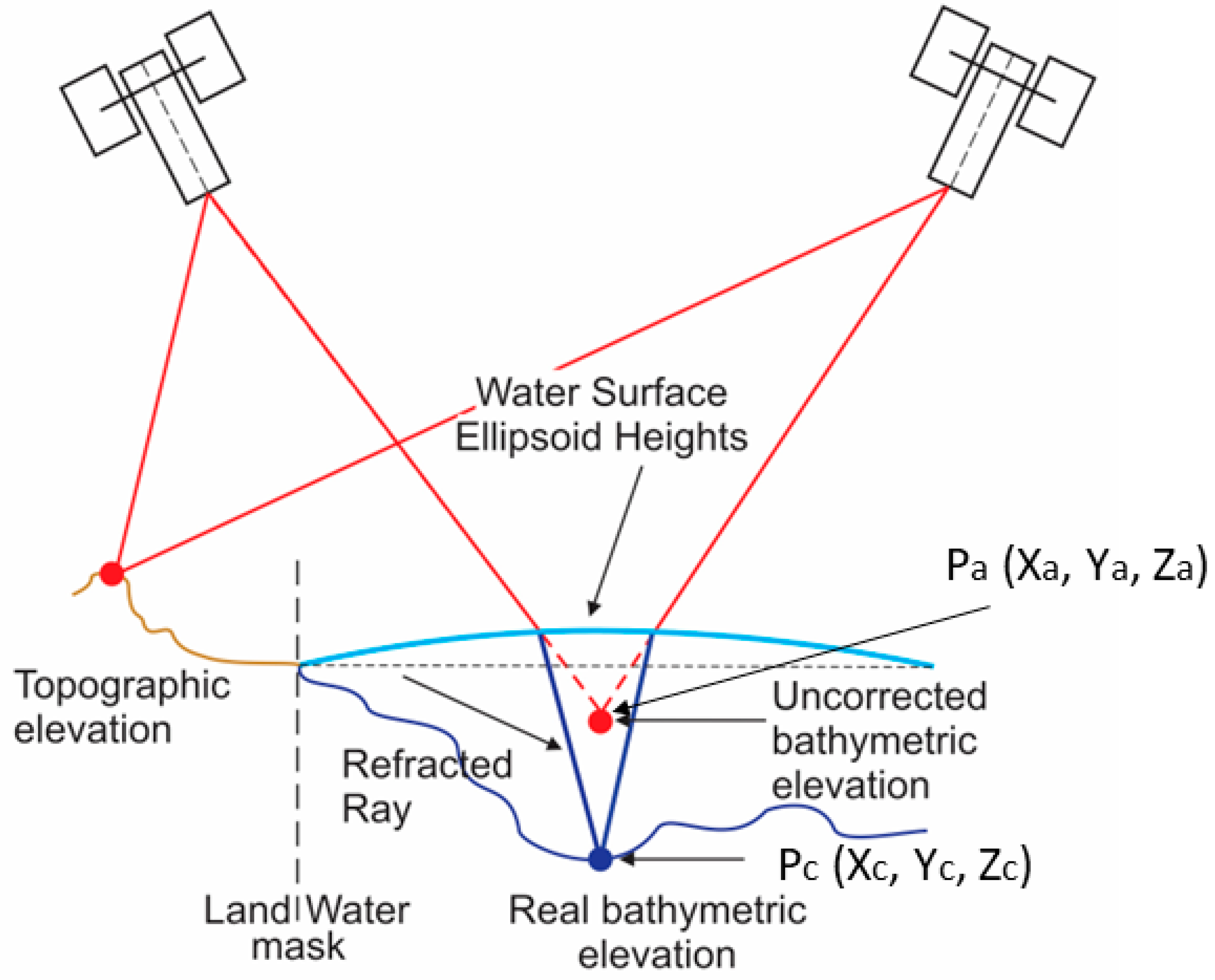
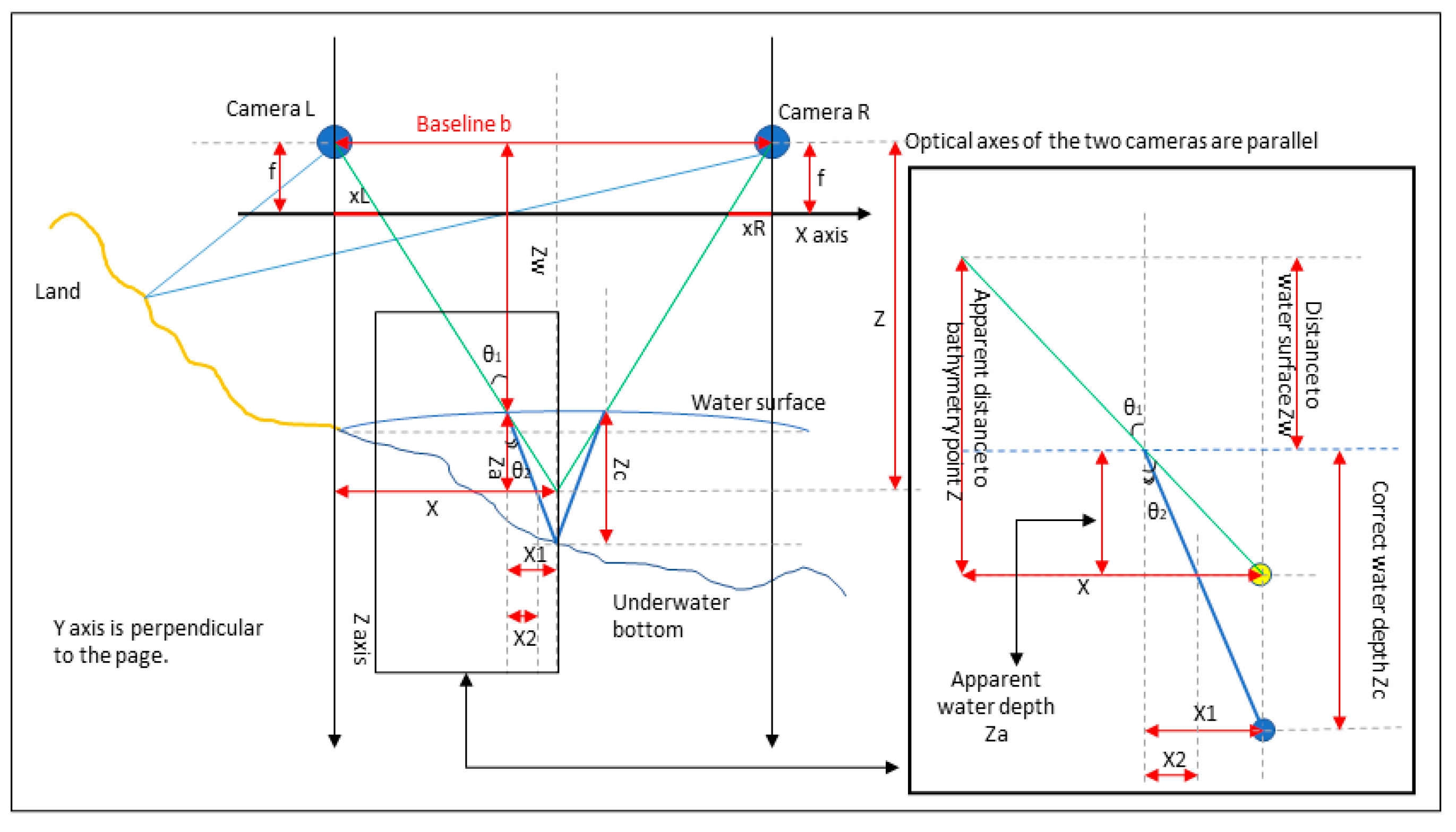
- Step 3. Stereo triangulation with bathymetry module
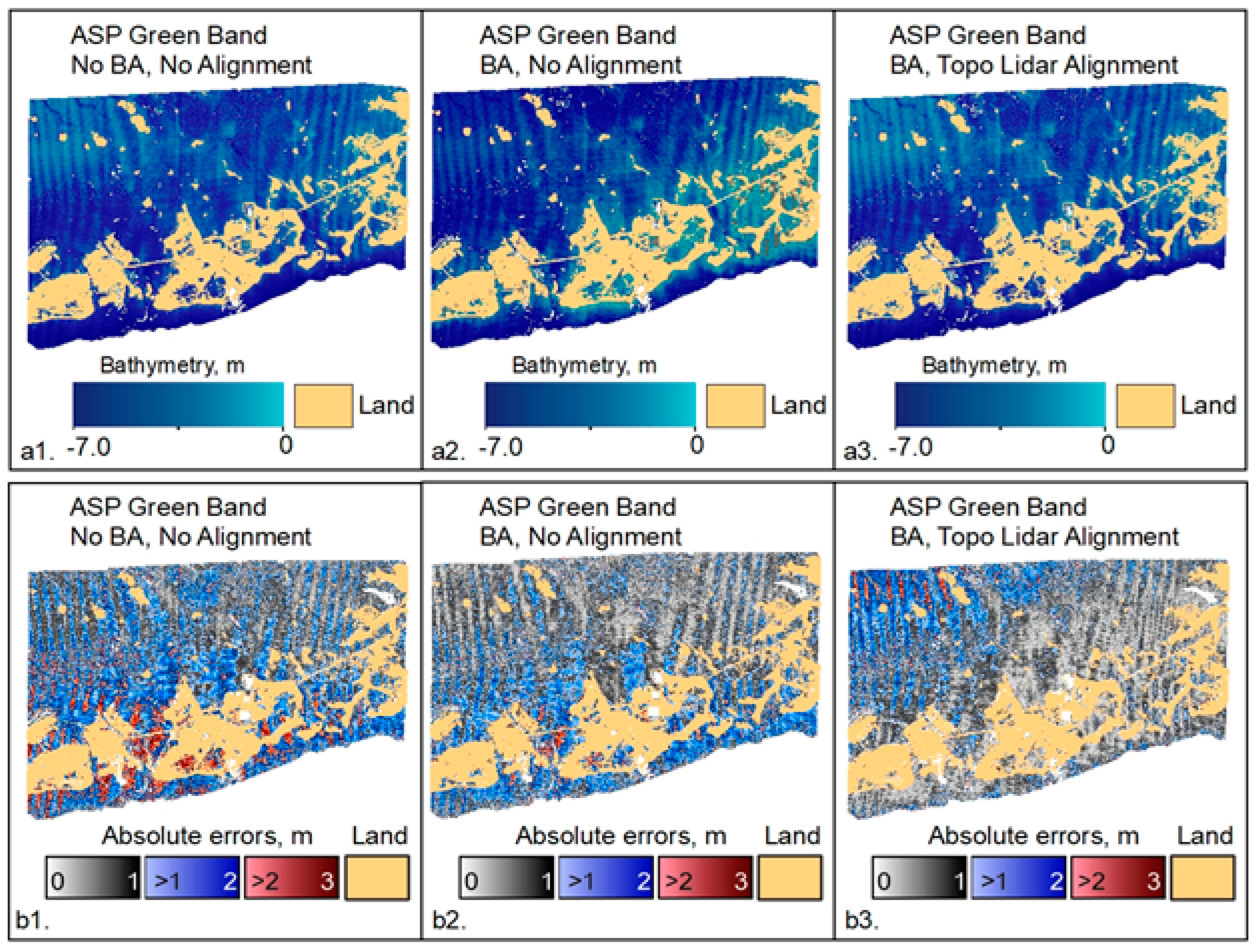
2.3.2. Using Bundle Adjustment and Panchromatic Stereo Bands
2.3.3. Alignment to External High-Accuracy Topography
3. Results
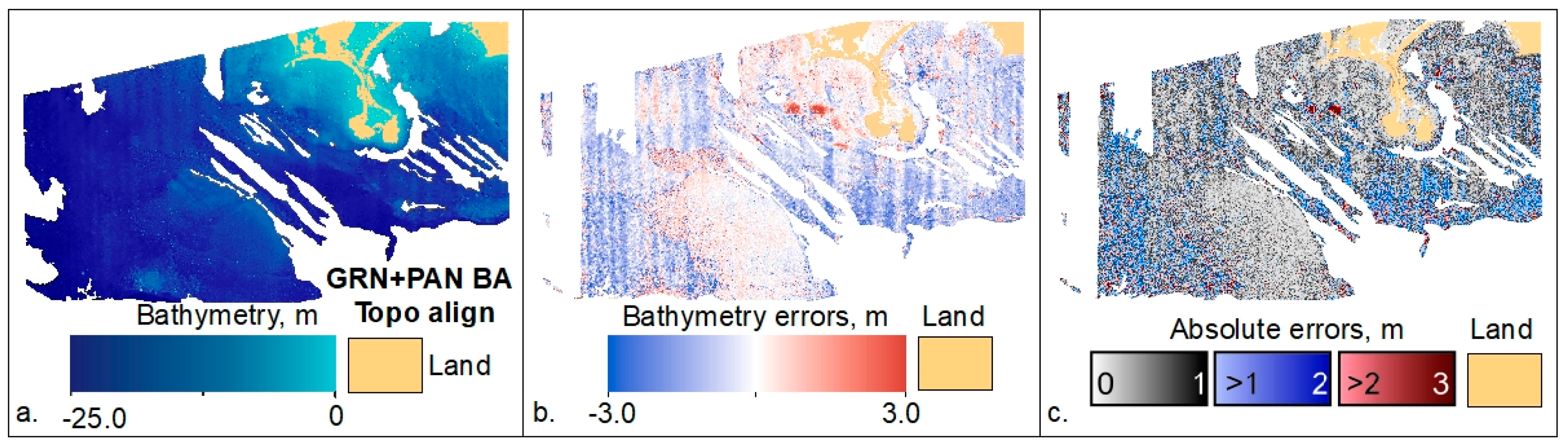
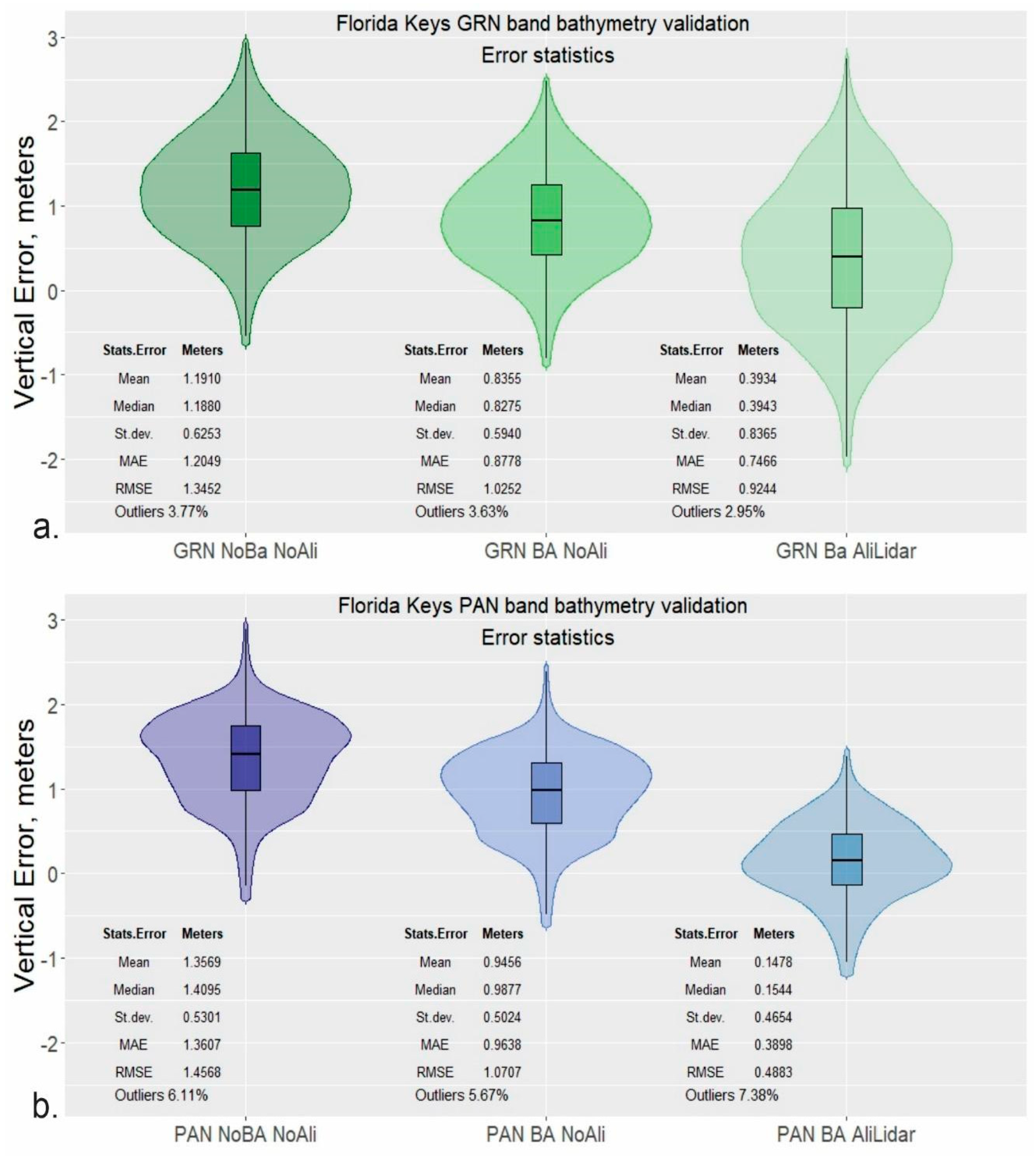
3.1. Florida Keys
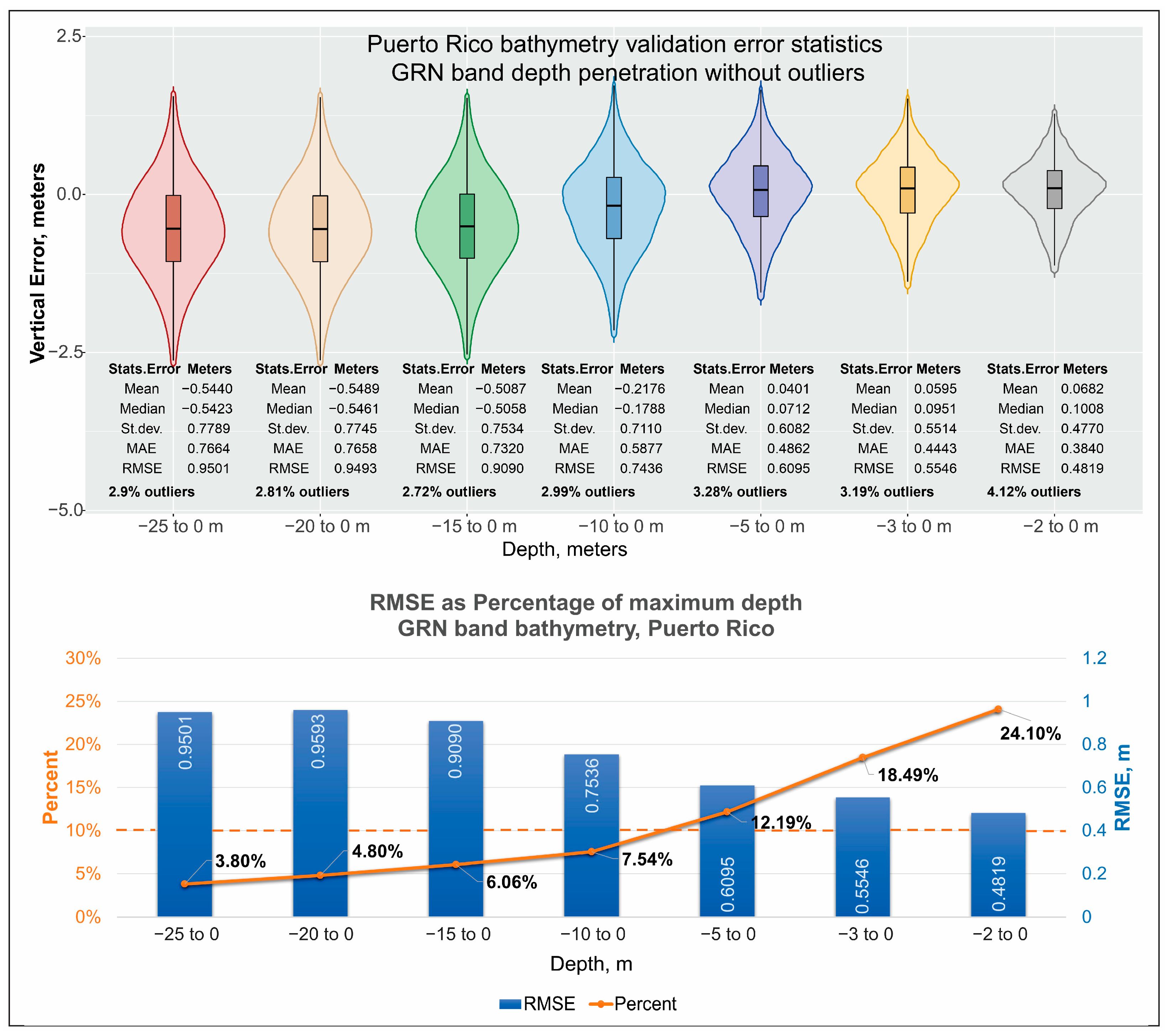
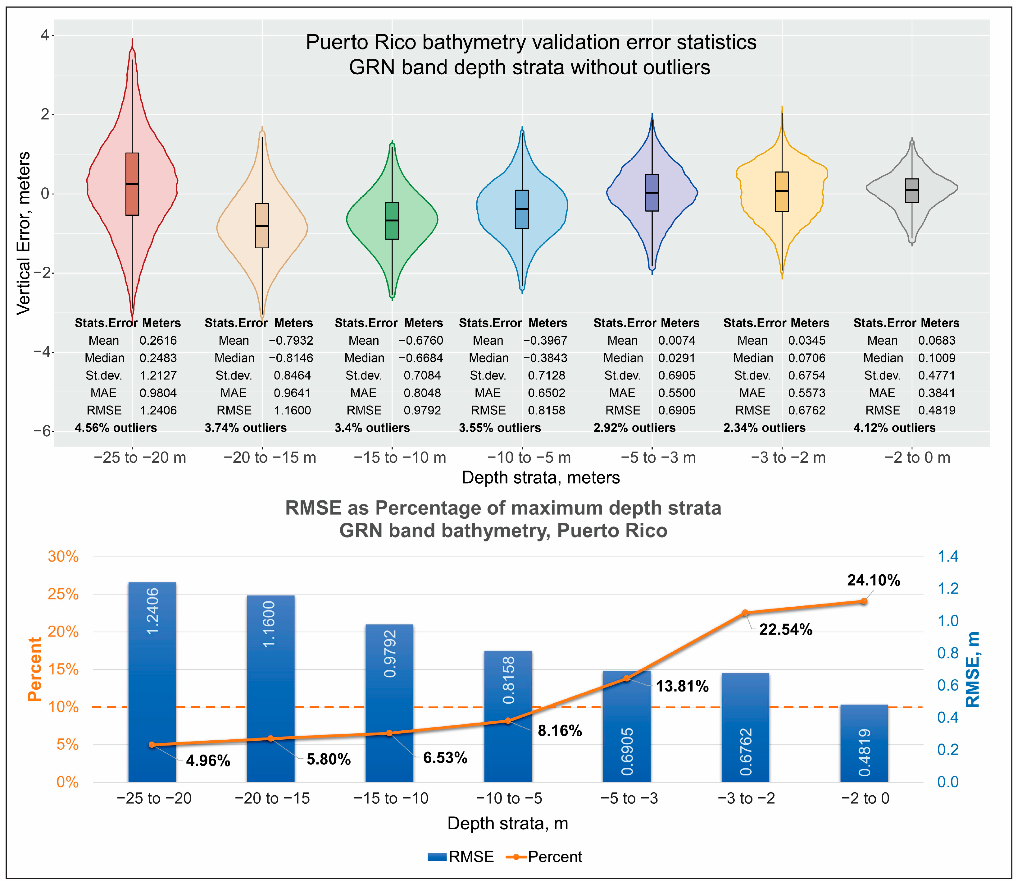
3.2. Cabo Rojo, Puerto Rico
4. Discussion
5. Conclusions
Author Contributions
Funding
Data Availability Statement
Acknowledgments
Conflicts of Interest
Disclaimers
References
- Ashphaq, M.; Srivastava, P.K.; Mitra, D. Review of near-shore satellite derived bathymetry: Classification and account of five decades of coastal bathymetry research. J. Ocean Eng. Sci. 2021, 6, 340–359. [Google Scholar] [CrossRef]
- Lyzenga, D.R. Passive remote sensing techniques for mapping water depth and bottom features. Appl. Opt. 1978, 17, 379–383. [Google Scholar] [CrossRef] [PubMed]
- Dunn, D.; Stewart, K.; Bjorkland, R.; Haughton, M.; Singh-Renton, S.; Lewison, R.; Thorne, L.; Halpin, P. A regional analysis of coastal and domestic fishing effort in the wider Caribbean. Fish. Res. 2010, 102, 60–68. [Google Scholar] [CrossRef]
- Foley, M.M.; Halpern, B.S.; Micheli, F.; Armsby, M.H.; Caldwell, M.R.; Crain, C.M.; Prahler, E.; Rohr, N.; Sivas, D.; Beck, M.W.; et al. Guiding ecological principles for marine spatial planning. Mar. Policy 2010, 34, 955–966. [Google Scholar] [CrossRef]
- Bell, J.D.; Albert, J.; Andréfouët, S.; Andrew, N.L.; Blanc, M.; Bright, P.; Brogan, D.; Campbell, B.; Govan, H.; Hampton, J.; et al. Optimising the use of nearshore fish aggregating devices for food security in the Pacific Islands. Mar. Policy 2015, 56, 98–105. [Google Scholar] [CrossRef]
- Flower, J.; Ramdeen, R.; Estep, A.; Thomas, L.R.; Francis, S.; Goldberg, G.; Johnson, A.E.; McClintock, W.; Mendes, S.R.; Mengerink, K.; et al. Marine spatial planning on the Caribbean island of Montserrat: Lessons for data-limited small islands. Conserv. Sci. Pract. 2020, 2, e158. [Google Scholar] [CrossRef]
- Parodi, M.U.; Giardino, A.; van Dongeren, A.; Pearson, S.G.; Bricker, J.D.; Reniers, A.J.H.M. Uncertainties in coastal flood risk assessments in small island developing states. Nat. Hazards Earth Syst. Sci. 2020, 20, 2397–2414. [Google Scholar] [CrossRef]
- Marks, K.M.; Smith, W.H.F. An Evaluation of Publicly Available Global Bathymetry Grids. Mar. Geophys. Res. 2006, 27, 19–34. [Google Scholar] [CrossRef]
- Becker, J.J.; Sandwell, D.T.; Smith, W.H.F.; Braud, J.; Binder, B.; Depner, J.; Fabre, D.; Factor, J.; Ingalls, S.; Kim, S.-H.; et al. Global Bathymetry and Elevation Data at 30 Arc Seconds Resolution: SRTM30_PLUS. Mar. Geod. 2009, 32, 355–371. [Google Scholar] [CrossRef]
- Tozer, B.; Sandwell, D.T.; Smith, W.H.F.; Olson, C.; Beale, J.R.; Wessel, P. Global Bathymetry and Topography at 15 Arc Sec: SRTM15+. Earth Space Sci. 2019, 6, 1847–1864. [Google Scholar] [CrossRef]
- Wölfl, A.-C.; Snaith, H.; Amirebrahimi, S.; Devey, C.W.; Dorschel, B.; Ferrini, V.; Huvenne, V.A.I.; Jakobsson, M.; Jencks, J.; Johnston, G.; et al. Seafloor Mapping—The Challenge of a Truly Global Ocean Bathymetry. Front. Mar. Sci. 2019, 6, 283. [Google Scholar] [CrossRef] [Green Version]
- European Marine Observation and Data Network (EMODnet). Available online: https://emodnet.ec.europa.eu/en (accessed on 19 May 2023).
- Nippon Foundation–GEBCO Seabed 2030 Project. Available online: https://seabed2030.gebco.net/ (accessed on 19 May 2023).
- International Hydrographic Organization (IHO) Data Center for Digital Bathymetry (IHO DCDB). Available online: https://iho.int/en/data-centre-for-digital-bathymetry (accessed on 19 May 2023).
- IHO Crowdsourced Bathymetry Initiative. Available online: https://iho.int/en/crowdsourced-bathymetry (accessed on 19 May 2023).
- Mayer, L.; Jakobsson, M.; Allen, G.; Dorschel, B.; Falconer, R.; Ferrini, V.; Lamarche, G.; Snaith, H.; Weatherall, P. The Nippon Foundation—GEBCO Seabed 2030 Project: The Quest to See the World’s Oceans Completely Mapped by 2030. Geosciences 2018, 8, 63. [Google Scholar] [CrossRef] [Green Version]
- International Hydrographic Organization (IHO). The IHO-IOC GEBCO Cook Book; IHO Publication B-11; IHO: Monte Carlo, Monaco, 2014; 331p, Available online: https://www.gebco.net/data_and_products/gebco_cook_book/ (accessed on 23 January 2021).
- Thierry, S.; Dick, S.; George, S.; Benoit, L.; Cyrille, P. EMODnet Bathymetry a compilation of bathymetric data in the European waters. In Proceedings of the OCEANS 2019—Marseille, Marseille, France, 17–20 June 2019; pp. 1–7. [Google Scholar] [CrossRef]
- Ferrini, V. Assembling the Bathymetric Puzzle to Create a Global Ocean Map. Mar. Technol. Soc. J. 2020, 54, 13–17. [Google Scholar] [CrossRef]
- Westington, M.; Varner, J.; Johnson, P.; Sutherland, M.; Armstrong, A.; Jencks, J. Assessing Sounding Density for a Seabed 2030 Initiative. In Proceedings of the Canadian Hydrographic Conference, Victoria, BC, Canada, 26–29 March 2018; Available online: https://na.eventscloud.com/file_uploads/88d4852d59327aec9aee1f08b5f64e84_AssessingSoundingDensityforaSeabed2030Initiative_CHC20181Meredith.pdf (accessed on 3 April 2023).
- Landsat Archive Became Freely Available in 2008. USGS News. Available online: https://www.usgs.gov/media/files/2008-free-landsat-image-archive-news-release (accessed on 3 April 2023).
- Sentinel-2A. Available online: https://sentinel.esa.int/web/sentinel/sentinel-data-access (accessed on 3 April 2023).
- Stumpf, R.P.; Holderied, K.; Sinclair, M. Determination of water depth with high-resolution satellite imagery over variable bottom types. Limnol. Oceanogr. 2003, 48, 547–556. [Google Scholar] [CrossRef]
- Lyzenga, D.; Malinas, N.; Tanis, F. Multispectral bathymetry using a simple physically based algorithm. IEEE Trans. Geosci. Remote Sens. 2006, 44, 2251–2259. [Google Scholar] [CrossRef]
- Pe’eri, S.; Azuike, C.; Alexander, L.; Parrish, C.; Armstrong, A. Beyond the Chart: The use of Satellite Remote Sensing for Assessing the Adequacy and Completeness Information. In Proceedings of the Canadian Hydrographic Conference, Quebec City, QC, Canada, 12–14 May 2012; p. 816. Available online: https://scholars.unh.edu/ccom/816 (accessed on 3 April 2023).
- Pe’eri, S.; Azuike, C.; Parrish, C. Satellite-Derived Bathymetry a Reconnaissance Tool for Hydrography. Hydro International. 1119. 2013. Available online: https://scholars.unh.edu/ccom/1119 (accessed on 3 April 2023).
- Caballero, I.; Stumpf, R.P. Retrieval of nearshore bathymetry from Sentinel-2A and 2B satellites in South Florida coastal waters. Estuar. Coast. Shelf Sci. 2019, 226, 106277. [Google Scholar] [CrossRef]
- Caballero, I.; Stumpf, R.P.; Meredith, A. Preliminary Assessment of Turbidity and Chlorophyll Impact on Bathymetry Derived from Sentinel-2A and Sentinel-3A Satellites in South Florida. Remote Sens. 2019, 11, 645. [Google Scholar] [CrossRef] [Green Version]
- Casal, G.; Monteys, X.; Hedley, J.; Harris, P.; Cahalane, C.; McCarthy, T. Assessment of empirical algorithms for bathymetry extraction using Sentinel-2 data. Int. J. Remote Sens. 2018, 40, 2855–2879. [Google Scholar] [CrossRef]
- Pike, S.; Traganos, D.; Poursanidis, D.; Williams, J.; Medcalf, K.; Reinartz, P.; Chrysoulakis, N. Leveraging Commercial High-Resolution Multispectral Satellite and Multibeam Sonar Data to Estimate Bathymetry: The Case Study of the Caribbean Sea. Remote Sens. 2019, 11, 1830. [Google Scholar] [CrossRef] [Green Version]
- Freire, R.; Pe’eri, S.; Madore, B.; Rzhanov, Y.; Alexander, L.; Parrish, C.E.; Lippmann, T.C. Monitoring Near-Shore Bathymetry Using a Multi-Image Satellite-Derived Bathymetry Approach. US Hydrographic Conference 2015. 2015. Available online: https://scholars.unh.edu/cgi/viewcontent.cgi?article=1011&context=ccom (accessed on 3 April 2023).
- Pe’Eri, S.; Madore, B.; Nyberg, J.; Snyder, L.; Parrish, C.; Smith, S. Identifying Bathymetric Differences over Alaska’s North Slope using a Satellite-derived Bathymetry Multi-temporal Approach. J. Coast. Res. 2016, 76, 56–63. [Google Scholar] [CrossRef]
- Caballero, I.; Stumpf, R.P. Atmospheric correction for satellite-derived bathymetry in the Caribbean waters: From a single image to multi-temporal approaches using Sentinel-2A/B. Opt. Express 2020, 28, 11742–11766. [Google Scholar] [CrossRef]
- Caballero, I.; Stumpf, R.P. Towards Routine Mapping of Shallow Bathymetry in Environments with Variable Turbidity: Contribution of Sentinel-2A/B Satellites Mission. Remote Sens. 2020, 12, 451. [Google Scholar] [CrossRef] [Green Version]
- Manessa, M.D.M.; Kanno, A.; Sekine, M.; Haidar, M.; Yamamoto, K.; Imai, T.; Higuchi, T. Satellite-derived bathymetry using random forest algorithm and worldview-2 imagery. Geoplan. J. Geomat. Plan. 2016, 3, 117–126. [Google Scholar] [CrossRef] [Green Version]
- Poursanidis, D.; Traganos, D.; Chrysoulakis, N.; Reinartz, P. Cubesats Allow High Spatiotemporal Estimates of Satellite-Derived Bathymetry. Remote Sens. 2019, 11, 1299. [Google Scholar] [CrossRef] [Green Version]
- Qayyum, N.; Ghuffar, S.; Ahmad, H.M.; Yousaf, A.; Shahid, I. Glacial Lakes Mapping Using Multi Satellite PlanetScope Imagery and Deep Learning. ISPRS Int. J. Geo-Inf. 2020, 9, 560. [Google Scholar] [CrossRef]
- Evagorou, E.; Argyriou, A.; Papadopoulos, N.; Mettas, C.; Alexandrakis, G.; Hadjimitsis, D. Evaluation of Satellite-Derived Bathymetry from High and Medium-Resolution Sensors Using Empirical Methods. Remote Sens. 2022, 14, 772. [Google Scholar] [CrossRef]
- Le Quilleuc, A.; Collin, A.; Jasinski, M.F.; Devillers, R. Very High-Resolution Satellite-Derived Bathymetry and Habitat Mapping Using Pleiades-1 and ICESat-2. Remote Sens. 2021, 14, 133. [Google Scholar] [CrossRef]
- Casal, G.; Harris, P.; Monteys, X.; Hedley, J.; Cahalane, C.; McCarthy, T. Understanding satellite-derived bathymetry using Sentinel 2 imagery and spatial prediction models. GISci. Remote Sens. 2019, 57, 271–286. [Google Scholar] [CrossRef]
- Vinayaraj, P.; Raghavan, V.; Masumoto, S. Satellite-Derived Bathymetry using Adaptive Geographically Weighted Regression Model. Mar. Geod. 2016, 39, 458–478. [Google Scholar] [CrossRef]
- Zhang, J.-Y.; Zhang, J.; Ma, Y.; Chen, A.-N.; Cheng, J.; Wan, J.-X. Satellite-derived bathymetry model in the Arctic waters based on support vector regression. J. Coast. Res. 2019, 90, 294–301. [Google Scholar] [CrossRef]
- Said, N.M.; Mahmud, M.R.; Hasan, R.C. Satellite-Derived Bathymetry: Accuracy Assessment On Depths Derivation Algorithm For Shallow Water Area. ISPRS—Int. Arch. Photogramm. Remote Sens. Spat. Inf. Sci. 2017, XLII-4/W5, 159–164. [Google Scholar] [CrossRef] [Green Version]
- Manessa, M.D.M.; Setiawan, K.T.; Haidar, M.; Supriatna, S.; Pataropura, A.; Supardjo, A.H. Optimization of the Random Forest Algorithm for Multispectral Derived Bathymetry. Int. J. Geoinform. 2020, 16, 1–6. [Google Scholar]
- El-Diasty, M. Satellite-Based Bathymetric Modeling Using a Wavelet Network Model. ISPRS Int. J. Geo-Inf. 2019, 8, 405. [Google Scholar] [CrossRef] [Green Version]
- Sagawa, T.; Yamashita, Y.; Okumura, T.; Yamanokuchi, T. Satellite Derived Bathymetry Using Machine Learning and Multi-Temporal Satellite Images. Remote Sens. 2019, 11, 1155. [Google Scholar] [CrossRef] [Green Version]
- Tonion, F.; Pirotti, F.; Faina, G.; Paltrinieri, D. A machine learning approach to multispectral satellite derived bathymetry. ISPRS Ann. Photogramm. Remote Sens. Spat. Inf. Sci. 2020, 3, 565–570. [Google Scholar] [CrossRef]
- Wilson, B.; Kurian, N.C.; Singh, A.; Sethi, A. Satellite-Derived Bathymetry Using Deep Convolutional Neural Network. In Proceedings of the IGARSS 2020 IEEE International Geoscience and Remote Sensing Symposium, Waikoloa, HI, USA, 26 September–2 October 2020; pp. 2280–2283. [Google Scholar] [CrossRef]
- Wiehle, S.; Pleskachevsky, A.; Gebhardt, C. Automatic bathymetry retrieval from SAR images. CEAS Space J. 2019, 11, 105–114. [Google Scholar] [CrossRef] [Green Version]
- Santos, D.; Fernández-Fernández, S.; Abreu, T.; Silva, P.A.; Baptista, P. Retrieval of nearshore bathymetry from Sentinel-1 SAR data in high energetic wave coasts: The Portuguese case study. Remote Sens. Appl. Soc. Environ. 2021, 25, 100674. [Google Scholar] [CrossRef]
- Daly, C.J.; Baba, W.; Bergsma, E.; Almar, R.; Garlan, T. The New Era of Regional Coastal Bathymetry from Space: A Showcase for West Africa using Sentinel-2Imagery. arXiv 2020. [Google Scholar] [CrossRef]
- Almar, R.; Bergsma, E.W.J.; Thoumyre, G.; Baba, M.W.; Cesbron, G.; Daly, C.; Garlan, T.; Lifermann, A. Global Satellite-Based Coastal Bathymetry from Waves. Remote Sens. 2021, 13, 4628. [Google Scholar] [CrossRef]
- Casal, G.; Hedley, J.D.; Monteys, X.; Harris, P.; Cahalane, C.; McCarthy, T. Satellite-derived bathymetry in optically complex waters using a model inversion approach and Sentinel-2 data. Estuar. Coast. Shelf Sci. 2020, 241, 106814. [Google Scholar] [CrossRef]
- Markus, T.; Neumann, T.; Martino, A.; Abdalati, W.; Brunt, K.; Csatho, B.; Farrell, S.; Fricker, H.; Gardner, A.; Harding, D.; et al. The Ice, Cloud, and land Elevation Satellite-2 (ICESat-2): Science requirements, concept, and implementation. Remote Sens. Environ. 2017, 190, 260–273. [Google Scholar] [CrossRef]
- Parrish, C.E.; Magruder, L.A.; Neuenschwander, A.L.; Forfinski-Sarkozi, N.; Alonzo, M.; Jasinski, M. Validation of ICESat-2 ATLAS Bathymetry and Analysis of ATLAS’s Bathymetric Mapping Performance. Remote Sens. 2019, 11, 1634. [Google Scholar] [CrossRef] [Green Version]
- Walker, M.; Magruder, L.A.; Neuenschwander, A.L.; Klotz, B. Satellite Computed Bathymetry Assessment-SCuBA. In Proceedings of the American Geophysical Union, Fall Meeting 2020, Virtual, 1–17 December 2020. [Google Scholar]
- Albright, A.; Glennie, C. Nearshore Bathymetry From Fusion of Sentinel-2 and ICESat-2 Observations. IEEE Geosci. Remote Sens. Lett. 2020, 18, 900–904. [Google Scholar] [CrossRef]
- Ma, Y.; Xu, N.; Liu, Z.; Yang, B.; Yang, F.; Wang, X.H.; Li, S. Satellite-derived bathymetry using the ICESat-2 lidar and Sentinel-2 imagery datasets. Remote Sens. Environ. 2020, 250, 112047. [Google Scholar] [CrossRef]
- Babbel, B.J.; Parrish, C.E.; Magruder, L.A. ICESat-2 Elevation Retrievals in Support of Satellite-Derived Bathymetry for Global Science Applications. Geophys. Res. Lett. 2021, 48, e2020GL090629. [Google Scholar] [CrossRef]
- Thomas, N.; Pertiwi, A.P.; Traganos, D.; Lagomasino, D.; Poursanidis, D.; Moreno, S.; Fatoyinbo, L. Space-Borne Cloud-Native Satellite-Derived Bathymetry (SDB) Models Using ICESat-2 And Sentinel-2. Geophys. Res. Lett. 2021, 48, e2020GL092170. [Google Scholar] [CrossRef]
- Xu, N.; Ma, Y.; Zhou, H.; Zhang, W.; Zhang, Z.; Wang, X.H. A Method to Derive Bathymetry for Dynamic Water Bodies Using ICESat-2 and GSWD Data Sets. IEEE Geosci. Remote Sens. Lett. 2022, 19, 1–5. [Google Scholar] [CrossRef]
- Li, S.; Wang, X.H.; Ma, Y.; Yang, F. Satellite-Derived Bathymetry with Sediment Classification Using ICESat-2 and Multispectral Imagery: Case Studies in the South China Sea and Australia. Remote Sens. 2023, 15, 1026. [Google Scholar] [CrossRef]
- Kerr, J.M.; Purkis, S. An algorithm for optically-deriving water depth from multispectral imagery in coral reef landscapes in the absence of ground-truth data. Remote Sens. Environ. 2018, 210, 307–324. [Google Scholar] [CrossRef]
- Hodúl, M.; Bird, S.; Knudby, A.; Chénier, R. Satellite derived photogrammetric bathymetry. ISPRS J. Photogramm. Remote Sens. 2018, 142, 268–277. [Google Scholar] [CrossRef]
- Hodúl, M.; Chénier, R.; Faucher, M.-A.; Ahola, R.; Knudby, A.; Bird, S. Photogrammetric Bathymetry for the Canadian Arctic. Mar. Geod. 2019, 43, 23–43. [Google Scholar] [CrossRef] [Green Version]
- Cao, B.; Fang, Y.; Jiang, Z.; Gao, L.; Hu, H. Shallow water bathymetry from WorldView-2 stereo imagery using two-media photogrammetry. Eur. J. Remote Sens. 2019, 52, 506–521. [Google Scholar] [CrossRef] [Green Version]
- Blake, S. A Multi-Spatial, Multi-Temporal, Semi-Analytical Model for Bathymetry, Water Turbidity and Bottom Composition using Multispectral Imagery. Electrical Engineering and Systems Science Signal Processing. arXiv 2020, arXiv:2002.02298. [Google Scholar]
- Blake, S. Photic—A Physics-Based, Satellite-Derived Bathymetry Model. 2020. Available online: https://github.com/geo-py/satellite_derived_bathymetry_model (accessed on 3 April 2023).
- Thomas, N.; Lee, B.; Coutts, O.; Bunting, P.; Lagomasino, D.; Fatoyinbo, L. A Purely Spaceborne Open Source Approach for Regional Bathymetry Mapping. IEEE Trans. Geosci. Remote Sens. 2022, 60, 1–9. [Google Scholar] [CrossRef]
- Bunting, P.; Clewley, D.; Lucas, R.M.; Gillingham, S. The Remote Sensing and GIS Software Library (RSGISLib). Comput. Geosci. 2014, 62, 216–226. [Google Scholar] [CrossRef]
- Gege, P. WASI-2D: A software tool for regionally optimized analysis of imaging spectrometer data from deep and shallow waters. Comput. Geosci. 2014, 62, 208–215. [Google Scholar] [CrossRef] [Green Version]
- Alevizos, E.; Le Bas, T.; Alexakis, D.D. Assessment of PRISMA Level-2 Hyperspectral Imagery for Large Scale Satellite-Derived Bathymetry Retrieval. Mar. Geod. 2022, 45, 251–273. [Google Scholar] [CrossRef]
- NASA Ames Stereo Pipeline 3.2.0 Documentation Section 8.27. Shallow-Water Bathymetry. Available online: https://stereopipeline.readthedocs.io/en/latest/examples/bathy.html (accessed on 3 April 2023).
- Shean, D.E.; Alexandrov, O.; Moratto, Z.M.; Smith, B.E.; Joughin, I.R.; Porter, C.; Morin, P. An automated, open-source pipeline for mass production of digital elevation models (DEMs) from very-high-resolution commercial stereo satellite imagery. ISPRS J. Photogramm. Remote Sens. 2016, 116, 101–117. [Google Scholar] [CrossRef]
- Beyer, R.A.; Alexandrov, O.; McMichael, S. The Ames Stereo Pipeline: NASA’s Open Source Software for Deriving and Processing Terrain Data. Earth Space Sci. 2018, 5, 537–548. [Google Scholar] [CrossRef]
- NASA Ames Stereo Pipeline 3.2.0 Documentation. Available online: https://stereopipeline.readthedocs.io/en/latest/ (accessed on 3 April 2023).
- NASA Ames Stereo Pipeline Daily Release. Available online: https://github.com/NeoGeographyToolkit/StereoPipeline/releases (accessed on 3 April 2023).
- NASA Ames Stereo Pipeline 3.2.0 Stable Release. Available online: https://doi.org/10.5281/zenodo.7497499 (accessed on 3 April 2023).
- Halley, R.B.; Vacher, H.; Shinn, E.A. Geology and Hydrogeology of the Florida Keys. Dev. Sedimentol. 2004, 54, 217–248. [Google Scholar] [CrossRef]
- Volckmann, R. Geologic map of the Cabo Rojo and Parguera quadrangles, southwest Puerto Rico. USGS IMAP 1557 1984. [Google Scholar] [CrossRef]
- Schlee, J.; Rodriguez, R.; Webb, R.; Carlo, M. Marine geologic map of the southwestern insular shelf of Puerto Rico, Mayaguez to Cabo Rojo. USFS IMAP 2615 1999. [Google Scholar] [CrossRef] [Green Version]
- Prada, M.C.; Appeldoorn, R.S.; Rivera, J.A. Improving Coral Reef Habitat Mapping of the Puerto Rico Insular Shelf Using Side Scan Sonar. Mar. Geod. 2008, 31, 49–73. [Google Scholar] [CrossRef]
- USGS (United States Geological Survey). Available online: https://earthexplorer.usgs.gov (accessed on 10 June 2017).
- NOAA National Geodetic Survey. 2018–2019 NOAA NGS Topobathy Lidar Hurricane Irma: Miami to Marquesas Keys, FL. 2020. Available online: https://www.fisheries.noaa.gov/inport/item/63017 (accessed on 3 April 2023).
- OCM Partners. 2018 USACE FEMA Topobathy Lidar: Main Island, Culebra, and Vieques, Puerto Rico. 2020. Available online: https://www.fisheries.noaa.gov/inport/item/53078 (accessed on 3 April 2023).
- NOAA National Geodetic Survey. 2019 NOAA NGS Topobathy Lidar: Puerto Rico. 2020. Available online: https://www.fisheries.noaa.gov/inport/item/65546 (accessed on 3 April 2023).
- NASA Ames Stereo Pipeline 3.2.0 Documentation, Section 16.4. bathy_threshold_calc.py. Available online: https://stereopipeline.readthedocs.io/en/latest/tools/bathy_threshold_calc.html#bathy-threshold-calc (accessed on 3 April 2023).
- NASA Ames Stereo Pipeline 3.2.0 Documentation Section 16.41. otsu_threshold. Available online: https://stereopipeline.readthedocs.io/en/latest/tools/otsu_threshold.html#otsu-threshold (accessed on 3 April 2023).
- Otsu, N. A threshold selection method from gray-level histograms. IEEE Trans. Syst. Man Cybern. 1979, 9, 62–66. [Google Scholar] [CrossRef] [Green Version]
- NASA Ames Stereo Pipeline 3.2.0 Documentation Section 16.3. bathy_plane_calc. Available online: https://stereopipeline.readthedocs.io/en/latest/tools/bathy_plane_calc.html#bathy-plane-calc (accessed on 3 April 2023).
- NOAA Vertical Datum Transformation. Available online: https://vdatum.noaa.gov/welcome.html (accessed on 24 May 2021).
- Jerlov, N.G. Marine Optics; Elsevier Scientific Pub. Co.: Amsterdam, The Netherlands, 1976; p. 231. [Google Scholar]
- Harvey, E.S.; Shortis, M.R. Calibration stability of an underwater stereo-video system: Implications for measurement accuracy and precision. Mar. Technol. Soc. J. 1998, 32, 3–17. [Google Scholar]
- Thormählen, I.; Straub, J.; Grigull, U. Refractive Index of Water and Its Dependence on Wavelength, Temperature, and Density. J. Phys. Chem. Ref. Data 1985, 14, 933–945. [Google Scholar] [CrossRef] [Green Version]
- Austin, R.W.; Halikas, G. The Index of Refraction of Seawater; SIO Ref. No. 76-1; Scripps Institution of Oceanography: San Diego, CA, USA, 1976. [Google Scholar] [CrossRef] [Green Version]
- Mobley, C.D. The Optical Properties of Water. In Handbook of Optics; Bass, M., Ed.; McGraw-Hill: New York, NY, USA, 1995. [Google Scholar]
- Parrish, C. Index of Refraction of Seawater and Freshwater as a Function of Wavelength and Temperature. 2020. Available online: https://research.engr.oregonstate.edu/parrish/index-refraction-seawater-and-freshwater-function-wavelength-and-temperature (accessed on 14 April 2023).
- Murase, T.; Tanaka, M.; Tani, T.; Miyashita, Y.; Ohkawa, N.; Ishiguro, S.; Suzuki, Y.; Kayanne, H.; Yamano, H. A Photogrammetric Correction Procedure for Light Refraction Effects at a Two-Medium Boundary. Photogramm. Eng. Remote Sens. 2007, 73, 1129–1136. [Google Scholar] [CrossRef]
- NASA Ames Stereo Pipeline 3.2.0 Documentation Section 16.5. bundle_adjust. Available online: https://stereopipeline.readthedocs.io/en/latest/tools/bundle_adjust.html#bundle-adjust (accessed on 14 April 2023).
- Pomerleau, F.; Colas, F.; Siegwart, R.; Magnenat, S. Comparing ICP variants on real-world data sets: Open-source library and experimental protocol. Auton. Robot. 2013, 34, 133–148. [Google Scholar] [CrossRef]
- NASA Ames Stereo Pipeline 3.2.0 Documentation Section 16.47. pc_align. Available online: https://stereopipeline.readthedocs.io/en/latest/tools/pc_align.html#alignment-method (accessed on 14 April 2023).
- Zhou, Q.-Y.; Park, J.; Koltun, V. Fast Global Registration. In Computer Vision—ECCV 2016; ECCV 2016, Lecture Notes in Computer Science; Leibe, B., Matas, J., Sebe, N., Welling, M., Eds.; Springer: Cham, Switzerland, 2016; Volume 9906. [Google Scholar]
- Copernicus Global 30 m. Available online: https://spacedata.copernicus.eu/fr/collections/copernicus-digital-elevation-model (accessed on 14 April 2023).
- ICESat-2 Data. Available online: https://www.earthdata.nasa.gov/learn/find-data/near-real-time/icesat2-nrt (accessed on 14 April 2023).
- NASA Ames Stereo Pipeline 3.2.0 Documentation Section 16.34 jitter_solve. Available online: https://stereopipeline.readthedocs.io/en/latest/tools/jitter_solve.html (accessed on 17 July 2023).
- NASA Ames Stereo Pipeline 3.2.0 Documentation Section 16.67 wv_correct. Available online: https://stereopipeline.readthedocs.io/en/latest/tools/wv_correct.html (accessed on 17 July 2023).
- Hintze, J.L.; Nelson, R.D. Violin Plots: A Box Plot-Density Trace Synergism. Am. Stat. 1998, 52, 181–184. [Google Scholar]
- Tukey, J.W. Exploratory Data Analysis; Addison-Wesley Pub. Co.: Abingdon, UK, 1977. [Google Scholar]
- The Interagency Working Group on Ocean and Coastal Mapping. National Coastal Mapping Strategy 1.0: Coastal LIDAR Elevation for a 3D Nation. 2018. Available online: https://iocm.noaa.gov/about/documents/strategic-plans/IWG-OCM-Final-Coastal-Mapping-Strategy-2018-with-cover.pdf (accessed on 21 April 2023).


| Site | Imagery | Date | Stereo Convergence Angle (Degrees) | |
|---|---|---|---|---|
| Match Points | Angle | |||
| Key West, FL | WV-2 | 01/05/2015 | 576 | 34.51 |
| Cabo Rojo, PR | WV-3 | 25/02/2022 | 241 | 31.15 |
| Left Mask | |||
| Mask Type, Parameters | WGS 1994 Ellipsoid, m | Mask Type, Parameters | WGS 1994 Ellipsoid, m |
| Otsu 0.2, 30 k | −23.8932 | KDE 0.2, 30 k | −23.9418 |
| Otsu 0.2, 300 k | −24.1428 | KDE 0.2, 300 k | −23.9519 |
| Otsu 0.5, 30 k | −24.0526 | KDE 0.5, 30 k | −24.0496 |
| Otsu 0.5, 300 k | −23.922 | KDE 0.5, 300 k | −23.9244 |
| Right mask | |||
| Mask type, parameters | WGS 1994 ellipsoid, m | Mask type, parameters | WGS 1994 ellipsoid, m |
| Otsu 0.2, 30 k | −23.9379 | KDE 0.2, 30 k | −23.9004 |
| Otsu 0.2, 300 k | −23.9379 | KDE 0.2, 300 k | −23.9221 |
| Otsu 0.5, 30 k | −24.0316 | KDE 0.5, 30 k | −24.0849 |
| Otsu 0.5, 300 k | −23.9959 | KDE 0.5, 300 k | −24.0187 |
| Statistics | Initial (Meters) | BA (Meters) | BA, TAli (Meters) | Differences (Meters) | ||
|---|---|---|---|---|---|---|
| Initial vs. BA | Initial vs. BA, TAli | BA vs. BA, TAli | ||||
| Mean | 1.1910 | 0.8355 | 0.3934 | 0.3555 | 0.7976 | 0.4421 |
| Median | 1.1880 | 0.8275 | 0.3943 | 0.3605 | 0.7937 | 0.4332 |
| St. Dev. | 0.6253 | 0.5940 | 0.8365 | 0.0313 | −0.2112 | −0.2425 |
| MAE | 1.2049 | 0.8778 | 0.7466 | 0.3271 | 0.4583 | 0.1312 |
| RMSE | 1.3452 | 1.0252 | 0.9244 | 0.3200 | 0.4208 | 0.1008 |
| Statistics | Initial (Meters) | BA (Meters) | BA, TAli (Meters) | Differences (Meters) | ||
|---|---|---|---|---|---|---|
| Initial vs. BA | Initial vs. BA, TAli | BA vs. BA, TAli | ||||
| Mean | 1.3569 | 0.9456 | 0.1478 | 0.4113 | 1.2091 | 0.7978 |
| Median | 1.4095 | 0.9877 | 0.1544 | 0.4218 | 1.2551 | 0.8333 |
| St. Dev. | 0.5301 | 0.5024 | 0.4654 | 0.0277 | 0.0647 | 0.0370 |
| MAE | 1.3607 | 0.9638 | 0.3898 | 0.3969 | 0.9709 | 0.5740 |
| RMSE | 1.4568 | 1.0707 | 0.4883 | 0.3861 | 0.9685 | 0.5824 |
| Statistics | GRN with BA, TAli (Meters) | PAN + GRN with BA, TAli (Meters) | Differences (Meters) |
|---|---|---|---|
| Mean | 0.3934 | 0.2401 | 0.1533 |
| Median | 0.3943 | 0.248 | 0.1463 |
| St. Dev. | 0.8365 | 0.5241 | 0.3124 |
| MAE | 0.7466 | 0.4564 | 0.2902 |
| RMSE | 0.9244 | 0.5765 | 0.3479 |
| Bathymetry validation error statistics by depth interval, GRN BA topography aligned | |||||||
| Statistics (Meters) | 25–0 m | 20–0 m | 15–0 m | 10–0 m | 5–0 m | 3–0 m | 2–0 m |
| Mean | −0.544 | −0.5489 | −0.5087 | −0.2176 | 0.0401 | 0.0595 | 0.0682 |
| Median | −0.5423 | −0.5461 | −0.5058 | −0.1788 | 0.0712 | 0.0951 | 0.1008 |
| St.dev. | 0.7789 | 0.7745 | 0.7534 | 0.711 | 0.6082 | 0.5514 | 0.477 |
| MAE | 0.7664 | 0.7658 | 0.732 | 0.5877 | 0.4862 | 0.4443 | 0.384 |
| RMSE | 0.9501 | 0.9493 | 0.909 | 0.7436 | 0.6095 | 0.5546 | 0.4819 |
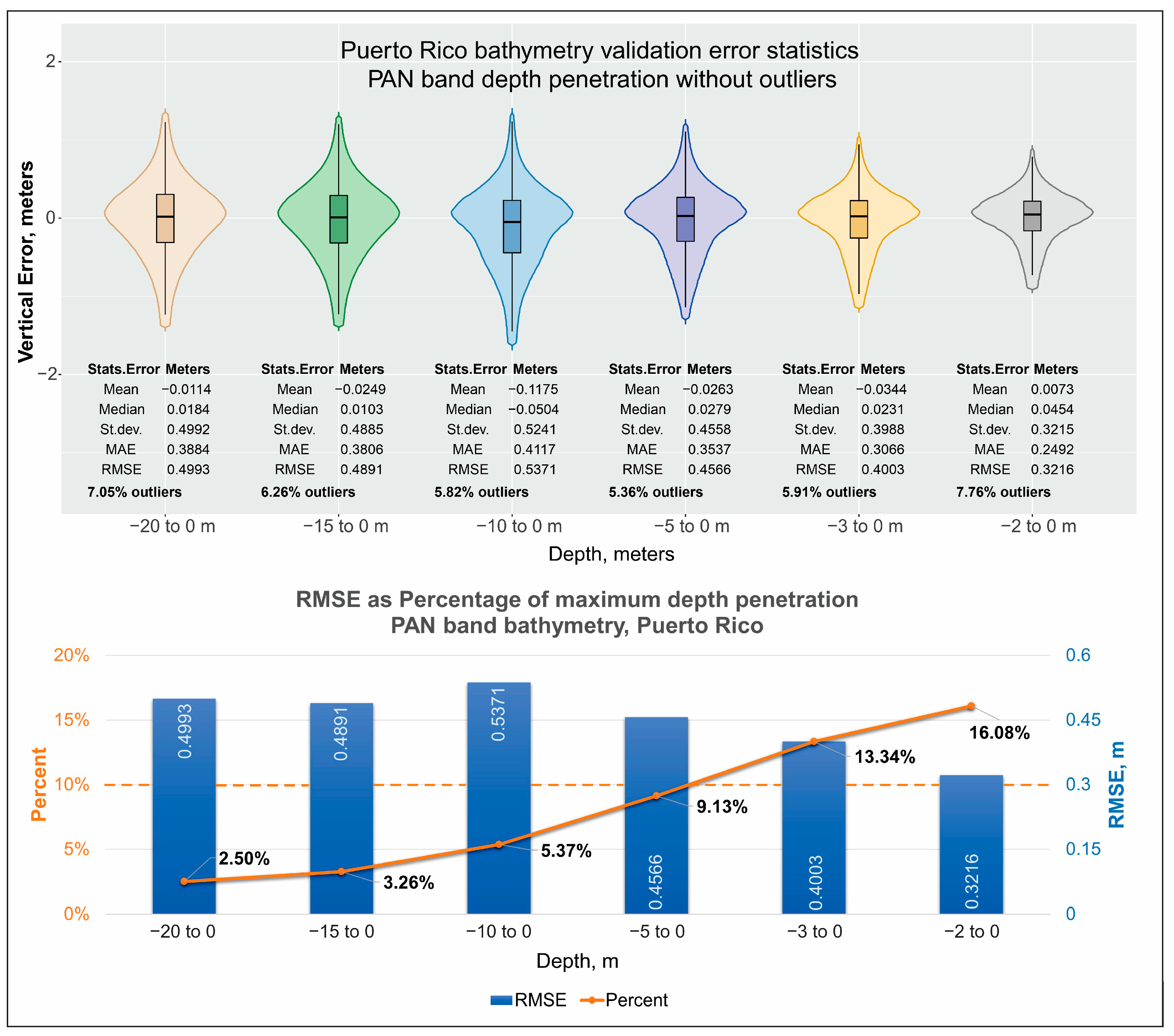
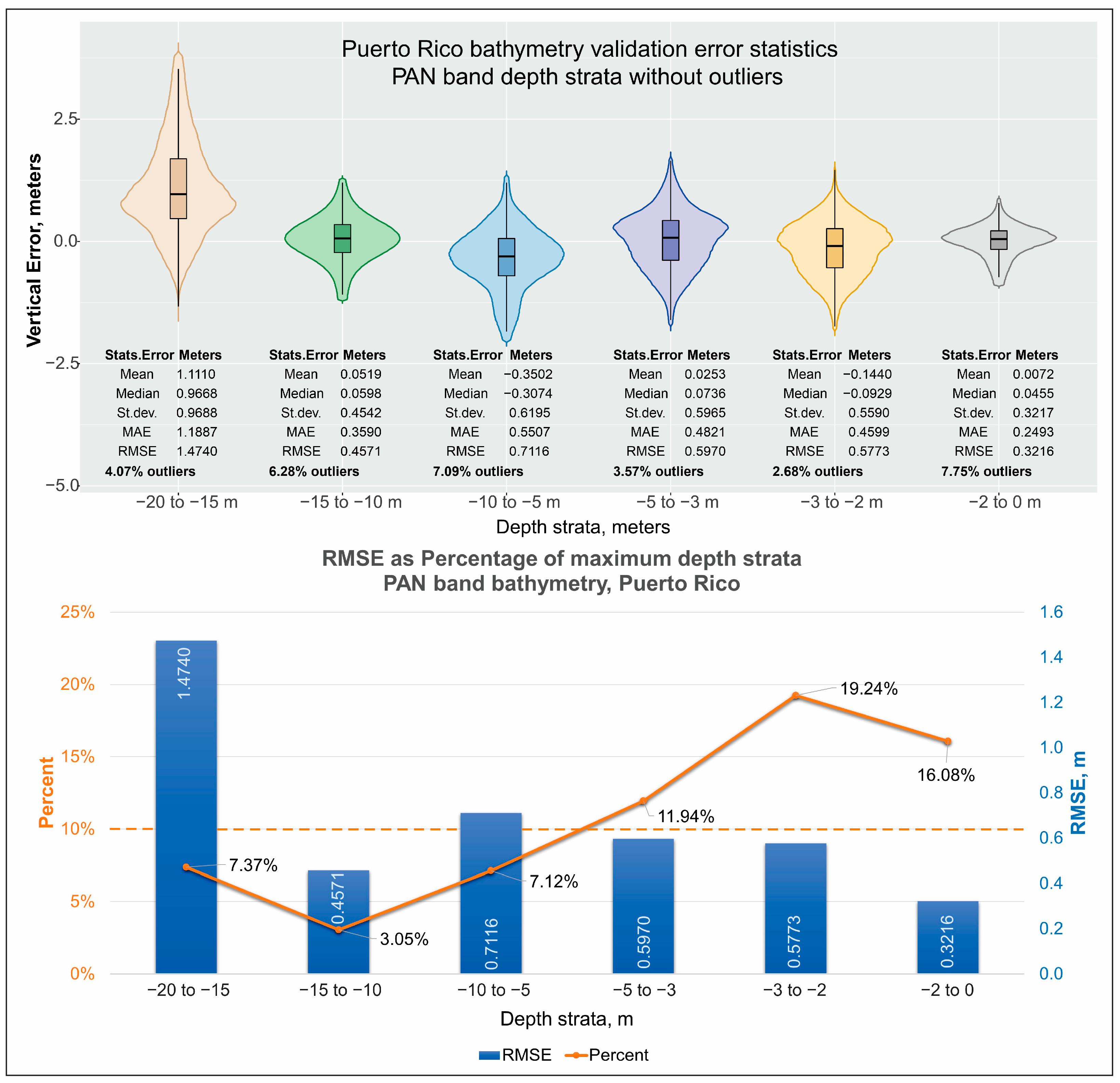
| Bathymetry validation error statistics by depth interval, PAN + GRN BA topography aligned | |||||||
| Statistics (meters) | 25–0 m | 20–0 m | 15–0 m | 10–0 m | 5–0 m | 3–0 m | 2–0 m |
| Mean | −0.4058 | −0.4099 | −0.3539 | −0.2345 | −0.0798 | −0.0621 | −0.0139 |
| Median | −0.3482 | −0.3513 | −0.2893 | −0.1547 | −0.0042 | 0.0096 | 0.0356 |
| St.dev. | 0.7836 | 0.7799 | 0.7353 | 0.6654 | 0.5243 | 0.4346 | 0.3484 |
| MAE | 0.6875 | 0.6862 | 0.6323 | 0.54 | 0.4053 | 0.3319 | 0.2664 |
| RMSE | 0.8824 | 0.8811 | 0.816 | 0.7055 | 0.5303 | 0.439 | 0.3487 |
| Differences between GRN bathymetry and PAN + GRN bathymetry validation errors statistics | |||||||
| Statistics (meters) | 25–0 m | 20–0 m | 15–0 m | 10–0 m | 5–0 m | 3–0 m | 2–0 m |
| Mean | −0.1382 | −0.139 | −0.1548 | 0.0169 | 0.1199 | 0.1216 | 0.0821 |
| Median | −0.1941 | −0.1948 | −0.2165 | −0.0241 | 0.0754 | 0.0855 | 0.0652 |
| St.dev. | −0.0047 | −0.0054 | 0.0181 | 0.0456 | 0.0839 | 0.1168 | 0.1286 |
| MAE | 0.0789 | 0.0796 | 0.0997 | 0.0477 | 0.0809 | 0.1124 | 0.1176 |
| RMSE | 0.0677 | 0.0682 | 0.093 | 0.0381 | 0.0792 | 0.1156 | 0.1332 |
Disclaimer/Publisher’s Note: The statements, opinions and data contained in all publications are solely those of the individual author(s) and contributor(s) and not of MDPI and/or the editor(s). MDPI and/or the editor(s) disclaim responsibility for any injury to people or property resulting from any ideas, methods, instructions or products referred to in the content. |
© 2023 by the authors. Licensee MDPI, Basel, Switzerland. This article is an open access article distributed under the terms and conditions of the Creative Commons Attribution (CC BY) license (https://creativecommons.org/licenses/by/4.0/).
Share and Cite
Palaseanu-Lovejoy, M.; Alexandrov, O.; Danielson, J.; Storlazzi, C. SaTSeaD: Satellite Triangulated Sea Depth Open-Source Bathymetry Module for NASA Ames Stereo Pipeline. Remote Sens. 2023, 15, 3950. https://doi.org/10.3390/rs15163950
Palaseanu-Lovejoy M, Alexandrov O, Danielson J, Storlazzi C. SaTSeaD: Satellite Triangulated Sea Depth Open-Source Bathymetry Module for NASA Ames Stereo Pipeline. Remote Sensing. 2023; 15(16):3950. https://doi.org/10.3390/rs15163950
Chicago/Turabian StylePalaseanu-Lovejoy, Monica, Oleg Alexandrov, Jeff Danielson, and Curt Storlazzi. 2023. "SaTSeaD: Satellite Triangulated Sea Depth Open-Source Bathymetry Module for NASA Ames Stereo Pipeline" Remote Sensing 15, no. 16: 3950. https://doi.org/10.3390/rs15163950