Article

Rainfall Erosivity in Peru: A New Gridded Dataset Based on GPM-IMERG and Comprehensive Assessment (2000–2020)

1
Servicio Nacional de Meteorología e Hidrología (SENAMHI), Lima 15072, Peru
2
Departamento de Física y Meteorología, Universidad Nacional Agraria La Molina (UNALM), Lima 15024, Peru
3
Géosciences Environnement Toulouse (GET), Université de Toulouse, CNRS, IRD, UPS, CNES, OMP, 31000 Toulouse, France
4
ISPA, Bordeaux Sciences Agro, INRAE, 33140 Villenave d’Ornon, France
*
Author to whom correspondence should be addressed.
Current address: Oeschger Centre for Climate Change Research and Institute of Geography, University of Bern, 3012 Bern, Switzerland.
Remote Sens. 2023, 15(22), 5432; https://doi.org/10.3390/rs15225432
Submission received: 1 August 2023 / Revised: 21 October 2023 / Accepted: 30 October 2023 / Published: 20 November 2023
(This article belongs to the Special Issue Remote Sensing of Water Resources Vulnerability)

Abstract

:
In soil erosion estimation models, the variables with the greatest impact are rainfall erosivity ( R E ), which is the measurement of precipitation energy and its potential capacity to cause erosion, and erosivity density ( E D ), which relates R E to precipitation. The R E requires high temporal resolution records for its estimation. However, due to the limited observed information and the increasing availability of rainfall estimates based on remote sensing, recent research has shown the usefulness of using observed-corrected satellite data for R E estimation. This study evaluates the performance of a new gridded dataset of R E and E D in Peru (PISCO_reed) by merging data from the IMERG v06 product, through a new calibration approach with hourly records of automatic weather stations, during the period of 2000–2020. By using this method, a correlation of 0.94 was found between PISCO_reed and R E obtained by the observed data. An average annual R E for Peru of 7840 MJ · mm · ha 1 · h 1 was estimated with a general increase towards the lowland Amazon regions, and high values were found on the North Pacific Coast area of Peru. The spatial identification of the most at risk areas of erosion was evaluated through a relationship between the E D and rainfall. Both erosivity datasets will allow us to expand our fundamental understanding and quantify soil erosion with greater precision.

1. Introduction

Soil erosion is one of the greatest environmental threats worldwide (Nearing et al. [1], Panagos et al. [2], Karlen et al. [3], Tripathi and Singh [4]), presenting multiple issues such as reduced crop yields, deterioration of water quality due to transport of fertilizers and pesticides, the decreased storage capacity of reservoirs due to sediment production, and losses in soils for cultivation [5,6,7]. There are various categories of erosion, such as water, wind, freezing, and mixed erosion, but the most frequent category with the highest proportion is water [8]. Water erosion of the soil damages the productive surface of the soil due to separation and transport processes, exposing the subsoil of the soil [9,10]. Therefore, the quality of the soil is affected by reducing its water retention capacity and amount of organic matter [11,12], endangering its various ecosystem services, such as CO 2 fixation, agricultural productivity, and flood risk reduction [13], which are expected to increase in demand due to urban expansion and changes in consumption patterns [14]. To prevent the worsening of soil erosion, it is necessary to apply public soil conservation policies based on the monitoring of regions susceptible to R E to understand and mitigate its effects, such as the reduction of agricultural productivity, food and water security, and the national economy [15,16,17,18].
The Intergovernmental Panel on Climate Change reports that there has been a continuous increase in CO 2 emissions in recent decades [19]. On average, the global concentration of CO 2 in the atmosphere increased by 40% from a preindustrial value in 2011. Evidence suggests that such an increase has resulted in an average increase in air temperature of 0.85 ° C (1880–2012), and according to the outputs of global climate models, it is predicted that by the end of the 21st century, the increase will reach 2 ° C with respect to the second half of the 19th century [19]. In this sense, it is expected that changes will occur in the hydrological cycle and, consequently, in the availability of water resources [19,20,21]. The change in the global water supply is expected to be ±10% with more intense storm events, depending on the region of analysis [19,22,23]. In Peru, some investigations on the impact of climate change converged toward a scenario with higher rainfall rates in the summer months (December–March), which would increase the erosive potential of storms, favoring soil loss from the available agricultural area, during these months [24]. Another consequence is the increase in the occurrence of events associated with soil loss, such as landslides [25,26]. For this reason, soil erosion in Peru should be part of the urgent national policy, aiming to identify and monitor areas more vulnerable to the loss of agricultural soils and promote actions to prevent, mitigate, or reverse its effects on desertification and soil degradation processes [27,28].
Soil erosion is caused by two physical processes: (i) separation of soil particles generated by the kinetic energy of the impact of raindrops and the (ii) transport of sediments by surface flow [1]. The level of erosion depends on the regional physiographic, soil, and precipitation characteristics [29], composed of two factors: the intensity of the precipitation and its kinetic energy at the surface of the soil [18]. One of the widely used indicators to quantitatively represent and measure the level of soil erosion, sheet and rill, is the multiannual index of RE [22,30,31,32] and erosivity density ( E D ), calculated as the ratio of R E and precipitation [33,34]. Generally, the R E is calculated in periods of less than 15 min, or adapted by means of statistical algorithms according to the available temporal resolution [35]. To predict soil erosion using R E , the empirical Revised Universal Soil Loss Equation (RUSLE) [34,36,37], which combines the influences of duration, magnitude, and intensity of storm events, can be used. Although the RUSLE method is estimated at the annual average level, it can also be calculated on shorter time scales to assess its variability [38]. In its formulation, the most dynamic and reactive factor to changes in climatic conditions is R E ; therefore, identifying temporal variability provides a more realistic and accurate assessment of soil erosion. For example, the seasonal estimate of R E is used to assess the risk of erosion in various vulnerable regions [11,39,40].
The classic R E equation requires precipitation time series from 1 to 15 min; unfortunately, this information is scarce globally [41,42]. However, through empirical equations, it is possible to use hourly or 30 min data. This convenient technique is commonly used in multiple regions [40,43]. More recently, a variety of research has examined the use of observed data and a satellite precipitation product (SPP) for R E estimation, with their respective limitations due to the source, data derivation model, and spatial scales [2,44,45]. Based on the above, the spatial estimation of R E can be grouped into three approaches: (i) observed-based R E : local estimates of weather stations and subsequent geospatial interpolation [44,46,47]; (ii) satellite-based R E : the use of satellite-based precipitation products (SPPs) [48,49,50]; and (iii) merged-based R E : a mix of both observed and simulated data sources, based on the correction of the R E obtained by the SPPs with respect to data from observed stations, at the national [8,18,51,52,53], regional [11,54], and global scales [40,52]. In this research, the merged-based R E method is used through seasonal satellite correction factors based on automatic weather stations (AWS) on a national scale. This procedure combines the advantages of AWS (accuracy at the hourly timescale) with that of the SPP (spatial variability), widely used as a complement in the analysis of various hydrological processes [55,56].
In South America, studies have been developed with the observed-based R E methodology for the estimation of the R E . In Brazil, Sanchez-Moreno et al. [57] used this method because they had more available information, obtaining an R E range of 1672 to 22,452 MJ · mm · ha 1 · h 1 with an increase from east to west; likewise, Mello et al. [58] identified areas in the northwest with very high R E (>20,000 MJ · mm · ha 1 · h 1 ) and in the northeast with medium R E rates (>2000 MJ · mm · ha 1 · h 1 ). Using merged-based R E , in Ecuador, Delgado et al. [59] estimated the R E based on observed stations, and the Integrated Multi-satellitE Retrievals for GPM (IMERG) obtained a national average of 3173 MJ · mm · ha 1 · h 1 . In Chile’s central region, Bonilla and Vidal [47] obtained an R E range of 50 to 6000 MJ · mm · ha 1 · h 1 with an increase from north to south. Moreover, Lobo and Bonilla [60] based on the hourly precipitation from AWS estimates the R E at a point level with a range of 68 to 3520 MJ · mm · ha 1 · h 1 . In addition, they highlighted that the use of rainfall at a higher temporal resolution results in a nonlinear decrease in the R E .
In Peru, there are investigations that use the three methods. Based on the observed-based R E approach, local studies such as that Romero et al. [61] in the north of the Andean region estimated an R E of 2950 MJ · mm · ha 1 · h 1 at a point level, while Mejía-Marcacuzco et al. [62] on the south coast in Tacna estimated an R E of 1190 MJ · mm · ha 1 · h 1 . Using the satellite-based R E method, some global studies determined an average R E in Peru of 2246 MJ · mm · ha 1 · h 1 [63]; on the other hand, through the Global Rainfall Erosivity Database (GloREDa) product developed by Panagos et al. [40], an R E range was estimated between 148 MJ · mm · ha 1 · h 1 in the Pacific Coast region and 14,226 MJ · mm · ha 1 · h 1 in the lowland Amazon. Using the merged-based R E technique, INRENA-Pura [64] prepared a map of soil erosion intensity at a national scale, which was published by the National Institute of Natural Resources (INRENA), using cartographic information, represented by national charts, aerial photographs, and images captured by radar and satellite. Additionally, Sabino Rojas et al. [65] developed a soil erosion atlas on an annual scale from 1981 to 2014, based on information from the PISCOp V1.0 product on a monthly scale. Aybar et al. [66] found a range from 0 to ±10,000 MJ · mm · ha 1 · h 1 . In summary, the R E present in Peru, including the aforementioned results, would be in the range of 0 to 15,000 MJ · mm · ha 1 · h 1 , with an average of 2000 to 3000 MJ · mm · ha 1 · h 1 , with lower values on the Pacific Coast, in contrast with the higher values in the high Andean and the Amazon regions. However, no references were found on the climatology and yearly and monthly evolution of the R E , as well as the properties of storm events, at a regional or local level, relevant information for sediment modeling and water erosion studies [67,68].
In this study, the PISCO_reed product was constructed through a seasonal calibration process based on AWS in order to (i) obtain a more accurate R E product on a national scale and (ii) perform a regional assessment of erosivity, which allows us to identify the areas most at risk from the negative effects of soil loss. For this reason, the specific objectives of this research are (a) realize a cross-validation of the R E database and (b) to evaluate spatiotemporal R E by estimating trends and identifying danger zones. Finally, this study has the utility of demonstrating the application of precipitation data based on satellite products and observed stations to estimate the R E at monthly, annual, and multiannual scales.

2. Study Area

Peru is located on the west coast of South America, between 0 ° 02N–17 ° 50.2S and 68 ° 10.2W–81 ° 90.2W, with an extension of 1285 million km 2 . This territory is characterized by high topographic variability, with an elevation range from sea level to 6685 meters above sea level (masl), with an average of 1489 masl. Peru exhibits high variability of various climatic factors, such as precipitation and temperature, as a result of the interaction of various influences and forcing features, such as atmospheric flow, the complex orography of the Andes, the cold Humboldt Current System, and El Niño Southern Oscillation [69,70,71,72].
In general, the average annual precipitation varies in the range of ±1 mm on the southern coast, while in the lowland Amazon, it reaches higher values of 4860 mm; the average is 1412 mm. The highest rainfall is in the month of February, and the minimum is during the month of July. In addition, in the Peruvian Andes, the climate is complex and is mainly controlled by the orography that acts as a topographic barrier to the flow of moisture, causing the formation of strong precipitation gradients on the eastern flanks of the Andes [66]. The inter-Andean valleys (≳500 mm) are mainly dominated by convective processes that channel moisture intrusions from the Amazon. At the same time, the influences of the cold and dry air masses coming from the Humboldt Current System cause the driest conditions on the Pacific Coast and on the western flanks of the Andes (≲500 mm). However, during the El Niño Southern Oscillation occurrence, the Humboldt Current System weakens, and the formation of severe convective storms can occur, especially over the North Pacific Coast [66].
For better clarity on the development and evaluation of R E in Peru, the study area was divided into different regions. This segmentation was based on (i) the classification of climatic sectors [73] and (ii) the availability of AWS (Figure 1); the regions were labeled as follows: North Pacific Coast (R1), Central and South Pacific Coast (R2), North Western Andes (R3), Central and South Western Andes (R4), North Eastern Andes (R5), Central and South Eastern Andes (R6), High Amazon (R7), Northern Low Amazon (R8), and Lowland Amazon Center and South (R9). These regions can be grouped into three zones: R1 and R2 (Pacific Coast); R3, R4, R5, and R6 (Andes); and R7, R8, and R9 (Amazon).

3. Materials and Methods

3.1. Overview

Stages, functions, and gridded/observed data used in this research are shown in the flowchart (Figure 2), obtaining as results the PISCO_reed product and its evaluation. First, the R E from the AWS and from IMERG was estimated on an hourly scale using the conventional RUSLE method. Then, the R E from satellite series was constructed through a correction based on the AWS, with a validation of the interpolation of the multiplicative factor by seasonal periods. Next, the uncertainty of the erosivity products generated was evaluated, taking the observed data as a reference. Second, the E D rates and the areas of greatest danger of erosivity were estimated. Moreover, trends of the annual R E series by region were calculated.

3.2. Data

The estimation and evaluation of the R E in Peru required gridded products and observed precipitation data: (i) SPP IMERG, (ii) AWS from SENAMHI, and (iii) Global R E gridded products. These datasets were used in this study to develop the methodology.

3.2.1. Satellite Rainfall

The increased accessibility to high spatiotemporal resolution SPPs, such as the Global Precipitation Measurement (GPM) mission, has facilitated the development of hydrological research. GPM, jointly developed by the National Aeronautics and Space Administration (NASA) and the Japan Aerospace Exploration Agency (JAXA), was put into orbit and has been in operation since 2014 as a successor to TRMM (deployed in 1997), to unite and increase precipitation estimates from a constellation of satellites [74]. NASA’s Goddard Earth Sciences Data and Information Services Center (GES DISC) provides access to GPM-derived products through multiple applications that contribute to knowledge about the water cycle and its impact from extreme natural events [45,75]. NASA’s Earth Observing System Data and Information System has defined three levels of products for the distribution and labeling of GPM products; level 3 is called IMERG. For precipitation estimation, IMERG is based on an algorithm that uses GPM microwave observations as a reference to combine, using various interpolation methods, such as CMORPH-KF [76], with multiple satellite data, such as passive microwave (PMW), geosynchronous infrared (IR), and TRMM microwave imager estimates (TMI), among others. Therefore, it presents advantages over TRMM in terms of temporal resolution (3 to 0.5 h), spatial resolution (0.25 ° to 0.1 ° ), and area covered (60 ° S–60 ° N). Furthermore, IMERG version 6 features two enhancements. The first is the length of the period covered by GPM, using TRMM estimates (2000–2014) to obtain hourly rainfall from June 2000 to the present [74]. The second is the distinction between liquid and non-liquid precipitation, to calculate the precipitation from this first ratio. IMERG classifies its products according to latency periods: Early, Late, and Final with ±4 h, ±14 h, and ±3.5 months, respectively [77]. The Early and Late versions only have a calibration for observed climatology, while the Final version uses the observed monthly rainfall from the Global Precipitation Climatology Center (GPCC) for bias correction. The GPM-IMERG-V06-Final product (IMERGF) contains the variable PrecipitationCal, calibrated precipitation with observed stations, expressed in m m / h . To estimate R E , this research uses IMERGF data from September 2000 to August 2020. The product is available in netCDF4 format, freely downloadable from the portal https://disc.gsfc.nasagov/datasets (accessed on 1 April 2023).

3.2.2. Observed Rainfall

The observed hourly precipitation used in this study was obtained from the National Hydrology and Meteorology Service of Peru (SENAMHI). The data were extracted from hourly rainfall at 322 AWS and 9 AWS with 10 min rainfall A W S _ 10 m i n located at altitudes ranging from 100 to 5000 masl, with an average of 2000 masl (Figure 1). The amount of AWS has increased in recent years, from 120 in 2014 to 320 in 2021. In addition, the temporal period of the seasons is from 1.5 to 6 years, with an average of 3.5 (Figure A1); therefore, this is the most extensive hourly dataset for the estimation of the R E in Peru. The analysis of the results derived from the AWS is classified in the nine climatic regions, obtaining a total of 180, 90, and 40 AWS in the Coast, Andes, and Amazon zones, respectively. SENAMHI provides this information with basic quality control (QC), with a procedure that can be divided into two stages: (i) filtering by extreme physical, national limits (401 mm/h) and internal consistency control and (ii) visual inspection of the hourly, daily, monthly, and annual series, to validate internal consistency and homogeneity. The reliability of the AWS data has been successfully tested in various investigations that evaluate the performance and accuracy of the SPPs in Peru [56].

3.2.3. Global R E Products

This study uses global R E products such as GloREDa and CMORPH for comparison purposes. GloREDa is based on observed data of high temporal resolution (1 to 60 min) that mainly cover the period from 2000 to 2020, collected from various countries of different regions and climates; however, in South America, the number of stations only represents 4% with an irregular geographic distribution [40,78]. The resulting global R E product has a spatial resolution of 0.01 ° and can be accessed through the European Soil Data Centre website (https://esdac.jrc.ec.europa.eu/, accessed on 30 August 2023).
On the other hand, CMORPH is a global precipitation satellite product, based on geostationary, low-orbit, and PMW satellites [18], with temporal resolution (30 min), spatial resolution (8 km × 8 km), temporal period (1998 to present), and coverage area (60 ° S–60 ° N), developed by the National Oceanic and Atmospheric Administration (NOAA) [79,80]. This product has been applied for the identification of extreme hydrological processes, such as R E ; Bezak et al. [52] obtained this variable at pixel level using the RUSLE method [81]. The RE from CMORPH was downloaded from https://esdac.jrc.ec.europa.eu/ (accessed on 30 January 2023).

3.3. Methodology

3.3.1. Gridded Product Construction

Estimation R E

The estimation of the R E requires a minimum period of 20 years of information in order to reduce the uncertainties and biases generated by dry and wet years [30]. Moreover, this indicator provide valuable information for storm event assessment separately; therefore, Wischmeier and Smith [30] recommend as storm event identification requirements (Figure 3) (i) the use of a time interval minimum (TMI) of 6 h between each event, (ii) hourly rainfall greater than 0.2 mm for hourly level and 0.1 mm for 30 min level, (iii) finally, the accumulated volume by each event being greater than 0.2 mm.
The precipitation intensity (I) for the hourly and sub-hourly scales was obtained through the relationship of the accumulated precipitation and its corresponding recording time (1):
I = P T
where I indicates the intensity of precipitation in m m / h , P is the precipitation in m m , and T is the recording time in hours. In each storm event, according to Wischmeier and Smith [30], the unit measure of kinetic energy ( e r ) is estimated at each chosen time resolution interval, Equation (2):
e r = 0.29 [ 1 0.72 × e x p ( 0.05 i r ) ]
where i r is the precipitation intensity during the time interval in m m / h . The sum of the unit kinetic energy, multiplied by the rainfall volume for each time interval in a storm event, results in its total kinetic energy E, expressed in the next Equation (3):
E = r = 1 m e r V r
where E is expressed in MJ · ha 1 and V r is the rainfall in mm, during an event. Subsequently, Brown and Foster [36] define R E ( E I 30 ) as the result of the multiplication of E with the maximum intensity in 30 min of each storm event, as indicated in Equation (4):
R E = E I 30 = E I 30 m a x
where E I 30 is expressed in MJ · mm · ha 1 · h 1 and I 30 is the maximum rainfall intensity by storm event in m m / h ; then R E is E I 30 grouped by year and is expressed as MJ · mm · ha 1 · h 1 · yr 1 . In the case of only having temporal resolutions of 60 min, Panagos et al. [53] and Yin et al. [11] suggest multiplying E× I 60 m a x with a correction coefficient ( C C 60 ); this value varies from 1.15 to 3.37 (Equation (5)):
R E = E I 30 = E × I 60 m a x × C C 60
where I 30 m a x corresponds to the maximum intensity of 30 min identified in each storm event. E I 30 is the equivalent to the R E of RUSLE, and C C 60 is the correction coefficient.
As part of the methodology, C C 60 was estimated by means of correlations between the R E obtained from A W S _ 10 m i n added to 30 min ( A W S _ 30 m i n ) and those obtained from a temporal resolution of 60 min ( A W S ); the distribution of both AWS is represented in Figure 1. Fischer et al. [82] identified an underestimation of the R E of RUSLE when using rainfall series with a temporal resolution greater than 30 min.

Estimation E D

The R E needs to be evaluated with wide availability of hourly rainfall; however, this information is scarce in Peru. To solve these deficiencies, Foster et al. [83] introduced the E D function. This erosivity index is more stable and independent of rainfall data availability than R E , since it depends on the number of erosive events [83]; moreover, it is used to evaluate erosion patterns [11]. Although the R E provides information on the erosive potential of rainfall, it does not provide information on the concentration of extreme storms during the year. On the other hand, the E D better represents the R E patterns and the type of precipitation during erosive events [84]. Very high E D values indicate high runoff, implying an area more prone to floods and intense storms [37,45,85]. The E D is the ratio of R E to precipitation [83], expressed through Equation (6):
E D = R E P
where the annual accumulated precipitation is measured in mm·yr 1 and the annual R E in MJ · mm · ha 1 · h 1 · yr 1 . The equation was applied on a monthly and annual scale. The estimation RE-IMERGF were evaluated through a pixel by pixel, while the RE-AWS was calculated by each station location; both results were classified by region.

Construction and Validation of R E

Various studies show a high correlation between the extreme rainfall (>99th) obtained from SPPs with rain gauge adjustment and observed stations in South America [66,86]; accordingly, their spatial distribution shows a good correlation with the R E estimate [38,51,87]. Therefore, there is evidence of using hourly rainfall from IMERGF to estimate RE-IMERGF, with respective correction-based RE-AWS. Correction of simulated data based on observed stations is widely used to improve the accuracy in the generation of multiple rainfalls datasets and their derived products [79,88,89].
Several studies identified a high correlation in the spatiotemporal variability between precipitation and R E [23,51,63]; therefore, the correction of RE-IMERGF was performed by rescaling precipitation with observed data, for each independent pixel, using an annual factor average by season. By extending the approach of Chen et al. [51], the correction process was as follows: (i) obtainment of the calibration factor by grouping the monthly series at the seasonal level (summer, autumn, winter, and spring) in the same period, 2015–2020; (ii) employ a linear regression between the point-gridded values from RE-AWS and RE-IMERGF in the four seasonal periods to obtain the slope of each linear model defined as the seasonal multiplicative factor (FME); (iii) spatial interpolation of the FME point values by using the inverse distance weighted interpolation (IDW) method, at the same native spatial resolution of IMERGF (0.1 ° ); (iv) spatial aggregation applied to reduce the spatial resolution from 0.1 ° to 0.25 ° , with the aim of avoiding spatial inconsistencies as a consequence of the high variability of the multiply factor; (v) and finally, PISCO_reed was obtained as a result of multiplying RE-IMERGF by the FME maps. The validation was realised at the pixel level with the observed data from RE-AWS during the common period, 2015–2020.

Metrics Validation

The performance of PISCO_reed was evaluated by regions with reference to RE-AWS, and both databases were compared by statistical correlation and magnitude difference. The statistical metrics were Pearson correlation coefficient (r) and the aggregation index (dr) [90]. The coefficient r is a measure of the relationship of strength between two variables where a result of 1 indicates a perfect relationship with a positive slope, while −1 indicates a relationship with a negative slope. The dr is similar to a correlation coefficient, except that it varies between −1 and 1, a high value (>0.5) indicating both high correlation and low absolute differences between the observed and simulated time series. In addition, due to the difference between the magnitudes of the hydrological variables in the study regions, it was necessary to have statistical metrics that indicate the relative difference between the observed and simulated data, through a normalization process. In the comparison of the samples, the relative differences are normalized by the observed sample. The normalized mean gross error (NMGE) and normalized mean bias (NMB) statistics were selected. NMGE is a measure of the mean relative deviation from the observed values and is independent of the magnitude of the hydrological variable, suitable for comparison between arid and humid regions. Meanwhile, NMB is useful for evaluating the R E of different monthly rates, since the mean bias is normalized by dividing it by the observed R E .

3.3.2. Erosivity Evaluation

Global and National Comparative Analysis

The performance of IMERGF for R E estimation and storm events properties, such as the intensity of precipitation, duration, accumulated precipitation, and number of events during 2015–2020, were evaluated using a statistical approach based on the results obtained by the AWS. In addition, a comparison was made in statistical terms by pixels between the observed data, PISCO_reed, and other global products that use the RUSLE method to estimate R E , such as the GloREDa product (2000–2020) developed by Panagos et al. [78] and the CMORPH R E product (1998–2020) obtained by Bezak et al. [52]. The temporal availability of global products is lightly different; therefore, it was contrasted by the multiyearly average of R E ; in the case of the correlation, a symmetric line with the origin at 0 was used as a reference.

Risk Map

In this study, we used E D to evaluate erosivity patterns and their effect under different ranges of rainfall, through a risk map [2]. Based on the combination of quartiles of the variables at a multiyear scale of E D and rainfall, we obtained 16 classes to characterize the susceptibility to soil erosivity, according to Das et al. [45]. In this range, areas with very high E D and very high to very low mean rainfall are the most vulnerable, while areas with very low E D , regardless of the precipitation rate, can be considered as those less prone to soil erosion, according to Panagos et al. [2].

4. Results

4.1. Spatiotemporal Distribution of R E and E D

In Figure 4, the properties of the storm events are compared, such as the average accumulated rainfall, maximum intensity, number storm, duration, annual rainfall, R E , and E D during the 2015–2020 period obtained from IMERGF and AWS. The RE-AWS correction was based on Equation (5) represented in Figure A2, where E I 30 is equal to RE-AWS based on the twenty one annual comparisons of R E identified in 9 A W S _ 30 m i n ; linear regression forced through the origin resulted in a slope ( C C 60 ) of 1.541 with a standard error of 0.01. Rainfall during the events and annual accumulated rainfall were slightly underestimated in parts of the Coast and Amazon zones. We noticed that in the Andes zone, there was a lower overestimation of the lowest daily rainfall and a high underestimation of the highest daily rainfall, a similar behavior found by Derin et al. [97]. On the contrary, the duration of the events was overestimated at the national level by IMERGF, at a ratio of up to 3 to 1 in the Andean regions. However, the greatest disagreement of magnitudes was found in the identification of the maximum intensities, with a high correlation by underestimation up to 5 times in all the regions, which has a more relevant impact on the estimation of the R E and E D . The maximum underestimations were found in the Amazon zone for R E and E D , reaching 6.2 and 8.3 times on average, respectively. In summary, this comparison showed good performance in correlation for storm properties since an SPP with higher temporal resolution is used, with a correlation greater than 0.74, except for the low value (0.47) found in the average duration of storms.
The precision of the annual R E estimates using IMERGF was also evaluated and compared with the AWS. The correlation coefficient of the mean annual RE-AWS and RE-IMERGF was 0.84. In general, taking AWS as a reference, the values based on IMERGF indicate an underestimation of the R E , present in all the analysis regions, with IMERGF values in R1 and maximum values in R7 and R9.
Based on the comparison of RE-IMERGF and RE-AWS at a seasonal scale for the period of 2015–2020, the multiplicative factors for each AWS were calculated (Figure 5). Values of less than 1 indicate an underestimation of IMERGF, while values greater than 1 indicate an overestimation. Figure 5 shows the variability between 0 and 28 in the histograms with a median of 5.5. There is a smaller amount of multiplicative factors < 1 (∼4% on average) that indicate the overestimation of the R E , mainly in the coastal regions during the winter and spring seasons. Meanwhile, the regions with the greatest underestimation of the R E are R3, R4, R5, R6, and R9, precisely where the most intense storm events are recorded. The interpolation of the multiplicative factors was added to reduce the spatial resolution to 0.4 ° , in order to reduce the factors with the greatest difference and proximity (Figure 5). Subsequently, IMERGF was corrected, through seasonal multiplication with the multiplicative factor map.
PISCO_reed from 2015–2020 was compared with the AWS data in Figure 6. The results show an improvement for dr with means in the range of 0.5 in R9 to 0.65 in R1. Additionally, the underestimation of the product is improved with means of NMB from −0.06 to −0.43. On the other hand, the NMGE medians range from 0.78 to 1.11, indicating an adequate performance of the R E from PISCO_reed, which will be analyzed by regional scale in the following sections. In addition, together with the E D product, both on a monthly and yearly scale, PISCO_reed was created.

4.1.1. Comparison with Global Products

When comparing the PISCO_reed product with the global products (GloREDa and CMORPH obtained from the multiyear average), taking as reference the observed data from the AWS (Figure 7 and Figure A1), a higher correlation was found in the PISCO_reed product (r = 0.94), finding slight over-estimations in some regions. On the other hand, the CMORPH product had a greater underestimation in all regions, mainly in R3, R4, R5, and R6. This underestimation was also observed in GloREDa, with the particularity of a marked overestimation of the R E in R1 and R2, where the R E was less than 3000 MJ · mm · ha 1 · h 1 .

4.1.2. National Analysis

Figure 8 shows the RE-AWS and the map of R E and E D from PISCO_reed. The R E and E D map is presented with a spatial resolution of 0.1 ° or ∼10 km. The mean R E value is 7118 MJ · mm · ha 1 · h 1 with a high variability that can be expressed by the standard deviation of 6231 MJ · mm · ha 1 · h 1 or a coefficient of variation of 0.88. The median R E is 7161 MJ · mm · ha 1 · h 1 , the first quartile is 841 MJ · mm · ha 1 · h 1 , and the third is 12,377 MJ · mm · ha 1 · h 1 . In the same way, the E D has an average value of 3.18 MJ · ha 1 · h 1 with a coefficient of variation of 0.62; in addition, the 25th, 50th, and 75th percentiles are 1.33, 3.48, and 4.49 MJ · ha 1 · h 1 , respectively.
The R E climatology map in Figure 9 shows that the month with the highest R E is March (954 MJ · mm · ha 1 · h 1 ), followed by December, January, and February (793 to 846 MJ · mm · ha 1 · h 1 ). The R E shows its lowest values for the period from June to September (224 to 397 MJ · mm · ha 1 · h 1 ), coinciding with the variability of precipitation climatologies, which have a high correlation in the range of 0.719 (March) to 0.923 (July). Likewise, the spatial distribution of the R E shows a notable difference between R5 and R9, with respect to the formerly R1 to R4, with high rates of R E in the first years.

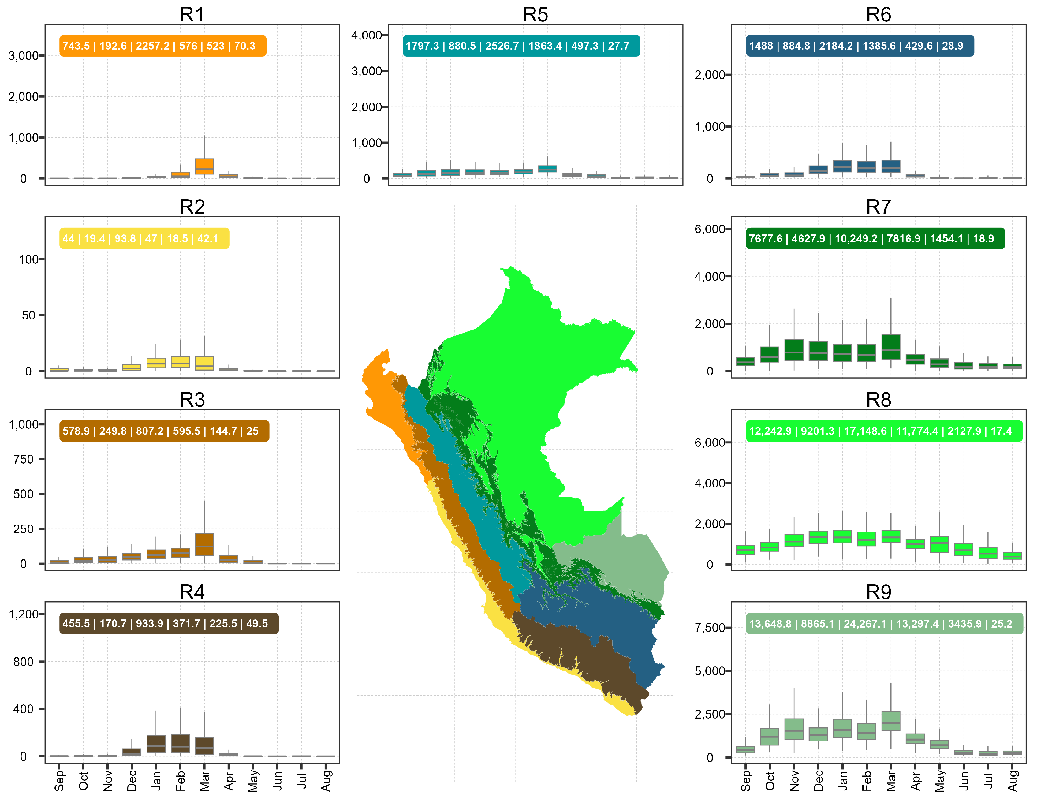
4.1.3. Regional Analysis

Figure A3 shows, at the regional level, the 2000–2020 annual variability of storm properties, such as total precipitation from erosive events, average storm duration, number of storm events, R E , and E D . In 2001, 2012, and 2017, when the R E reached its highest annual values, the total precipitation and the number and duration of storm events were also higher than in the other years. The mean annual duration of storm events is in the range of 3 and 10 h, the mean annual number of storms ranges from 40 to 280, the total precipitation ranges from 50 to 2500 mm, and the mean annual R E ranges from 40 to 11,000 MJ · mm · ha 1 · h 1 .
The properties of the average annual storm events are analyzed at the regional scale in Figure 10. The average number of storm events varies gradually from 47 in R2 to 242 in R8; that gradual scale in the regions is also shown in the average duration of the storms in the range of 2.5 to 8 h. The Amazon zone has a higher R E (7677 to 13,648 MJ · mm · ha 1 · h 1 ) compared with the coastal and Andean zones (44 to 1488 MJ · mm · ha 1 · h 1 ). This contrast is mainly due to the total precipitation, which on average is up to 13 times higher between the regions of the respective groups. In the same way, the analysis of the E D shows average rates of 0.5 to 2 MJ · ha 1 · h 1 in the coastal and Andean zones, while in the Amazon, the average E D varies from 3.8 MJ · ha 1 · h 1 in R7 to 5.6 MJ · ha 1 · h 1 in R9.
Figure 11 shows the monthly R E by region. The seasonality of the R E is visible in the regions, presenting the highest values of the R E during the wet season from December to April (average 510 MJ · mm · ha 1 · h 1 ), with maximum values in the month of March. Meanwhile, the low R E values are found during the dry season from June to September (average 152 MJ · mm · ha 1 · h 1 ), with minimum values during the months of July or August. Finally, a descriptive statistical summary is shown in Figure 11 and Figure A4.

4.2. Spatial Variation of Risk Areas

The spatial variation of the risk areas, classified into sixteen classes in Peru, is shown in Figure 12. High-risk areas for R E were mainly found in R8 and R9; only some areas were identified in R7 due to their high rates of precipitation and E D . These transition areas to the Amazon plain are associated with areas of high soil erosion and landslides, depending on the physiography. The rest of the regions (R3 to R7) belong to the medium precipitation classification but with high rates of E D associated with a medium risk of erosion. These regions are the ones that are frequently affected by soil erosion and landslides due to their physiography with steep slopes and intense rainfall. In the Andean zone, during the period of 2004–2013, there were 38 landslides registered with fatal consequences for the local population and high damage to the supply network at the national level [98]. In addition, the Andes mountains have multiple geological faults and anthropogenic soil erosion activities, and are affected by extreme hydrological events, such as El Niño.

4.3. RE Seasonal Trend

The spatial variation of seasonal trends (decadal) of R E , evaluated with a confidence level of 95% (p < 0.05), including the regional trend mean, is shown in Figure 13. The spring season shows only a punctual increase in the south of R8 with positive changes greater than 500 MJ · mm · ha 1 · h 1 by decade, while in the north of R8, the change is negative at rates of −800 MJ · mm · ha 1 · h 1 by decade. In the rest of the country, such as R1 to R4, there are no significant changes (∼150 MJ · mm · ha 1 · h 1 by decade) during all seasons. This same pattern is observed at R5 and R6 in the winter season; however, in the autumn and summer seasons, a slight increase is identified in these regions with trends of up to −250 MJ · mm · ha 1 · h 1 by decade. Finally, it is highlighted that R8 and R9 are the ones with the widest range of trends (−1700 to −900 MJ · mm · ha 1 · h 1 by decade), except during the winter season, where the variation is between −600 and −500 MJ · mm · ha 1 · h 1 by decade.

5. Discussion

5.1. Comparison with Other Studies and Analysis of Causes

Observed subdaily station data are a fundamental source of information on rainfall frequency and amount [8]. However, the scarce availability, irregular distribution, and spatial inconsistencies, in steep regions, limit the use of the observed rainfall [99]. Therefore, SPPs are an alternative solution to precipitation estimation, since they provide spatially continuous information over large geographic areas [100]. The complementary use of this information is already used in South America for the estimation of the R E with the RUSLE method on a monthly and annual scale [47,59]. The evaluation of the product obtained from R E in this study is compared with the hourly rainfall data, suitable for evaluating hydrological products based on hourly information, such as RE [45], which constitute the longest, most numerous hourly base and with quality control in Peru.
The main factors of uncertainty in the generation of the R E are the precision of precipitation data, the estimation model of the R E , and the correction factor in the conversion of time scales [8]. Furthermore, Catari et al. [101], identified the sources of the error in the estimation of the R E : erroneous measurements of precipitation, the efficiency of the kinetic energy equation of storms as a function of intensity, and the variation of spatial patterns.
This study is consistent with the R E obtained by Barurén [102]; however, the maximum average R E is higher than our product (41,106 MJ · mm · ha 1 · h 1 ). This may be due to the fact that the analysis periods are different, altering the final result of the multiyear product. In addition, Rosas and Gutierrez [103] agree with the quantification of erosion variability, finding an increase in erosion in the direction of R4 to R3, the latter region being the region with the highest erosion in the western Andes of Peru. In R2, the results are in the range obtained by Mejía-Marcacuzco et al. [62], with an analysis period within the years of this study of 1997–2020. In the South American region, one of the global R E products is GloREDa, which estimates this variable using globally observed data and the ERA5 precipitation reanalysis product; however, the largest differences between R E and GloREDa estimates were observed in South America due to underestimation of precipitation in mountainous regions, such as the Andes [52]. The observed stations used for the elaboration of this product are mainly from the Brazilian Amazon.

5.2. Limitations

The IMERGF presents strengths and weaknesses in the analysis of storm events in multiple regions around the world due to difference in rainfall intensities, stations used for correction, type of sensors, resolution temporal, etc. According to Derin et al. [104] and Manz et al. [97], IMERGF is better than other products, such as TMPA-V7, in terms of accuracy in estimating the frequency of occurrence and intensity of precipitation distribution in the Andean regions. Regarding the detection of daily rainfall volumes, Das et al. [45] reported that IMERGF is sensitive in identifying light and no rain conditions. Regarding the detection of extreme precipitation, the global average is satisfactory due to the correction of biases based on the observed stations [105]; therefore, for the geographical conditions of the Andean zone of Peru, Derin et al. [97] identified slight overestimations. These biases influence the underestimation of the R E in R1, R6, and R4, since IMERGF has limitations in detecting extreme storms. Therefore, seasonality from IMERGF precision undoubtedly resulted in seasonal variation in R E and E D biases.
IMERGF, being a high spatial resolution dataset, reduces the uncertainties in the spatial patterns caused by the interpolation of rainfall and its derivatives in geographical areas with low AWS density [45]. However, the scarcity of AWS in R8 limits the bias correction of the R E , although this region is more resilient to erosion due to its flat land cover and physiography. This region presents a lower level of danger in the generation of landslide events according to the map defined by Millán-Arancibia and Lavado-Casimiro [26].
The R E estimate is sensitive to the temporal resolution of the rainfall [45], which originally required 30 min for its calculation. Therefore, if we use a different temporal resolution, it is necessary to apply an appropriate regression function to obtain a result equivalent to the estimate of the R E . Various studies develop a correlation function based on 30 min resolutions in areas where subhourly rainfall is not available. Panagos et al. [2] found a high underestimation of the R E (∼56%) when using hourly rainfall without correction, but when using a correction factor, a good correlation was obtained. The use of an erroneous function, or a low and irregular distribution of rainfall stations for its development, can increase the bias of the estimate [45]. In this investigation, information from rainfall stations with 10 min temporal resolution was used for the first time to find an adequate correction factor for the hourly R E . We found a factor greater than 1.5, which indicates an underestimation of R E compared with the original calculation with 30 min records.

5.3. Applications

RE is a key factor in estimating soil erosion [23]. Rain and its kinetic energy are the main driver of soil water erosion processes. These processes are associated with the detachment of soil particles, the generation of runoff, and the triggering of mass movements [106,107]. On the other hand, agricultural practices without soil conservation measures together with the increase in the intensity of severe storms [23,108] would cause erosion and increase the amount of solids in suspension in rivers. This could clog reservoirs, raise riverbeds, and affect water quality, due to high turbidity levels in the rainy season.
High erosion rates have effects on the ground as well as effects external to it [11]. As a consequence, they are responsible for the contamination and low productivity of farmlands [109]. It is expected that the R E results developed in this research can be used to update the maps and identify regions vulnerable to this mode of erosion. We must understand the physical processes of soil erosion; for this reason, it is important to implement a monitoring system for erosion and sediment production in experimental basins. The results of this study can be considered in the planning of public policies to reduce erosion aimed at conserving soil productivity [110] and maintaining soil ecosystem services at a tolerable level [111], especially in regions where a large increase was detected.
In Peru, data from AWS are spatially scarce. Therefore, SENAMHI expects the installation of rain radars, which will make it possible to have high-resolution spatiotemporal information. This could potentially improve [112] estimates of R E [113].

6. Conclusions

In this research we generated PISCOp_reed V1.0, a new dataset in Peru for estimated and analyze by region the R E using the RUSLE methodology, based on a correction of IMERGF from the hourly and subhourly AWS for the period of 2000–2020. The following is concluded: through the spatial correction of RE-IMERGF based on the RE-AWS, it was possible to reduce the biases to analyze its spatial distribution at the national and regional levels, on various time scales (climatology, monthly, and annual). At national level, the R E mean was 7840 MJ · mm · ha 1 · h 1 , in the range of 0 to 60,000 MJ · mm · ha 1 · h 1 (R9), with a spatial distribution similar to rainfall. The results of this study indicate that the previous analyses underestimated the R E due to the underestimation of the maximum intensities by the use of daily rainfall data; however, the R E from PISCO_reed was in the range of regional studies in the Amazon and Pacific Coast zones, obtained with similar methodologies.
The PISCO_reed product has the advantage of quick and simple access to information for the characterization and identification of risk areas to erosion and trends by pixel level. A high risk of R E is indicated at the Amazon zone based on a combination of high rainfall and high E D , where the number of storms, R E , and E D are highest of all regions. In addition, the spatial analysis of risk areas suggests that it is insufficient to predict the R E only based on rainfall, especially in R1 and R4. This information provides a method and database for the implementation of soil conservation, management policies, water administration, disaster prevention, agricultural/forestry planning, and other applications for the management of hydrographic basins. Especially in the Andes and Amazon zones, there are significant changes in trends of R E in the last 20 years. At the national scale, we estimated that about 1.1% of all the pixels have statistically significant positive trends and 13.5% have statistically significant negative trends at the 95% confidence level.
In the coming years, through the use of radars for the identification of observed hourly precipitation, storm events will be able to be analyzed with greater precision, improving the accuracy of the PISCO_reed product.

Author Contributions

Conceptualization, L.G. and W.L.-C.; methodology, L.G., W.L.-C., A.H. and E.S.; software, L.G.; validation, L.G., A.H. and W.L.-C.; formal analysis, L.G. and W.L.-C.; investigation, L.G., A.H., E.S. and W.L.-C.; resources, W.L.-C. and L.B.; data curation, L.G., A.H. and E.S.; writing—original draft preparation, L.G.; writing—review and editing, L.G., A.H., E.S., L.B., F.F. and W.L.-C.; visualization, L.G. and A.H.; supervision, W.L.-C. and A.H.; project administration, W.L.-C.; funding acquisition, L.B. and F.F. All authors have read and agreed to the published version of the manuscript.

Funding

This research was funded by the National Hydrology and Meteorology Service (SENAMHI) of the Ministry of the Environment of Peru and the Research Institute for Development (IRD) of France.

Institutional Review Board Statement

Not applicable.

Informed Consent Statement

Informed consent was obtained from all subjects involved in the study.

Data Availability Statement

The PISCO_reed V1.0 product is openly available at https://doi.org/10.6084/m9.figshare.24416923 (accessed on 20 October 2023) in figshare [114] under GNU public license version 3.

Acknowledgments

The authors extend their appreciation to the anonymous reviewers for their thoughtful comments and valuable advice. In the data evaluation process, the statistical metrics of the OpenAir 2.8 package and the stats 4.0.2 package were used; for the processing of the climatology time series and grid products, the raster 4.1 package of the R 4.0.2 programming language was used.

Conflicts of Interest

The authors declare no conflict of interest.

Appendix A

Figure A1. Number of automatic weather stations with availability of information by year and mean during the period of 2014–2020.
Remotesensing 15 05432 g0a1
Figure A2. Relation between the annual rainfall erosivity (RE) from 60 min automatic weather station (AWS) and 60 and 30 min AWS for 2014–2019. Both REs expressed in MJ · mm · ha 1 · h 1 . The regression line is obtained from all these annual REs (21 points) and is forced through the origin. Additionally, the correlation Pearson (r) and the equation to estimate C C 60 are shown.
Remotesensing 15 05432 g0a2
Figure A3. Cross-validation of the correction factor from rainfall erosivity by IMERG and observed data by means of aggregation index (dr), normalized mean bias (NMB), and normalized mean gross error (NMGE).
Remotesensing 15 05432 g0a3
Figure A4. Map plot of PISCO_reed, GloREDa, and CMORPH rainfall erosivity (MJ · mm · ha 1 · h 1 ) based on observed data from weather automatic stations for 2015–2020.
Remotesensing 15 05432 g0a4
Figure A5. Characterization of storm events by year at the regional scale of precipitation (mm · d 1 ), number of storm events, average duration of storm events (h), and rainfall erosivity in MJ · mm · ha 1 · h 1 between results derived by pixels from IMERGF and AWS at the corresponding period in 2015–2020.
Remotesensing 15 05432 g0a5
Figure A6. Variation of rainfall erosivity (MJ · mm · ha 1 · h 1 ) by region at yearly and monthly scale.
Remotesensing 15 05432 g0a6

References

  1. Nearing, M.; Lane, L.; Lopes, V. Modelling Soil Erosion. In Soil Erosion Research Methods; Lal, R., Ed.; Soil and Water Conservation Society: Ankeny, IA, USA, 1994. [Google Scholar]
  2. Panagos, P.; Borrelli, P.; Poesen, J.; Ballabio, C.; Lugato, E.; Meusburger, K.; Montanarella, L.; Alewell, C. The new assessment of soil loss by water erosion in Europe. Environ. Sci. Policy 2015, 54, 438–447. [Google Scholar] [CrossRef]
  3. Karlen, D.L.; Ditzler, C.A.; Andrews, S.S. Soil quality: Why and how? Geoderma 2003, 114, 145–156. [Google Scholar] [CrossRef]
  4. Tripathi, R.; Singh, H. Soil Erosion and Conservation; Wiley Eastern Limited: Hoboken, NJ, USA, 1993. [Google Scholar]
  5. Sparovek, G.; Schnug, E. Temporal erosion-induced soil degradation and yield loss. Soil Sci. Soc. Am. J. 2001, 65, 1479–1486. [Google Scholar] [CrossRef]
  6. Pimentel, D. Soil erosion: A food and environmental threat. Environ. Dev. Sustain. 2006, 8, 119–137. [Google Scholar] [CrossRef]
  7. Lukić, T.; Lukić, A.; Basarin, B.; Ponjiger, T.M.; Blagojević, D.; Mesaroš, M.; Milanović, M.; Gavrilov, M.; Pavić, D.; Zorn, M.; et al. Rainfall erosivity and extreme precipitation in the Pannonian basin. Open Geosci. 2019, 11, 664–681. [Google Scholar] [CrossRef]
  8. Chen, Y.; Xu, M.; Wang, Z.; Gao, P.; Lai, C. Applicability of two satellite-based precipitation products for assessing rainfall erosivity in China. Sci. Total Environ. 2021, 757, 143975. [Google Scholar] [CrossRef]
  9. Jain, M.K.; Kothyari, U.C.; Raju, K.G. GIS based distributed model for soil erosion and rate of sediment outflow from catchments. J. Hydraul. Eng. 2005, 131, 755–769. [Google Scholar] [CrossRef]
  10. Lee, J.H.; Heo, J.H. Evaluation of estimation methods for rainfall erosivity based on annual precipitation in Korea. J. Hydrol. 2011, 409, 30–48. [Google Scholar] [CrossRef]
  11. Panagos, P.; Ballabio, C.; Borrelli, P.; Meusburger, K.; Klik, A.; Rousseva, S.; Tadić, M.P.; Michaelides, S.; Hrabalíková, M.; Olsen, P.; et al. Rainfall erosivity in Europe. Sci. Total Environ. 2015, 511, 801–814. [Google Scholar] [CrossRef]
  12. Pimentel, D.; Kounang, N. Ecology of soil erosion in ecosystems. Ecosystems 1998, 1, 416–426. [Google Scholar] [CrossRef]
  13. Diodato, N.; Bellocchi, G. Assessing and modelling changes in rainfall erosivity at different climate scales. Earth Surf. Process. Landforms 2009, 34, 969–980. [Google Scholar] [CrossRef]
  14. Tilman, D.; Fargione, J.; Wolff, B.; D’antonio, C.; Dobson, A.; Howarth, R.; Schindler, D.; Schlesinger, W.H.; Simberloff, D.; Swackhamer, D. Forecasting agriculturally driven global environmental change. Science 2001, 292, 281–284. [Google Scholar] [CrossRef] [PubMed]
  15. Schulze, K.; Alder, J.; Cramer, W.; Masui, T.; van Vuuren, D.; Ringler, C.; Alcamo, J. Changes in Nature’s Balance Sheet: Model-Based Estimates of Future Worldwide Ecosystem Services; Resilience Alliance: Decatur, GA, USA, 2005. [Google Scholar]
  16. Colombo, S.; Hanley, N.; Calatrava-Requena, J. Designing policy for reducing the off-farm effects of soil erosion using choice experiments. J. Agric. Econ. 2005, 56, 81–95. [Google Scholar] [CrossRef]
  17. Conner, W.H.; Day, J.W.; Baumann, R.H.; Randall, J.M. Influence of hurricanes on coastal ecosystems along the northern Gulf of Mexico. Wetl. Ecol. Manag. 1989, 1, 45–56. [Google Scholar] [CrossRef]
  18. Kim, J.; Han, H.; Kim, B.; Chen, H.; Lee, J.H. Use of a high-resolution-satellite-based precipitation product in mapping continental-scale rainfall erosivity: A case study of the United States. Catena 2020, 193, 104602. [Google Scholar] [CrossRef]
  19. Change, I.C. Climate Change 2013: The Physical Science Basis; Cambridge University Press: Cambridge, UK; New York, NY, USA, 2013. [Google Scholar]
  20. Buytaert, W.; De Bièvre, B. Water for cities: The impact of climate change and demographic growth in the tropical Andes. Water Resour. Res. 2012, 48. [Google Scholar] [CrossRef]
  21. Vuille, M. Climate Change and Water Resources in the Tropical Andes; Sustainable Development Department, Inter-American Development Bank (IADB): Washington, DC, USA, 2013. [Google Scholar]
  22. Field, C.B.; Barros, V.; Stocker, T.F.; Dahe, Q. Managing the Risks of Extreme Events and Disasters to Advance Climate Change Adaptation: Special Report of the Intergovernmental Panel on Climate Change; Cambridge University Press: Cambridge, UK; New York, NY, USA, 2012. [Google Scholar]
  23. Micić Ponjiger, T.; Lukić, T.; Basarin, B.; Jokić, M.; Wilby, R.L.; Pavić, D.; Mesaroš, M.; Valjarević, A.; Milanović, M.M.; Morar, C. Detailed Analysis of Spatial–Temporal Variability of Rainfall Erosivity and Erosivity Density in the Central and Southern Pannonian Basin. Sustainability 2021, 13, 13355. [Google Scholar] [CrossRef]
  24. Almazroui, M.; Ashfaq, M.; Islam, M.N.; Rashid, I.U.; Kamil, S.; Abid, M.A.; O’Brien, E.; Ismail, M.; Reboita, M.S.; Sörensson, A.A.; et al. Assessment of CMIP6 performance and projected temperature and precipitation changes over South America. Earth Syst. Environ. 2021, 5, 155–183. [Google Scholar] [CrossRef]
  25. Instituto Nacional de Defensa Civil. Compendio Estadístico del INDECI 2019, en la Preparación, Respuesta y Rehabilitación de la GRD; Instituto Nacional de Defensa Civil-INDECI: Lima, Peru, 2019. [Google Scholar]
  26. Millán-Arancibia, C.; Lavado-Casimiro, W. Rainfall thresholds estimation for shallow landslides in Peru from gridded daily data. Nat. Hazards Earth Syst. Sci. Discuss. 2023, 23, 1191–1206. [Google Scholar] [CrossRef]
  27. Huerta, A.; Lavado, W. Atlas Zonas Áridas del Perú; Servicio Nacional de Meteorologia e Hidrologia del Peru: Lima, Peru, 2021; pp. 16–18. [Google Scholar]
  28. Ministerio del Ambiente. Climático, Cambio; Ministerio del Ambiente: Lima, Peru, 2009. [Google Scholar]
  29. Jayawardena, A.; Rezaur, R. Drop size distribution and kinetic energy load of rainstorms in Hong Kong. Hydrol. Process. 2000, 14, 1069–1082. [Google Scholar] [CrossRef]
  30. Wischmeier, W.; Smith, D. Predicting Rainfall Erosion Losses: A Guide to Conservation Planning; Department of Agriculture, Science and Education Administration: Washington, DC, USA, 1978; Volume 537. [Google Scholar]
  31. Panagos, P.; Ballabio, C.; Borrelli, P.; Meusburger, K. Spatio-temporal analysis of rainfall erosivity and erosivity density in Greece. Catena 2016, 137, 161–172. [Google Scholar] [CrossRef]
  32. Goovaerts, P. Using elevation to aid the geostatistical mapping of rainfall erosivity. Catena 1999, 34, 227–242. [Google Scholar] [CrossRef]
  33. Xu, Z.; Pan, B.; Han, M.; Zhu, J.; Tian, L. Spatial–temporal distribution of rainfall erosivity, erosivity density and correlation with El Niño–Southern Oscillation in the Huaihe River Basin, China. Ecol. Inform. 2019, 52, 14–25. [Google Scholar] [CrossRef]
  34. Renard, K.G.; Freimund, J.R. Using monthly precipitation data to estimate the R-factor in the revised USLE. J. Hydrol. 1994, 157, 287–306. [Google Scholar] [CrossRef]
  35. Zhang, W.B.; Xie, Y.; Liu, B.Y. Rainfall erosivity estimation using daily rainfall amounts. Sci. Geogr. Sin. Kexue 2002, 22, 711–716. [Google Scholar]
  36. Brown, L.; Foster, G. Storm erosivity using idealized intensity distributions. Trans. ASAE 1987, 30, 379–386. [Google Scholar] [CrossRef]
  37. Kinnell, P. Event soil loss, runoff and the Universal Soil Loss Equation family of models: A review. J. Hydrol. 2010, 385, 384–397. [Google Scholar] [CrossRef]
  38. Vrieling, A.; Hoedjes, J.C.; van der Velde, M. Towards large-scale monitoring of soil erosion in Africa: Accounting for the dynamics of rainfall erosivity. Glob. Planet. Chang. 2014, 115, 33–43. [Google Scholar] [CrossRef]
  39. Meusburger, K.; Steel, A.; Panagos, P.; Montanarella, L.; Alewell, C. Spatial and temporal variability of rainfall erosivity factor for Switzerland. Hydrol. Earth Syst. Sci. 2012, 16, 167–177. [Google Scholar] [CrossRef]
  40. Panagos, P.; Borrelli, P.; Meusburger, K.; Yu, B.; Klik, A.; Jae Lim, K.; Yang, J.E.; Ni, J.; Miao, C.; Chattopadhyay, N.; et al. Global rainfall erosivity assessment based on high-temporal resolution rainfall records. Sci. Rep. 2017, 7, 4175. [Google Scholar] [CrossRef]
  41. Williams, R.; Sheridan, J. Effect of rainfall measurement time and depth resolution on EI calculation. Trans. ASAE 1991, 34, 402–0406. [Google Scholar] [CrossRef]
  42. Angulo-Martínez, M.; Beguería, S. Estimating rainfall erosivity from daily precipitation records: A comparison among methods using data from the Ebro Basin (NE Spain). J. Hydrol. 2009, 379, 111–121. [Google Scholar] [CrossRef]
  43. Padulano, R.; Rianna, G.; Santini, M. Datasets and approaches for the estimation of rainfall erosivity over Italy: A comprehensive comparison study and a new method. J. Hydrol. Reg. Stud. 2021, 34, 100788. [Google Scholar] [CrossRef]
  44. Wang, Z.; Zhong, R.; Lai, C.; Chen, J. Evaluation of the GPM IMERG satellite-based precipitation products and the hydrological utility. Atmos. Res. 2017, 196, 151–163. [Google Scholar] [CrossRef]
  45. Das, S.; Jain, M.K.; Gupta, V. A step towards mapping rainfall erosivity for India using high-resolution GPM satellite rainfall products. Catena 2022, 212, 106067. [Google Scholar] [CrossRef]
  46. Agnese, C.; Bagarello, V.; Corrao, C.; d’Agostino, L.; d’Asaro, F. Influence of the rainfall measurement interval on the erosivity determinations in the Mediterranean area. J. Hydrol. 2006, 329, 39–48. [Google Scholar] [CrossRef]
  47. Bonilla, C.A.; Vidal, K.L. Rainfall erosivity in central Chile. J. Hydrol. 2011, 410, 126–133. [Google Scholar] [CrossRef]
  48. Chen, M.; Shi, W.; Xie, P.; Silva, V.B.; Kousky, V.E.; Wayne Higgins, R.; Janowiak, J.E. Assessing objective techniques for gauge-based analyses of global daily precipitation. J. Geophys. Res. Atmos. 2008, 113. [Google Scholar] [CrossRef]
  49. Yan, S.; Mingnong, F.; Hongzheng, Z.; Feng, G. Interpolation methods of China daily precipitation data. J. Appl. Meteorol. Sci. 2010, 21, 279–286. [Google Scholar]
  50. Tapiador, F.J.; Turk, F.J.; Petersen, W.; Hou, A.Y.; García-Ortega, E.; Machado, L.A.; Angelis, C.F.; Salio, P.; Kidd, C.; Huffman, G.J.; et al. Global precipitation measurement: Methods, datasets and applications. Atmos. Res. 2012, 104, 70–97. [Google Scholar] [CrossRef]
  51. Chen, Y.; Duan, X.; Ding, M.; Qi, W.; Wei, T.; Li, J.; Xie, Y. New gridded dataset of rainfall erosivity (1950–2020) on the Tibetan Plateau. Earth Syst. Sci. Data 2022, 14, 2681–2695. [Google Scholar] [CrossRef]
  52. Bezak, N.; Borrelli, P.; Panagos, P. Exploring the possible role of satellite-based rainfall data in estimating inter-and intra-annual global rainfall erosivity. Hydrol. Earth Syst. Sci. 2022, 26, 1907–1924. [Google Scholar] [CrossRef]
  53. Yin, S.; Xie, Y.; Nearing, M.; Wang, C. Estimation of rainfall erosivity using 5-to 60-minute fixed-interval rainfall data from China. Catena 2007, 70, 306–312. [Google Scholar] [CrossRef]
  54. Vrieling, A.; Sterk, G.; de Jong, S.M. Satellite-based estimation of rainfall erosivity for Africa. J. Hydrol. 2010, 395, 235–241. [Google Scholar] [CrossRef]
  55. Herrera, S.; Kotlarski, S.; Soares, P.M.; Cardoso, R.M.; Jaczewski, A.; Gutiérrez, J.M.; Maraun, D. Uncertainty in gridded precipitation products: Influence of station density, interpolation method and grid resolution. Int. J. Climatol. 2019, 39, 3717–3729. [Google Scholar] [CrossRef]
  56. Huerta, A.; Lavado-Casimiro, W.; Felipe-Obando, O. High-resolution gridded hourly precipitation dataset for Peru (PISCOp_h). Data Brief 2022, 45, 108570. [Google Scholar] [CrossRef]
  57. Sanchez-Moreno, J.F.; Mannaerts, C.M.; Jetten, V. Rainfall erosivity mapping for Santiago island, Cape Verde. Geoderma 2014, 217, 74–82. [Google Scholar] [CrossRef]
  58. Mello, C.D.; Viola, M.; Beskow, S.; Norton, L. Multivariate models for annual rainfall erosivity in Brazil. Geoderma 2013, 202, 88–102. [Google Scholar] [CrossRef]
  59. Delgado, D.; Sadaoui, M.; Ludwig, W.; Méndez, W. Spatio-temporal assessment of rainfall erosivity in Ecuador based on RUSLE using satellite-based high frequency GPM-IMERG precipitation data. Catena 2022, 219, 106597. [Google Scholar] [CrossRef]
  60. Lobo, G.P.; Bonilla, C.A. Effect of temporal resolution on rainfall erosivity estimates in zones of precipitation caused by frontal systems. Catena 2015, 135, 202–207. [Google Scholar] [CrossRef]
  61. Romero, C.C.; Baigorria, G.; Stroosnijder, L. Changes of erosive rainfall for El Niño and La Niña years in the northern Andean highlands of Peru. Springer Clim. Chang. 2007, 85, 343–356. [Google Scholar] [CrossRef]
  62. Mejía-Marcacuzco, J.; Pino-Vargas, E.; Guevara-Pérez, E.; Olivos-Alvites, V.; Condori-Ventura, M. Predicción espacial de la erosión del suelo en zonas áridas mediante teledetección. Estudio de caso: Quebrada del Diablo, Tacna, Perú. Rev. Ing. UC 2021, 28, 252–264. [Google Scholar] [CrossRef]
  63. Riquetti, N.B.; Mello, C.R.; Beskow, S.; Viola, M.R. Rainfall erosivity in South America: Current patterns and future perspectives. Sci. Total Environ. 2020, 724, 138315. [Google Scholar] [CrossRef]
  64. INRENA-Peru. Informe técnico del Estudio de Inventario y Evaluación de Andenes; Ministerio de Agricultura: Lima, Peru, 1996. [Google Scholar]
  65. Sabino Rojas, E.; Felipe-Obando, O.; Lavado-Casimiro, W. Atlas de Erosión de Suelos por Regiones Hidrológicas del Perú; Nota Técnica Nº 002 SENAMHI-DHI-2017; Servicio Nacional de Meteorologia e Hidrologia del Peru: Lima, Peru, 2017; pp. 23–24. [Google Scholar]
  66. Aybar, C.; Fernández, C.; Huerta, A.; Lavado, W.; Vega, F.; Felipe-Obando, O. Construction of a high-resolution gridded rainfall dataset for Peru from 1981 to the present day. Hydrol. Sci. J. 2020, 65, 770–785. [Google Scholar] [CrossRef]
  67. Panagos, P.; Borrelli, P.; Matthews, F.; Liakos, L.; Bezak, N.; Diodato, N.; Ballabio, C. Global rainfall erosivity projections for 2050 and 2070. J. Hydrol. 2022, 610, 127865. [Google Scholar] [CrossRef]
  68. Boix-Fayos, C.; Barberá, G.; López-Bermúdez, F.; Castillo, V. Effects of check dams, reforestation and land-use changes on river channel morphology: Case study of the Rogativa catchment (Murcia, Spain). Geomorphology 2007, 91, 103–123. [Google Scholar] [CrossRef]
  69. Garreaud, R. The Andes climate and weather. Adv. Geosci. 2009, 22, 3–11. [Google Scholar] [CrossRef]
  70. Lavado-Casimiro, W.; Espinoza, J.C. Impactos de El Niño y La Niña en las lluvias del Perú (1965-2007). Rev. Bras. De Meteorol. 2014, 29, 171–182. [Google Scholar] [CrossRef]
  71. Bourrel, L.; Rau, P.; Dewitte, B.; Labat, D.; Lavado, W.; Coutaud, A.; Vera, A.; Alvarado, A.; Ordoñez, J. Low-frequency modulation and trend of the relationship between ENSO and precipitation along the northern to centre Peruvian Pacific coast. Hydrol. Process. 2015, 29, 1252–1266. [Google Scholar] [CrossRef]
  72. Rau, P.; Bourrel, L.; Labat, D.; Melo, P.; Dewitte, B.; Frappart, F.; Lavado, W.; Felipe, O. Regionalization of rainfall over the Peruvian Pacific slope and coast. Int. J. Climatol. 2017, 37, 143–158. [Google Scholar] [CrossRef]
  73. Cubas Saucedo, F. Sectorización Climática del Territorio Peruano; Nota Técnica N° 001-2020/SENAMHI/DMA/SPC (marzo 2020); Servicio Nacional de Meteorologia e Hidrologia del Peru: Lima, Peru, 2021; pp. 3–28. [Google Scholar]
  74. Huffman, G.J.; Bolvin, D.T.; Braithwaite, D.; Hsu, K.L.; Joyce, R.J.; Kidd, C.; Nelkin, E.J.; Sorooshian, S.; Stocker, E.F.; Tan, J.; et al. Integrated multi-satellite retrievals for the global precipitation measurement (GPM) mission (IMERG). In Satellite Precipitation Measurement Volume 1; Springer: Cham, Switzerland, 2020; pp. 343–353. [Google Scholar]
  75. Tan, J.; Huffman, G.J.; Bolvin, D.T.; Nelkin, E.J. IMERG V06: Changes to the morphing algorithm. J. Atmos. Ocean. Technol. 2019, 36, 2471–2482. [Google Scholar] [CrossRef]
  76. Huffman, G.; Bolvin, D.; Braithwaite, D.; Hsu, K.; Joyce, R.; Kidd, C.; Sorooshian, S.; Xie, P.; Yoo, S. The Day-1 GPM Combined Precipitation Algorithm: IMERG. In Proceedings of the AGU Fall Meeting Abstracts, San Francisco, CA, USA, 5–9 December 2011; Volume 2011, p. H41L-08. [Google Scholar]
  77. Huffman, G.J. The Transition in Multi-Satellite Products from TRMM to GPM (TMPA to IMERG). Algorithm Information Document. 2019. Available online: https://docserver.gesdisc.eosdis.nasa.gov/public/project/GPM/TMPA-to-IMERG_transition.pdf (accessed on 2 November 2021).
  78. Panagos, P.; Hengl, T.; Wheeler, I.; Marcinkowski, P.; Rukeza, M.B.; Yu, B.; Yang, J.E.; Miao, C.; Chattopadhyay, N.; Sadeghi, S.H.; et al. Global rainfall erosivity database (GloREDa) and monthly R-factor data at 1 km spatial resolution. Data Brief 2023, 50, 109482. [Google Scholar] [CrossRef]
  79. Xie, P.; Joyce, R.; Wu, S.; Yoo, S.H.; Yarosh, Y.; Sun, F.; Lin, R. Reprocessed, bias-corrected CMORPH global high-resolution precipitation estimates from 1998. J. Hydrometeorol. 2017, 18, 1617–1641. [Google Scholar] [CrossRef]
  80. Xie, P.; Joyce, R.; Wu, S.; Yoo, S.H.; Yarosh, Y.; Sun, F.; Lin, R. NOAA climate data record (CDR) of CPC morphing technique (CMORPH) high resolution global precipitation estimates. Version 2021, 1, w9va-q159. [Google Scholar]
  81. Renard, K.G. Predicting Soil Erosion by Water: A Guide to Conservation Planning with the Revised Universal Soil Loss Equation (RUSLE); US Department of Agriculture, Agricultural Research Service: Washington, DC, USA, 1997.
  82. Fischer, F.K.; Winterrath, T.; Auerswald, K. Temporal-and spatial-scale and positional effects on rain erosivity derived from point-scale and contiguous rain data. Hydrol. Earth Syst. Sci. 2018, 22, 6505–6518. [Google Scholar] [CrossRef]
  83. Foster, G.; Yoder, D.; Weesies, G.; McCool, D.; McGregor, K.; Bingner, R. User’s Guide—Revised Universal Soil Loss Equation Version 2 (RUSLE 2); USDA—Agricultural Research Service: Washington, DC, USA, 2002.
  84. Zhu, D.; Xiong, K.; Xiao, H. Multi-time scale variability of rainfall erosivity and erosivity density in the karst region of southern China, 1960–2017. Catena 2021, 197, 104977. [Google Scholar] [CrossRef]
  85. Dabney, S.M.; Yoder, D.C.; Vieira, D.A.N.; Bingner, R.L. Enhancing RUSLE to include runoff-driven phenomena. Hydrol. Process. 2011, 25, 1373–1390. [Google Scholar] [CrossRef]
  86. Palharini, R.S.A.; Vila, D.A.; Rodrigues, D.T.; Quispe, D.P.; Palharini, R.C.; de Siqueira, R.A.; de Sousa Afonso, J.M. Assessment of the extreme precipitation by satellite estimates over South America. Remote Sens. 2020, 12, 2085. [Google Scholar] [CrossRef]
  87. Fenta, A.A.; Tsunekawa, A.; Haregeweyn, N.; Yasuda, H.; Tsubo, M.; Borrelli, P.; Kawai, T.; Belay, A.S.; Ebabu, K.; Berihun, M.L.; et al. Improving satellite-based global rainfall erosivity estimates through merging with gauge data. J. Hydrol. 2023, 620, 129555. [Google Scholar] [CrossRef]
  88. Fick, S.E.; Hijmans, R.J. WorldClim 2: New 1-km spatial resolution climate surfaces for global land areas. Int. J. Climatol. 2017, 37, 4302–4315. [Google Scholar] [CrossRef]
  89. Cucchi, M.; Weedon, G.P.; Amici, A.; Bellouin, N.; Lange, S.; Müller Schmied, H.; Hersbach, H.; Buontempo, C. WFDE5: Bias-adjusted ERA5 reanalysis data for impact studies. Earth Syst. Sci. Data 2020, 12, 2097–2120. [Google Scholar] [CrossRef]
  90. Willmott, C.J.; Robeson, S.M.; Matsuura, K. A refined index of model performance. Int. J. Climatol. 2012, 32, 2088–2094. [Google Scholar] [CrossRef]
  91. Mann, H.B. Nonparametric tests against trend. Econom. J. Econom. Soc. 1945, 13, 245–259. [Google Scholar] [CrossRef]
  92. Kendall, M.G. Rank Correlation Methods; Charles Griffin: London, UK, 1948. [Google Scholar]
  93. Hirsch, R.; Scott, A.G.; Wyant, T. Investigation of Trends in Flooding in the Tug Fork Basin of Kentucky, Virginia, and West Virginia; Technical Report, US Geological Survey; Office of Surface Mining Reclamation and Enforcement and the U.S. Bureau of Mines: Washington, DC, USA, 1982.
  94. Ashraf, M.; Routray, J.L. Spatio-temporal characteristics of precipitation and drought in Balochistan Province, Pakistan. Nat. Hazards 2015, 77, 229–254. [Google Scholar] [CrossRef]
  95. Sen, P.K. Estimates of the regression coefficient based on Kendall’s tau. J. Am. Stat. Assoc. 1968, 63, 1379–1389. [Google Scholar] [CrossRef]
  96. Theil, H. A rank-invariant method of linear and polynomial regression analysis. In Henri Theil’s Contributions to Economics and Econometrics: Econometric Theory and Methodology; Springer: Berlin/Heidelberg, Germany, 1992; pp. 345–381. [Google Scholar]
  97. Derin, Y.; Anagnostou, E.; Berne, A.; Borga, M.; Boudevillain, B.; Buytaert, W.; Chang, C.H.; Chen, H.; Delrieu, G.; Hsu, Y.C.; et al. Evaluation of GPM-era global satellite precipitation products over multiple complex terrain regions. Remote Sens. 2019, 11, 2936. [Google Scholar] [CrossRef]
  98. Sepúlveda, S.A.; Petley, D.N. Regional trends and controlling factors of fatal landslides in Latin America and the Caribbean. Nat. Hazards Earth Syst. Sci. 2015, 15, 1821–1833. [Google Scholar] [CrossRef]
  99. Kühnlein, M.; Appelhans, T.; Thies, B.; Nauss, T. Improving the accuracy of rainfall rates from optical satellite sensors with machine learning—A random forests-based approach applied to MSG SEVIRI. Remote Sens. Environ. 2014, 141, 129–143. [Google Scholar] [CrossRef]
  100. Zhu, Q.; Chen, X.; Fan, Q.; Jin, H.; Li, J. A new procedure to estimate the rainfall erosivity factor based on Tropical Rainfall Measuring Mission (TRMM) data. Sci. China Technol. Sci. 2011, 54, 2437–2445. [Google Scholar] [CrossRef]
  101. Catari, G.; Latron, J.; Gallart, F. Assessing the sources of uncertainty associated with the calculation of rainfall kinetic energy and erosivity—Application to the Upper Llobregat Basin, NE Spain. Hydrol. Earth Syst. Sci. 2011, 15, 679–688. [Google Scholar] [CrossRef]
  102. Barurén, M.A.R. Cuantificación de la Erosión Hídrica en el Perú y los Costos Ambientales Asociados; Pontificia Universidad Catolica del Peru: Lima, Peru, 2016. [Google Scholar]
  103. Rosas, M.A.; Gutierrez, R.R. Assessing soil erosion risk at national scale in developing countries: The technical challenges, a proposed methodology, and a case history. Sci. Total Environ. 2020, 703, 135474. [Google Scholar] [CrossRef]
  104. Manz, B.; Páez-Bimos, S.; Horna, N.; Buytaert, W.; Ochoa-Tocachi, B.; Lavado-Casimiro, W.; Willems, B. Comparative ground validation of IMERG and TMPA at variable spatiotemporal scales in the tropical Andes. J. Hydrometeorol. 2017, 18, 2469–2489. [Google Scholar] [CrossRef]
  105. Ning, S.; Wang, J.; Jin, J.; Ishidaira, H. Assessment of the latest GPM-Era high-resolution satellite precipitation products by comparison with observation gauge data over the Chinese mainland. Water 2016, 8, 481. [Google Scholar] [CrossRef]
  106. Klik, A.; Haas, K.; Dvorackova, A.; Fuller, I.C. Spatial and temporal distribution of rainfall erosivity in New Zealand. Soil Res. 2015, 53, 815. [Google Scholar] [CrossRef]
  107. Nyssen, J.; Vandenreyken, H.; Poesen, J.; Moeyersons, J.; Deckers, J.; Haile, M.; Salles, C.; Govers, G. Rainfall erosivity and variability in the Northern Ethiopian Highlands. J. Hydrol. 2005, 311, 172–187. [Google Scholar] [CrossRef]
  108. Lenzi, M.; Di Luzio, M. Surface runoff, soil erosion and water quality modelling in the Alpone watershed using AGNPS integrated with a Geographic Information System. Eur. J. Agron. 1997, 6, 1–14. [Google Scholar] [CrossRef]
  109. Issaka, S.; Ashraf, M.A. Impact of soil erosion and degradation on water quality: A review. Geol. Ecol. Landscapes 2017, 1, 1–11. [Google Scholar] [CrossRef]
  110. Blanco-Canqui, H. Energy crops and their implications on soil and environment. Agron. J. 2010, 102, 403–419. [Google Scholar] [CrossRef]
  111. Grillakis, M.G.; Polykretis, C.; Alexakis, D.D. Past and projected climate change impacts on rainfall erosivity: Advancing our knowledge for the eastern Mediterranean island of Crete. Catena 2020, 193, 104625. [Google Scholar] [CrossRef]
  112. Auerswald, K.; Fischer, F.K.; Winterrath, T.; Brandhuber, R. Rain erosivity map for Germany derived from contiguous radar rain data. Hydrol. Earth Syst. Sci. 2019, 23, 1819–1832. [Google Scholar] [CrossRef]
  113. Kreklow, J.; Steinhoff-Knopp, B.; Friedrich, K.; Tetzlaff, B. Comparing Rainfall Erosivity Estimation Methods Using Weather Radar Data for the State of Hesse (Germany). Water 2020, 12, 1424. [Google Scholar] [CrossRef]
  114. Gutierrez, L. High-Resolution Gridded Rainfall Erosivity Dataset for Peru—PISCO_reed v1.0. 2023. Available online: https://figshare.com/articles/dataset/High-resolution_gridded_rainfall_erosivity_dataset_for_Peru_-_PISCO_reed_v1_0/24416923 (accessed on 20 October 2023).
Figure 1. Regions in the study area and locations of automatic weather stations (AWS) with subhourly or hourly rainfall data. Triangles represent 60 min AWS ( A W S _ 60 m i n ), blue crosses represent 10 min AWS ( A W S _ 10 m i n ), and circles represent the AWS for cross-validation ( A W S _ v a l i d a t i o n ).
Remotesensing 15 05432 g001
Figure 2. Rainfall erosivity analysis methodology.
Remotesensing 15 05432 g002
Figure 3. Example for storm event identification during February 2017 (month–day and hour format) at Alamor Automatic Weather Station in Piura. Blue spaces represent storm events, red line represents the minimum precipitation for identifying an event, 6 h is the time interval minimum between two events (TIM), and the minimum volume for an event is 0.2 mm.
Remotesensing 15 05432 g003
Figure 4. Seasonally based annual average regression line of (a) accumulated precipitation by storm event in mm, (b) maximum intensity mean by each storm event in mm·h 1 , (c) average number of storm events, (d) average duration of storm events in h, (e) accumulated annual rainfall yearly in mm, (f) rainfall erosivity in MJ · mm · ha 1 · h 1 , and (g) erosivity density in MJ · ha 1 · h 1 , between results derived by pixels from IMERGF and AWS at the same corresponding period in 2015–2020.
Remotesensing 15 05432 g004
Figure 5. (a) Map of the seasonal multiplier factor and the respective (b) histograms.
Remotesensing 15 05432 g005
Figure 6. Comparison of PISCO_reed and the observed rainfall erosivity. (a) Aggregation index, (b) normalized mean bias, and (c) normalized mean gross error.
Remotesensing 15 05432 g006
Figure 7. Comparison of rainfall erosivity (MJ · mm · ha 1 · h 1 ) from PISCO_reed, GloREDa, and CMORPH based on observed data for 2015–2020.
Remotesensing 15 05432 g007
Figure 8. (a) Rainfall Erosivity from the observed gauges and products by PISCO_reed: (b) rainfall erosivity (MJ · mm · ha 1 · h 1 ) and (c) erosivity density (MJ · ha 1 · h 1 ).
Remotesensing 15 05432 g008
Figure 9. Climatology (2000–2020) of rainfall erosivity (MJ · mm · ha 1 · h 1 ).
Remotesensing 15 05432 g009
Figure 10. Characterization of storm events by region (2000–2020): precipitation annual (mm), number storm, mean duration (h), rainfall erosivity (MJ · mm · ha 1 · h 1 ), and erosivity density (MJ · ha 1 · h 1 ).
Remotesensing 15 05432 g010
Figure 11. Climatology of rainfall erosivity (MJ · mm · ha 1 · h 1 ). Moreover, the multiannual stats are shown by region: mean, minimum, maximum, median, SD, CV.
Remotesensing 15 05432 g011
Figure 12. Risk map of erosivity in Peru as a function of rainfall (mm) and erosivity density (MJ · mm · ha 1 · h 1 ). The quartiles of these hydrological variables are presented in their table.
Remotesensing 15 05432 g012
Figure 13. Change of rainfall erosivity expressed as MJ · mm · ha 1 · h 1 per decade at 95% confidence level and the value of the mean trend by region is shown.
Remotesensing 15 05432 g013
Disclaimer/Publisher’s Note: The statements, opinions and data contained in all publications are solely those of the individual author(s) and contributor(s) and not of MDPI and/or the editor(s). MDPI and/or the editor(s) disclaim responsibility for any injury to people or property resulting from any ideas, methods, instructions or products referred to in the content.

