Article

TransHSI: A Hybrid CNN-Transformer Method for Disjoint Sample-Based Hyperspectral Image Classification

1
School of Surveying and Land Information Engineering, Henan Polytechnic University, Jiaozuo 454000, China
2
Key Laboratory of Mine Spatio-Temporal Information and Ecological Restoration, Henan Polytechnic University Ministry of Natural Resources, Jiaozuo 454000, China
*
Author to whom correspondence should be addressed.
Remote Sens. 2023, 15(22), 5331; https://doi.org/10.3390/rs15225331
Submission received: 13 September 2023 / Revised: 10 November 2023 / Accepted: 10 November 2023 / Published: 12 November 2023

Abstract

:
Hyperspectral images’ (HSIs) classification research has seen significant progress with the use of convolutional neural networks (CNNs) and Transformer blocks. However, these studies primarily incorporated Transformer blocks at the end of their network architectures. Due to significant differences between the spectral and spatial features in HSIs, the extraction of both global and local spectral–spatial features remains incomplete. To address this challenge, this paper introduces a novel method called TransHSI. This method incorporates a new spectral–spatial feature extraction module that leverages 3D CNNs to fuse Transformer to extract the local and global spectral features of HSIs, then combining 2D CNNs and Transformer to capture the local and global spatial features of HSIs comprehensively. Furthermore, a fusion module is proposed, which not only integrates the learned shallow and deep features of HSIs but also applies a semantic tokenizer to transform the fused features, enhancing the discriminative power of the features. This paper conducts experiments on three public datasets: Indian Pines, Pavia University, and Data Fusion Contest 2018. The training and test sets are selected based on a disjoint sampling strategy. We perform a comparative analysis with 11 traditional and advanced HSI classification algorithms. The experimental results demonstrate that the proposed method, TransHSI algorithm, achieves the highest overall accuracies and kappa coefficients, indicating a competitive performance.

Graphical Abstract

1. Introduction

The classification of HSIs is a crucial task in Earth observation missions. HSIs capture hundreds of bands per pixel in the spectral dimension, providing a vast amount of spectral–spatial information with a high spectral resolution [1]. HSI classification has enormous potential for various high-precision Earth observation applications, such as land cover identification [2], precision agriculture [3,4], change detection [5,6], environmental monitoring [7,8], and resource exploration [9].

1.1. Literature Review

The early approaches to HSI classification primarily relied on methods based on spectral features. These methods involved taking the spectral information from HSIs as input features, extracting features using classifier models, and ultimately performing a classification. Commonly used classifier models include K-nearest neighbor (KNN) [10], support vector machine (SVM) [11], random forest (RF) [12], and others. However, HSI acquisition is often affected by environmental factors, resulting in various forms of noise during the imaging process. Furthermore, the obtained spectral features may contain redundant information. As a result, many of the current research methods aim to address these challenges by initially reducing the dimensionality of the data. Techniques such as principal component analysis (PCA) [13], singular value decomposition (SVD) [14], linear discriminant analysis (LDA) [15], and independent principal component analysis (ICA) [16] are commonly employed. To leverage the spectral–spatial information present in HSIs, researchers [17] have improved traditional classifier models. However, these manual HSI classification feature extraction methods require expert help and cannot represent a large amount of complex data.
In recent years, due to the powerful feature extraction and adaptive learning capabilities, deep learning techniques have been applied to HSI classification by many researchers. Table 1 lists some of the most recent state-of-the-art techniques, including CNNs, recurrent neural networks (RNNs), graph convolutional networks (GCNs), generative adversarial networks (GANs), and Transformer, and discusses their advantages and limitations.
As one of the mainstream backbone architectures, CNN demonstrates strong capabilities in extracting spatial structural information and local contextual information in HSIs through global parameter sharing and local connectivity. For instance, Hu et al. [18] used five convolutional layers for HSI classification. However, these approaches failed to sufficiently exploit the spatial features inherent to the data.
To better extract the spectral–spatial features of HSIs, researchers have introduced higher-dimensional convolutions. For example, Yang et al. [19] developed a two-branch network structure by combining 1D CNNs and 2D CNNs models. Chen et al. [20] introduced a method based on 3D CNNs combined with regularization to extract 3D features efficiently. Meanwhile, Zhong et al. [21] proposed a spectral–spatial residual network(SSRN) for HSI classification. This method leverages the information from the previous layer of features to supplement the latter layer of features, significantly improving the utilization rate of the features. Roy et al. [22] combined the characteristics of 3D CNNs and 2D CNNs to propose a hierarchical network structure. This method fully extracts spectral–spatial features, reduces computational complexity, and improves classification accuracy. Building upon the fusion of 2D CNNs and 3D CNNs, Firat et al. [36] incorporated deep separable convolution to reduce network parameters effectively.
Most of the methods outlined above are based on CNN backbones and their variants, but they are often insufficient to detect subtle differences between spectral dimensions. As the mainstream backbone architecture, CNNs have shown a solid ability to extract spatial structure and local context information from HSIs, effectively improving classification performance. However, CNNs also struggle to capture sequence properties, mainly medium- and long-term dependencies. Therefore, when there are numerous categories for classification and the spectral features are highly similar, the classification performance tends to degrade [34]. The self-attention mechanism [37,38] may be a better choice, as it is not limited by distance and can focus on more valuable information, contributing to a more comprehensive capture of global contextual relationships.
Therefore, to better extract the spectral–spatial features of HSIs, researchers have introduced attention mechanisms. For example, Mei et al. [39] introduced the spectral–spatial attention networks (SSAN), which employ attention-based RNNs to extract essential features from continuous spectra and use attention-based CNNs to focus on significant spatial correlations between neighboring pixels. However, in real HSI scenarios, a large number of hyperspectral samples (or pixels) are typically present, and RNNs are not suitable for parallel training, reducing the efficiency of HSI classification.
The Transformer network [35] has been proposed to solve natural image classification tasks from a sequence data perspective. For example, Dosovitskiy et al. [40] applied Transformer to image classification tasks and proposed the Vision Transformer (ViT) network. This network utilizes a multi-head self-attention (MHSA) mechanism to efficiently process and analyze sequential data, allowing for the extraction of global information. He et al. [33] directly used the Transformer networks for HSI classification and proposed HSI-BERT, which has a global receiving domain and good generalization ability but only uses linear projection and does not consider local spatial context information. Therefore, several scholars [41,42] have combined CNNs and Transformer structures to jointly extract information on HSIs and take advantage of both benefits. For instance, He et al. [43] introduced the spatial–spectral Transformer (SST) model, which extracted spatial features using a network structure similar to that of VGGNet. The model further integrated a dense connection-enabled Transformer to capture sequential spectral relationships. Moreover, a classification task was accomplished by utilizing the multilayer perceptron (MLP). Sun et al. [44] developed the SSFTT model, which uses convolutional layers to extract shallow spectral and spatial features of HSIs and then introduces a Gaussian-weighted feature tokenizer into the ViT model for feature transformation, obtaining deep semantic information. In the studies mentioned above that integrate Transformer structures, it is customary to append Transformer modules solely at the end of the network architecture. However, due to substantial disparities between the spectral and spatial features in HSIs, the extraction of global and local spectral–spatial features remains incomplete.
To fully exploit the combined potential, scholars have studied the strategy of integrating CNNs and Transformer blocks. For example, Zhong et al. [45] introduced the spectral spatial transformation network (SSTN), which separately merged 2D CNNs and 3D CNNs into the self-attention mechanism. They constructed spatial attention and spectral association modules to surpass the limitations of convolutional kernels. However, the SSTN fails to further integrate the extracted local and global spectral–spatial features, making it challenging to capture the crucial information of the targets. Li et al. [46] proposed Next-ViT, a new generation of Vision Transformer that uses the next hybrid strategy (NHS) to stack next convolutional blocks (NCBs) and next transformer blocks (NTBs) in an effective hybrid paradigm to better capture local and global information, thereby improving the performance of various downstream tasks. However, this method has a relatively large number of parameters.
With the emergence of deep learning methods, the classification accuracy for commonly used HSI datasets has reached nearly 100% [36,47]. However, many of the above methods suffer from a common issue: training and test sets are constructed using random sampling, with both training and test samples being drawn from the same image. The random selection of training samples overlaps neighboring test samples, leading to a relatively high correlation between them and overly optimistic classification results [48,49]. Recognizing this problem, researchers have proposed various separation sampling strategies to ensure the sampling of training and test sets from different regions [50,51]. For instance, Liang et al. [52] introduced a separate sampling strategy to control random sampling and minimize the overlap between training and test samples. Moreover, IEEE GRSS also provides disjoint training and test sets for HSI classification competitions.

1.2. Contribution

Inspired by these studies, we aim to leverage the advantages of the Transformer model based on the self-attention mechanism, that is, by capturing the spectral–spatial relationship of HSI sequences at a long distance and solving the problem of the limited ability of CNN methods to obtain deep semantic features. In this paper, considering the characteristics of HSI, Transformer Encode modules are introduced at both shallow and deep stages of spectral–spatial feature extraction in the network, enabling the comprehensive extraction of global and local spectral–spatial information in HSIs. A novel HSI classification method named TransHSI is proposed. The proposed method is introduced and evaluated using the disjoint training and test sets. The main contributions of this paper are summarized below:
(1)
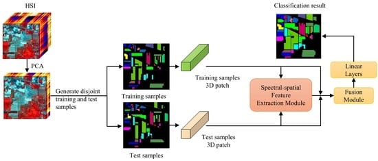
The TransHSI proposes a new spectral–spatial feature extraction module, in which the spectral feature extraction module combines 3D CNNs with different convolution kernel sizes and Transformer to extract the global and local spectral features of HSIs. In addition, the spatial feature extraction module combines 2D CNNs and Transformer to extract the global and local spatial features of HSIs. The module mentioned above thoroughly considers the disparities between spectral and spatial characteristics in HSIs, facilitating the comprehensive extraction of both the global and local spectral–spatial features in HSIs.
(2)
A fusion module is proposed, which first cascades the extracted spectral–spatial features and the original HSIs after dimensionality reduction and captures relevant features from different stages of the network. Secondly, a semantic tokenizer is used to transform the features to enhance the discriminant ability of features. Finally, the features are represented and learned in the Transformer Encode module to fully utilize the image’s shallow and deep features to achieve an efficient fusion classification of spectral–spatial features.
(3)
In this paper, the effectiveness of TransHSI is verified using three publicly available datasets, and competitive results are obtained. Crop classification is assessed using the Indian Pines dataset, and urban land cover classification is assessed using the Pavia University dataset and the Data Fusion Contest 2018. These results provide a reference for future research focused on HSI classification.
The remainder of this paper is organized as follows. Section 2 describes in detail the architecture of the proposed classification method. Section 3 presents the experimental datasets used to evaluate the performance of TransHSI and the experimental setup. Section 4 compares the classification performance of TransHSI with that of the other methods. Section 5 discusses the validity of TransHSI structures, feature visualization, and the impact of training set proportions on classification accuracy. Section 6 summarizes the paper and looks toward future work.

2. Materials and Methods

2.1. CNNs

In 1D CNNs, the convolutional kernels slide primarily along the spectral dimension to extract spectral features in HSIs. On 2D CNNs, the kernels move in both the height and width dimensions of the image to capture spatial features. In the case of 3D CNNs, the kernels slide in three directions: height, width, and spectral dimensions. When performing HSI classification tasks, this implies that using 3D CNNs allows for a more comprehensive utilization of the information embedded in HSIs. However, it is worth noting that 3D CNNs come with the largest parameter count, and to balance performance and computational complexity, this study employs both 2D CNNs and 3D CNNs to extract local features in the pixel spatial and spectral dimension. Within the neural network, the value v i , j α , β , γ at position ( α , β , γ ) on the j th feature cube in the i th layer can be represented using the following formula:
v i , j α , β , γ = g ( k h = 0 H i 1 w = 0 W i 1 r = 0 R i 1 ω i , j , k h , w , r v i 1 , k α + h , β + w , γ + r + b i , j )
where H i , W i , R i represent the width, height, and number of channels of the convolution kernel, respectively. ω i , j , k h , w , r is the weight parameter of position ( h , w , r ) connected to the k th feature cube, and b i , j is the bias. The function g ( · ) denotes the activation function.

2.2. Transformer Encode

The Transformer Encode module, shown in Figure 1b, comprises an MHSA layer, an MLP layer, two normalization layers, and two residual connection structures. The MHSA possesses the ability to capture long-range dependencies and adaptive spatial clustering. It comprises multiple self-attention layers stacked and integrated, enabling parallel computations and improving operational efficiency. Compared to a standard CNN, the Transformer Encode module incorporates advanced components such as layer normalization (LN) and the MLP. These components enhance the functionality and expressive power of the model. To learn multiple meanings, three learnable weight matrices W q , W k , W v are used to linearly map the flattened results, such as X f l a t 1 into a 3D invariant matrix comprising queries Q , keys K , and values V . The attention score is calculated using all Q and K , and the weight of the score is calculated using the softmax function. In summary, the self-attention layer is expressed as in the following formula.
Z = Attention ( Q , K , V ) = softmax ( Q K T d ) V
where Z represents the output from the attention layer and d represents the dimension of the keys K . Several different self-attention layers are combined into a single MHSA layer using Equation (2). The following formula expresses the MHSA layer.
MHSA = Concat ( Z 1 , Z 2 , , Z h ) W
where h is the head number of MHSA , h = 8 in this paper, W R h × d × t is the matrix parameter, and t is the number of tokens.
Following the MHSA and MLP layers, there is an LN layer and a residual connection, respectively. The role of the LN layer and the residual connection is to enhance the model’s stability, accelerate training convergence speed, and assist the network to better capture features and information. The MLP layer comprises two linear layers with a nonlinear activation function called the Gaussian Error Linear Unit (GELU) inserted between them. This activation function introduces the idea of random regularity in activation, thereby reducing gradient vanishing problems and enabling faster training.

2.3. Proposed Methodology

As shown in Figure 2, the classification method mainly includes three modules: the HSI pretreatment module, the spectral–spatial feature extraction module, and the fusion module, followed by classification through two linear layers. The spectral–spatial feature extraction module consists of a spectral feature extraction module and a spatial feature extraction module, both of which are composed of CNNs and Transformer components. This subsection of the paper provides a detailed description of the TransHSI method.

2.3.1. HSI Pretreatment Module

The original HSI data I R M × N × L are given, where M is the height, N is the width, and L is the number of spectral bands. Each pixel in I has L spectral bands, forming a single class vector Y = ( y 1 , y 2 , , y C ) R 1 × 1 × C , where C is the number of land cover categories. To reduce the spectral dimensions and computational complexity while eliminating redundant information, HSIs are processed using PCA. The HSI after dimensionality reduction is expressed as I p c a R M × N × B , where B is the number of spectral bands after PCA processing.
Then, 3D patches of the extraction of HSI data I p c a allow for the complete learning of spectral–spatial information around each pixel. The 3D patches X R S × S × B are created from Ipca, for which S × S represents the window size. The true label of each patch is determined by the label of the center pixel. A fill operation is performed on edge pixels when extracting a 3D patch around a single pixel. The width of the fill is ( S 1 ) / 2 . In each iteration of training, the order of the training dataset is randomly shuffled to ensure the diversity of training data, improve the generalization ability of the model, reduce the risk of overfitting, and increase the robustness of the model.

2.3.2. Spectral Feature Extraction Module

The spectral feature extraction module is shown in Figure 3a; the 3D patch X R S × S × B is initially processed through a 3D CNN with a kernel of 3 × 3 × 3 and a step size of 1. In this paper, to ensure that the size of the input and output data remains unchanged, padding is applied to the input data using padding = (kernel_size − 1)/2. The kernel_size represents the size of the convolutional kernel. Here, the 3D patch remains unchanged by utilizing the (1, 1, 1) padding strategy. The output of the 3D CNN is normalized using the batch normalization (BN) layer to obtain X 3 D 1 . Then, X 3 D 1 enters two 3D CNNs with a kernel of 5 × 3 × 3 and a kernel of 7 × 3 × 3 , and the output is X3D2. X 3 D 1 is connected with the X 3 D 2 residuals to obtain X 3 D 2 . The two 3D CNNs and residual connection structure are iterated again, and the result is X 3 D 2 . The utilization of multiple 3D CNNs is intended to thoroughly extract the local spectral information of 3D patches. The iteration result is input into a 2D CNN with a 1 × 1 kernel and 64 output channels to simplify the model and reduce the number of channels. Subsequently, the output of the 2D CNN is flattened into S 2 tokens. Finally, the tokens are input into the Transformer Encode module, and the output is denoted as X t r a n s 1 . The flattened result X f l a t 1 is connected with Xtrans1 residuals to obtain the output of the spectral feature extraction module, marked as X s p e . The Transformer Encode module enhances the learning of spectral band sequence properties, compensating for the underutilization of spectral information. The above process is expressed as in the following formulas.
X 3 D 1 = BN ( C o n v 3 D 1 ( X ) )
X 3 D 2 = C o n v 3 D 2 ( X 3 D 1 )
X 3 D 2 = X 3 D 1 + X 3 D 2
X f l a t 1 = Flatten ( C o n v 2 D 1 ( X 3 D 2 ) )
X t r a n s 1 = Trans ( X f l a t 1 )
X s p e = X f l a t 1 + X t r a n s 1
where C o n v 3 D denotes the 3D CNNs, C o n v 2 D denotes the 2D CNNs, Flatten ( · ) denotes flattening and Trans ( · ) denotes processing in the Transformer Encode module.
In the TransHSI network, there is a BN layer following the first 3D CNN, and after each subsequent convolutional layer, there is also a rectified linear unit (ReLU) layer and a dropout layer. The BN layer addresses the overfitting problem while speeding up network training and convergence. The ReLU layer adds nonlinearity to the model, thus improving its expressive power. The dropout layer enhances feature differentiation by increasing sparsity and helps to prevent overfitting. In this paper, the formula expression and illustration have been simplified, and the BN, ReLU, and dropout layers after the convolutional layer are not shown.

2.3.3. Spatial Feature Extraction Module

As shown in Figure 3b, the spatial feature extraction module initially employs 2D CNNs to capture local spatial information and subsequently utilizes the Transformer Encode module to learn long-range dependencies of pixels, effectively exploring the spatial information within HSIs. The module takes Xspe as the input and passes it through two 2D CNNs with 3 × 3 kernels, yielding an output denoted as X 2 D 2 . Next, similar to the two 3D CNNs in the spectral feature extraction module, the two 2D CNNs undergo residual connections and iterative processing before being fed into the spectral feature extraction module. The output of the spatial feature extraction module is recorded as X s p a . The spatial feature extraction module is represented as in the following formulas.
X 2 D 2 = C o n v 2 D 2 ( X s p e )
X 2 D 2 = X s p e + X 2 D 2
X f l a t 2 = Flatten ( X 2 D 2 )
X t r a n s 2 = Trans ( X f l a t 2 )
X s p a = X f l a t 2 + X t r a n s 2
where X 2 D 2 is the result of connecting the X2D2 and X s p e residuals, and X 2 D 2 is the result of iterating over two 2D CNNs and the residual connection structure.

2.3.4. Fusion Module

The fusion module is shown in Figure 4, which includes a cascade layer, a 2D CNN, a tokenizer module, and a Transformer Encode module.
The cascade layer plays a role in fusing the shallow and deep spectral–spatial features of HSIs. Specifically, it combines the original 3D patches X , the output Xspe of the spectral feature extraction module, and the output X s p a of the spatial feature extraction module. The fusion result is recorded as X c a t . To simultaneously learn fused feature results and reduce the number of channels, Xcat is subsequently fed into the 2D CNN with a kernel of 3 × 3 . Then, the output of the 2D CNN is flattened to obtain X i n R S 2 × D , where S represents the size of the 3D patch in the spatial dimension, either height or width. And D is the number of channels. The above process is expressed as in the following formulas:
X c a t = Concat ( X , X s p e , X s p a )
X i n = Flatten ( C o n v 2 D 3 ( X c a t ) )
To guide feature distribution regularization, the tokenizer operation uses two learnable weights initialized using the Xavier standard normal distribution, W a and W b , which are multiplied by X i n to extract critical features. That is, P feature vectors are selected from S 2 feature vectors for tokenization, where 0 < P < S 2 . The softmax function is employed to emphasize relatively significant information. This processing converts shallow and deep spectral–spatial features into tokenized semantic features, which aims to align the deep semantic features more closely with the distribution characteristics of the samples, thereby enhancing their separability [44]. The following equations summarize this process.
X a = softmax ( X i n W a ) T
X b = X i n W b
X o u t = X a X b
In this process, W a R D × P , W b R D × D ; X a R P × S 2 , X b R S 2 × D . X o u t R P × D is the output of the tokenizer. Xout consists of P tokens, which can be expressed as [ X 1 , X 2 , , X P ] .
To achieve a better HSI classification, a classification token X c l s is introduced here. It dynamically updates during network training, aggregating global features from other tokens to prevent bias towards any individual token. Then, the positional coding information X p o s is added. The above process is expressed in the following formula.
X t o k e n s = [ X c l s , X 1 , X 2 , , X P ] + X p o s
The positional encoding X p o s R ( P + 1 ) × D is a learnable parameter initialized using a normal distribution. As the network trains, it learns the row and column information of the pixels. X c l s possesses a fixed positional encoding (at position 0), alleviating interference caused by positional encoding. X t o k e n s R ( P + 1 ) × D is the output of the cascade X c l s and the addition of positional encoded information. Furthermore, the transformed features are passed through the Transformer Encode module to further learn the deep semantic features abstractly after fusion. Finally, the output is classified using two linear layers.

2.4. Implementation of TransHSI

As shown in Table 2, a detailed summary of the types of layers, output dimensions of maps, and the number of parameters for the TransHSI network is provided on the Pavia University dataset. The size of the 3D patch extracted using the Pavia University dataset is 15 × 9 × 9. In the spectral feature extraction module of the TransHSI network, 3D CNN_1 consists of 32@3×3×3 convolutional kernels; 3D CNN_2 and 3D CNN_4 each consist of 64@5×3×3 convolutional kernels, and 3D CNN_3 and 3D CNN_5 each consist of 32@7×3×3 convolutional kernels. In addition, 2D CNN_1 comprises 64@1×1 convolutional kernels. In the spatial feature extraction module, 2D CNN_2 and 2D CNN_4 each consist of 128@3×3 convolutional kernels, and 2D CNN_3 and 2D CNN_5 each consist of 64@3×3 convolutional kernels. Preceding the fusion module, the Transformer Encoder modules Trans_1 and Trans_2 outputs are resampled into 64@9×9 feature maps. Post fusion, 143(64 × 2 + 15) @9×9 feature maps are input into 2D CNN_6 containing 128@3×3 convolutional kernels. Subsequently, the 128@9×9 feature maps from 2D CNN_6 are resampled into 81 tokens of dimension 128. After selecting 5 feature vectors, which include 4 tokens and 1 introduced classifiable token, they are further processed through the Transformer Encoder module to output a 128 × 1 × 1 classifiable token. Finally, a linear layer generates a 9 × 1 × 1 prediction vector. In terms of the number of parameters, the total trainable parameters in the network amount to 1,049,569, with the highest number of parameters being attributed to 3D convolutions, followed by 2D convolutions.

3. Datasets and Experimental Setup

3.1. Experimental Datasets

In this study, three commonly used hyperspectral datasets are used for experiments: the Indian Pines dataset, the Pavia University dataset, and the Data Fusion Contest 2018. Moreover, the practice of randomly sampling training samples on the entire image is not adopted because in practical applications, the training and test samples are often collected from different locations. When the method uses the CNNs to process data, the receptive field will unconsciously contain the samples in the test set, meaning that the classification accuracy of the test set is set at a high level [1]. Therefore, experiments are performed using disjoint training and test sets. We downloaded the training sets for the Indian Pines and the Pavia University datasets are downloaded from the IEEE GRSS DASE website: http://dase.grss-ieee.org/, accessed on 6 October 2022. The training set for the Data Fusion Contest 2018 was manually selected. The number of training and test dataset samples for each class within the three datasets is shown in Table 3.

3.1.1. Indian Pines Dataset

The Indian Pines dataset was collected in northwestern Indiana, USA, using an Airborne Visible/Infrared Imaging Spectrometer (AVIRIS) sensor. It comprises two-thirds agriculture and one-third forest or other natural perennials. The HSI comprises 145 × 145 pixels, has a ground sampling distance (GSD) of 20 m, and 220 spectral bands that cover a wavelength range of 400–2500 nm. After removing the 20 noise and water absorption bands, 200 spectral bands were retained, namely 1–103, 109–149, and 164–219. This study primarily has 16 land cover categories, some of which are not mutually exclusive. The false-color map, ground truth map, and distribution of the training and test sets for the Indian Pines dataset are shown in Figure 5.

3.1.2. Pavia University Dataset

The Pavia University dataset is made up of scene data from the University of Pavia and its surroundings obtained using the Reflective Optics System Imaging Spectrometer (ROSIS) sensor. The sensor includes 103 spectral bands at 430–860 nm, and the image consists of 610 × 340 pixels with a GSD of 1.3 m. The scene contains nine land cover classes. The false-color map, ground truth map, and distribution of the training and test sets for the Pavia University dataset are shown in Figure 6.

3.1.3. Data Fusion Contest 2018 (DFC 2018)

The DFC 2018 was acquired with onboard sensors in downtown Houston, Texas, USA. The image consists of 610 × 2384 pixels, with a GSD of 1 m, which covers 48 adjacent bands of 380–1050 nm. The dataset includes not only urban categories, such as various types of buildings, roads, cars, and trains, but also various vegetation types, including healthy or stressed grass, deciduous or evergreen trees, etc. The dataset is part of the 2018 Data Fusion Contest, with 20 land cover categories. The false-color map, ground truth map, and distribution of the training and test sets for the DFC 2018 are shown in Figure 7.

3.2. Experimental Setup

In this paper, we used Python language and the PyTorch library to implement the classification method on the Windows 10 operating system. The experimental environment consists of the Intel(R) Core (TM) i9-9900K CPU @ 3.60 GHz, 32 GB memory, and NVIDIA GeForce RTX 2080 GPU. The learning rate is set to 0.001, and the batch size for both the training and test is set to 32. The experimental results are quantitatively evaluated using three indicators: overall accuracy (OA), average accuracy (AA), and the kappa coefficient ( κ ). The OA is the ratio of the total number of correctly classified samples to the total number of samples tested across all tests. AA is the average of the classification accuracy for all categories. The kappa coefficient is used to assess the categorical agreement of all classes and is calculated from the confusion matrix. If the sample size is the same for each category, OA and AA are equal. The strong difference between OA and AA may indicate a high percentage of specific categories being misclassified. The higher the value of the network on these three indicators, the better the classification ability of the network.
To fully utilize the spectral–spatial information of HSIs, as explained in Section 2.3.1, the original hyperspectral data undergo PCA processing. Then, 3D patches of a specific size around central pixels are selected as inputs for the network. The chosen size of a 3D patch significantly influences the amount of information utilized for classification and, to some extent, impacts the classification effect. As the patch size increases, more spectral–spatial information from the neighborhood may be introduced. However, a larger patch size can also introduce irrelevant information, leading to information redundancy and higher computational costs. Therefore, when determining the optimal patch size for each dataset, a balance must be struck between computational cost and classification performance. The number of spectral bands after PCA (denoted as B ) also follows a similar consideration. Due to significant differences in the sample sizes of the three datasets, we conducted experiments with different patch sizes and spectral band numbers, as illustrated in Figure 8 below. The OAs for the three datasets initially increased and then gradually decreased with an increase in input size. The change in OA was not consistent across datasets due to variations in data acquisition equipment and the spectral reflectance characteristics of ground objects. Specifically, for the Indian Pines dataset with a smaller sample size and a larger number of spectral bands (145 × 145 × 200), we used a patch size of 11 and B of 30. For the moderate-sized Pavia University dataset (610 × 340 × 103) and the DFC2018 with a larger sample size and fewer spectral bands (610 × 2384 × 48), we used a patch size of 9 and B of 15.

4. Experimental Result

This section uses several comparative experiments to verify the classification performance of the proposed method, TransHSI. The comparative methods include traditional classification methods like SVM [1] and RF [1]; CNN-based methods including 2D CNNs [20], 3D CNNs [20], HybirdSN [22], SSRN [21], and InternImage [53] based on deformable convolution (DCNv3); Transformer network-based methods such as ViT [40]; and methods combining CNNs and Transformer blocks, like Next-ViT [46], SSFTT [44], and SSTN [45]. To minimize experimental errors, each experiment was conducted three times, and the average of the three results was taken as the classification accuracy, as shown in Table 4, Table 5 and Table 6. In the TransHSI and comparative methods, the highest three comprehensive indicators are highlighted in bold.

4.1. Classification Results for the Indian Pines Dataset

As can be observed from Table 4, among all the classification methods applied to the Indian Pines dataset, the traditional classification method RF exhibits the poorest results in terms of the classification indicators OA, AA, and the kappa coefficient. At the same time, the classification accuracies of SVM are also low. In contrast, high-dimensional CNN methods such as 2D CNN, 3D CNN, and ViT networks with the MHSA mechanisms have better classification effects than traditional methods. This is because traditional classification methods rely solely on spectral information, whereas deep learning methods can also leverage spatial features [1]. Moreover, methods like HybirdSN, which mixes 2D CNNs and 3D CNNs, SSRN, which adds residual connection structures to 3D CNNs, InternImage based on DCNv3, and Next-ViT, SSFTT, and SSTN methods, which integrate CNNs and Transformer blocks, achieve classification accuracies higher than 81% with better classification effects. This implies that, compared to solely relying on convolution and attention mechanisms, hybrid networks have the capacity to learn and capture a broader range of spectral features and spatial contextual information [54]. The proposed TransHSI method achieved an OA of 87.75%, AA of 88.42%, and kappa coefficient of 86.11%, yielding the best performance. Among the six types of land cover categories, the TransHSI method achieves the highest accuracy. Additionally, the highly accurate classification methods HybirdSN and SSTN achieved OAs of over 84%. However, TransHSI outperformed HybirdSN and SSTN in terms of OA, with improvements of 1.96% and 3.28%, respectively. Regarding the AA, TransHSI demonstrated significant improvements compared to HybirdSN, SSFTT, and SSTN, with increases of 5.38%, 6.8%, and 20.4%, respectively. TransHSI also achieved a higher kappa coefficient than HybirdSN and SSTN, with improvements of 1.58% and 3.77%, respectively.
Figure 9 displays the classification results of the 12 methods in the Indian Pines dataset. It is evident that the TransHSI method (Figure 9l) exhibits the least noise, while SVM (Figure 9a) and RF (Figure 9b) suffer from significant noise scattering and a high number of misclassified areas, performing noticeably worse than the other classification networks. Additionally, in categories with less satisfactory visual results, the misclassification areas of the same land cover types, such as soybean-notill, soybean-mintill, and soybean-clean, are relatively smaller in the results of HybirdSN (Figure 9f), SSRN (Figure 9g), SSTN (Figure 9k), and TransHSI (Figure 9l). In the land cover category “corn-notill”, TransHSI has the fewest misclassified regions compared to the other three methods (Figure 9f,g,k). These observations align with the results presented in Table 4.

4.2. Classification Results for the Pavia University Dataset

As shown in Table 5 and Figure 10, the classification accuracies of SVM (Figure 10a) and RF (Figure 10b) for the Pavia University dataset are still very poor, with many misclassification areas in the visualization of the classification results. This is especially noticeable in the land cover categories of the “meadows” and “bare soil”, which are somewhat similar. However, this situation improved in the subsequent methods (Figure 10d–k). The TransHSI method (Figure 10l) demonstrates exemplary performance in the classification map. The proposed TransHSI method achieved an OA of 89.03%, AA of 91.34%, and kappa coefficient of 85.41%. In the TransHSI classification results, although the highest accuracy is achieved for a single land cover class, the OA and kappa coefficient metrics rank first among all the methods. The OAs of the SSRN, Next-ViT, InternImage, and SSFTT methods all reach more than 85%, but the OA of the TransHSI method is higher than those of the SSRN, Next-ViT, InternImage, and SSFTT methods by 0.92%, 1.71%, 2.51%, and 3.83%. The AA of the TransHSI method is second only to that of SSFTT. The kappa coefficient of the TransHSI method is 1.20%, 2.09%, 2.90%, and 4.63% higher than those of the SSRN, Next-ViT, InternImage, and SSFTT methods.

4.3. Classification Results for the DFC 2018

As can be seen from Table 6 and Figure 11, among all the classification methods applied to the DFC2018, the traditional classification method SVM has the lowest values in terms of the classification indicators OA, AA, and kappa coefficient. RF has higher values for these three comprehensive evaluation indicators than SVM, but its OAs do not reach 80%. From the visual classification in Figure 11, it is evident that SVM (Figure 11a) and RF (Figure 11b) have a more significant number of misclassified regions. In comparison with the ground truth map in Figure 6b, it can be observed that the classification map produced by the TransHSI method (Figure 11l) yields more accurate results. In the case of other methods, there is still salt-and-pepper noise present in the boundary regions of the “stadium seats”. The proposed TransHSI method achieves an OA of 86.36%, AA of 89.13%, and kappa coefficient of 82.53%. In the TransHSI classification results, although the accuracies of only five land cover categories reach the maximum values, both the OA and kappa coefficient indicators rank first among all networks. Secondly, the OAs of the SSRN, Next-ViT, and HybirdSN methods reach more than 85%, but their OAs are 0.72%, 0.84%, and 0.96% lower than that of the TransHSI method, respectively. The AA of the TransHSI method is second only to that of SSRN. The kappa coefficients of the SSRN, Next-ViT, and HybirdSN methods are lower than that of the TransHSI method by 0.93%, 1.13%, and 1.23%.

4.4. Visualization Analysis of TransHSI

As each method was subjected to three experiments on every dataset, the confusion matrices of the results were visualized by sorting them in ascending order of OAs and selecting the middle results. Figure 12 clearly illustrates that using TransHSI on all three datasets has led to the successful separation of the majority of the categories, as evidenced by the bar charts on the diagonal. However, some classes do not achieve ideal classification performance, such as “Corn” and “Buildings-Grass-Trees-Drives” on the Indian Pines dataset. Corn is often misclassified as “Soybean-clean”, possibly due to the scene being captured in June, where corn and soybean plants are in their early stages of growth, making them challenging to distinguish. Furthermore, as indicated in Table 4, the proposed method outperforms other comparative methods in terms of accuracy for “Buildings-Grass-Trees-Drives”, which consists of categories with diverse land cover types.
On the Pavia University dataset, “Gravel” is frequently misclassified as “Self-Blocking Bricks”. “Trees” and “Bare Soil” are commonly confused with “Meadows”. The false-color image of the Pavia University dataset indicates that these categories indeed share similarities, making them challenging to distinguish. Similarly, on the DFC 2018, “Roads”, “Sidewalks”, “Crosswalks”, “Major thoroughfares”, and “Highways” also exhibit mutual misclassifications due to their common road-related attributes, high similarity, and, thus, a tendency to be confused. Table 5 and Table 6 indicate that although the accuracy of most misclassified classes does not reach the highest values when compared to the other methods, their performance remains commendable.
The t-Distributed Stochastic Neighbor Embedding (t-SNE) [55] algorithm can map high-dimensional data to a lower-dimensional data, reducing the distances between similar categories, and increasing the gaps between different categories while preserving the local characteristics of the original data. To gain a more intuitive understanding of the feature learning process of the proposed method [56], we employed t-SNE to map the original sample and output layer features of three datasets into a two-dimensional space. As shown in Figure 13, the feature distribution of the original sample in the three datasets appears more chaotic, with higher levels of overlap, especially in datasets with a large number of categories like the Indian Pines dataset and DFC2018. Conversely, in the feature distribution of the output layer, the boundaries of most categories are clearly distinguished.

5. Discussion

TransHSI achieved competitive classification results on the Indian Pines, Pavia University, and DFC2018, indicating a certain degree of generalization capability of the proposed method. In this section, we will discuss the TransHSI network’s architecture and ablation experiment results on the Indian Pines and Pavia University datasets, analyzing the functionality of each network component. Additionally, on the three datasets, we will explore the impact of different training set percentages on the classification performance.

5.1. Ablation Experiments

5.1.1. Quantitative Comparison of Classification Results

This paper proposes a method of fusing convolution and Transformer models to extract the spectral–spatial features of hyperspectral data. To evaluate the effectiveness of each component of TransHSI, seven ablation experiments were conducted.The following is shown in Table 7.
The results of the TransHSI method and ablation experiments on the two hyperspectral datasets are shown in Table 8 and Table 9. From the tables, it is evident that TransHSI outperforms all other methods regarding both OA and the kappa coefficient. Furthermore, TransHSI achieves the highest AA on the Indian Pines dataset. On the Pavia University dataset, the AA of the TransHSI method is not much different from the highest AA. These indicate that the proposed network possesses a certain degree of robustness.
Specifically, in the Indian Pines and Pavia University datasets, we observed the following results from the ablation experiments: Method (a) exhibited the lowest accuracies, indicating that the spectral feature extraction module significantly influences the improvement in the classification performance. Methods (b) and (c) had minimal impacts on the classification results for the Indian Pines dataset, but they both had substantial impacts on the results for the Pavia University dataset, possibly due to differences in the dataset resolution. Method (c), unlike TransHSI, directly used learned features for classification, whereas TransHSI incorporated the features extracted in earlier stages. This suggests that the TransHSI network’s fusion of shallow and deep features effectively improves the classification accuracy. Method (d) removed all Transformer Encode modules, making it similar to the HybirdSN and SSRN methods, which primarily rely on CNN architectures. The classification accuracies of method (d) are higher than those of SSRN in the Indian Pines Dataset and slightly lower than those of HybirdSN. On the Pavia University Dataset, the classification accuracies of method (d) outperform those of HybirdSN but are slightly lower than those of SSRN. Its classification performance remains relatively stable across both datasets. In contrast, HybirdSN and SSRN achieved high accuracies on only one dataset each. Furthermore, when compared to the SSFTT and SSTN methods that combine CNN and Transformer modules, method (d) exhibits a slightly lower AA by approximately 1%, but a higher OA by about 1–6% and a higher kappa coefficient by 1–7%. This indicates that, in terms of overall correctly classified samples, method (d) holds a certain advantage over SSFTT and SSTN, which introduce long-range dependencies. However, deeper networks may not fully leverage their advantages if the specific characteristics of HSIs are not adequately considered. For example, when compared to Next-ViT (a method with a network depth of over 400 layers), method (d) still outperforms Next-ViT in all classification metrics on both datasets. Methods (e), (f), and (g), when compared to TransHSI, exhibited varying degrees of reduced accuracy. This suggests that integrating Transformer Encode modules into various components of the TransHSI network improved the extraction of global spectral–spatial information from HSIs, thereby enhancing the classification accuracy. Based on the analysis above, it is evident that each module in the TransHSI network plays a significant role in enhancing the HSI classification performances. Furthermore, it is worth noting that on the Pavia University dataset, methods (a), (f), and (g) achieve higher AA compared to TransHSI. This is because TransHSI performs less ideally in classifying the “Gravel” and “Bare Soil” categories, which are prone to misclassification. Additionally, the imbalance [57] in the sample categories in this dataset leads to TransHSI achieving the highest OA but a slightly lower AA.

5.1.2. Activation Maps Visualization

To further investigate the effectiveness of the TransHSI method and its ablation experiments, this paper conducted a qualitative experiment to visualize their activation maps. As shown in Figure 14, we used two different samples from the Pavia University dataset as inputs to compare the partial activation maps before the final Transformer Encode module. The red portion in the upper-left corner of sample 1 represents buildings, while the green portion in the lower-right corner represents trees. Sample 2 predominantly consists of painted metal sheets. In these two samples, this study observed that the activation maps of TransHSI (Figure 14a,e) exhibited a relatively uniform distribution of brighter areas, with high activation values in specific regions consistent with the targets (e.g., green trees in sample 1). In contrast, the activation maps from the ablation experiments (Figure 14b–d,f–h) displayed a more dispersed and chaotic distribution of high-activation-value areas, indicating a lower consistency with the targets. This is mainly attributed to the network structure of convolutional kernels [43]. When extracting spectral–spatial features, we introduced Transformer Encode modules separately, optimizing the extraction of global spectral–spatial features and key regions in HSIs. These feature visualization comparison results demonstrate that TransHSI can extract more effective spectral–spatial features.

5.2. Effect of Training Sample Percentages on Classification Results

We conducted experiments on three datasets with the Controlled Random Sampling Strategy [52], selecting different percentages of training samples for our proposed method, TransHSI, and algorithms based on CNNs and Transformer blocks. As shown in Figure 15, it is evident that as the training sample proportion increases, the classification accuracy of all methods improves. In comparison to TransHSI and Next-ViT, the classification performance of SSFTT and SSTN appears less satisfactory. This may be attributed to their failure to fully exploit the spectral–spatial information in HSI. The Next-ViT performs relatively poorly on the Indian Pines dataset when the training sample proportion is 5%, but it shows higher accuracy in other scenarios. Furthermore, in nearly all cases, TransHSI achieves the highest classification accuracy, even with a smaller number of samples, demonstrating the robustness of the proposed method.

6. Conclusions

This study developed a novel classification model called TransHSI. By integrating CNN and Transformer modules, we introduce a spectral–spatial feature extraction module designed to extract both global and local spectral and spatial information from HSIs. Additionally, the fusion module combines information from shallow and deep layers and introduces learnable parameters for feature transformation of flattened tokens, enhancing the features’ discriminative capacity. Through experiments conducted on three publicly available hyperspectral datasets with disjoint training and test sets, we carried out comprehensive comparisons with other recently proposed HSI classification methods. The results demonstrate that TransHSI excels, particularly on the Indian Pines, a low-resolution, small-sample dataset, where it achieves the best performance regarding OA, AA, and kappa coefficient. On the high-resolution, large-sample datasets, Pavia University and DFC2018, TransHSI still exhibits a competitive advantage, with AAs comparable to those of other leading methods and the highest OAs and kappa coefficients, showcasing comparable results to other methods. Furthermore, the ablation experiments and feature visualization results further validate the designed model’s effectiveness. In future research, we will optimize the network using lightweight module structures to reduce network complexity and enhance performance. Additionally, we will explore more neural network architectures and methods to further improve the accuracy and efficiency of HSI classification.

Author Contributions

All the authors made significant contributions to this work. Conceptualization, P.Z. and H.Y.; Methodology, P.Z. and H.Y.; Software, R.W.; Supervision, H.Y.; Validation, P.L.; Visualization, P.L.; Writing—Original Draft, P.Z.; Writing—Review and Editing, H.Y. and R.W. All authors have read and agreed to the published version of the manuscript.

Funding

This research was funded by National Natural Science Foundation of China (U1304402, 41977284) and Natural Science and Technology Project of Natural Resources Department of Henan Province (2019-378-16).

Data Availability Statement

The Indian Pines and the University of Pavia datasets are available online at http://dase.grss-ieee.org/, accessed on 6 October 2022. The Data Fusion Contest 2018 is available online at https://hyperspectral.ee.uh.edu/?page_id=1075, accessed on 10 October 2022. The source code for the TransHSI method is available at https://github.com/zpfx3/TransHSI, accessed on 6 March 2023.

Acknowledgments

The authors would like to thank the authors of all references used in this paper, the editors, and the anonymous reviewers for their detailed comments and suggestions.

Conflicts of Interest

The authors declare no conflict of interest.

References

  1. Audebert, N.; Le Saux, B.; Lefevre, S. Deep Learning for Classification of Hyperspectral Data: A Comparative Review. IEEE Geosci. Remote Sens. Mag. 2019, 7, 159–173. [Google Scholar] [CrossRef]
  2. Bhosle, K.; Musande, V. Evaluation of Deep Learning CNN Model for Land Use Land Cover Classification and Crop Identification Using Hyperspectral Remote Sensing Images. J. Indian Soc. Remote Sens. 2019, 47, 1949–1958. [Google Scholar] [CrossRef]
  3. Fong, A.; Shu, G.; McDonogh, B. Farm to Table: Applications for New Hyperspectral Imaging Technologies in Precision Agriculture, Food Quality and Safety. In Proceedings of the Conference on Lasers and Electro-Optics, Washington, DC, USA, 10–15 May 2020; p. AW3K.2. [Google Scholar]
  4. Lu, B.; Dao, P.D.; Liu, J.G.; He, Y.H.; Shang, J.L. Recent Advances of Hyperspectral Imaging Technology and Applications in Agriculture. Remote Sens. 2020, 12, 2659. [Google Scholar] [CrossRef]
  5. Wang, Q.; Yuan, Z.; Du, Q.; Li, X. GETNET: A General End-to-End 2-D CNN Framework for Hyperspectral Image Change Detection. IEEE Trans. Geosci. Remote Sens. 2019, 57, 3–13. [Google Scholar] [CrossRef]
  6. Zhan, T.; Song, B.; Sun, L.; Jia, X.; Wan, M.; Yang, G.; Wu, Z. TDSSC: A Three-Directions Spectral–Spatial Convolution Neural Network for Hyperspectral Image Change Detection. IEEE J. Sel. Top. Appl. Earth Obs. Remote Sens. 2021, 14, 377–388. [Google Scholar] [CrossRef]
  7. Zeng, D.; Zhang, S.; Chen, F.S.; Wang, Y.M. Multi-Scale CNN Based Garbage Detection of Airborne Hyperspectral Data. IEEE Access 2019, 7, 104514–104527. [Google Scholar] [CrossRef]
  8. Lowe, A.; Harrison, N.; French, A.P. Hyperspectral image analysis techniques for the detection and classification of the early onset of plant disease and stress. Plant Methods 2017, 13, 80. [Google Scholar] [CrossRef]
  9. Peyghambari, S.; Zhang, Y. Hyperspectral remote sensing in lithological mapping, mineral exploration, and environmental geology: An updated review. J. Appl. Remote Sens. 2021, 15, 031501. [Google Scholar] [CrossRef]
  10. Ma, L.; Crawford, M.M.; Tian, J. Local Manifold Learning-Based k-Nearest-Neighbor for Hyperspectral Image Classification. IEEE Trans. Geosci. Remote Sens. 2010, 48, 4099–4109. [Google Scholar] [CrossRef]
  11. Melgani, F.; Bruzzone, L. Classification of hyperspectral remote sensing images with support vector machines. IEEE Trans. Geosci. Remote Sens. 2004, 42, 1778–1790. [Google Scholar] [CrossRef]
  12. Kang, X.; Li, S.; Fang, L.; Li, M.; Benediktsson, J.A. Extended random walker-based classification of hyperspectral images. IEEE Trans. Geosci. Remote Sens. 2014, 53, 144–153. [Google Scholar] [CrossRef]
  13. Farrell, M.D.; Mersereau, R.M. On the impact of PCA dimension reduction for hyperspectral detection of difficult targets. IEEE Geosci. Remote Sens. Lett. 2005, 2, 192–195. [Google Scholar] [CrossRef]
  14. Menon, V.; Du, Q.; Fowler, J.E. Fast SVD With Random Hadamard Projection for Hyperspectral Dimensionality Reduction. IEEE Geosci. Remote Sens. Lett. 2016, 13, 1275–1279. [Google Scholar] [CrossRef]
  15. Jia, S.; Zhao, Q.; Zhuang, J.; Tang, D.; Long, Y.; Xu, M.; Zhou, J.; Li, Q. Flexible Gabor-Based Superpixel-Level Unsupervised LDA for Hyperspectral Image Classification. IEEE Trans. Geosci. Remote Sens. 2021, 59, 10394–10409. [Google Scholar] [CrossRef]
  16. Falco, N.; Benediktsson, J.A.; Bruzzone, L. A Study on the Effectiveness of Different Independent Component Analysis Algorithms for Hyperspectral Image Classification. IEEE J. Sel. Top. Appl. Earth Obs. Remote Sens. 2014, 7, 2183–2199. [Google Scholar] [CrossRef]
  17. Wang, Y.; Yu, W.; Fang, Z. Multiple Kernel-Based SVM Classification of Hyperspectral Images by Combining Spectral, Spatial, and Semantic Information. Remote Sens. 2020, 12, 120. [Google Scholar] [CrossRef]
  18. Hu, W.; Huang, Y.; Wei, L.; Zhang, F.; Li, H. Deep Convolutional Neural Networks for Hyperspectral Image Classification. J. Sens. 2015, 2015, 258619. [Google Scholar] [CrossRef]
  19. Yang, J.; Zhao, Y.-Q.; Chan, J.C.-W. Learning and Transferring Deep Joint Spectral–Spatial Features for Hyperspectral Classification. IEEE Trans. Geosci. Remote Sens. 2017, 55, 4729–4742. [Google Scholar] [CrossRef]
  20. Chen, Y.; Jiang, H.; Li, C.; Jia, X.; Ghamisi, P. Deep Feature Extraction and Classification of Hyperspectral Images Based on Convolutional Neural Networks. IEEE Trans. Geosci. Remote Sens. 2016, 54, 6232–6251. [Google Scholar] [CrossRef]
  21. Zhong, Z.; Li, J.; Luo, Z.; Chapman, M. Spectral–Spatial Residual Network for Hyperspectral Image Classification: A 3-D Deep Learning Framework. IEEE Trans. Geosci. Remote Sens. 2018, 56, 847–858. [Google Scholar] [CrossRef]
  22. Roy, S.K.; Krishna, G.; Dubey, S.R.; Chaudhuri, B.B. HybridSN: Exploring 3-D–2-D CNN Feature Hierarchy for Hyperspectral Image Classification. IEEE Geosci. Remote Sens. Lett. 2020, 17, 277–281. [Google Scholar] [CrossRef]
  23. Hang, R.L.; Liu, Q.S.; Hong, D.F.; Ghamisi, P. Cascaded Recurrent Neural Networks for Hyperspectral Image Classification. IEEE Trans. Geosci. Remote Sens. 2019, 57, 5384–5394. [Google Scholar] [CrossRef]
  24. Mou, L.C.; Ghamisi, P.; Zhu, X.X. Deep Recurrent Neural Networks for Hyperspectral Image Classification. IEEE Trans. Geosci. Remote Sens. 2017, 55, 3639–3655. [Google Scholar] [CrossRef]
  25. Hao, S.Y.; Wang, W.; Salzmann, M. Geometry-Aware Deep Recurrent Neural Networks for Hyperspectral Image Classification. IEEE Trans. Geosci. Remote Sens. 2021, 59, 2448–2460. [Google Scholar] [CrossRef]
  26. Ding, Y.; Zhang, Z.; Zhao, X.; Hong, D.; Cai, W.; Yu, C.; Yang, N.; Cai, W. Multi-feature fusion: Graph neural network and CNN combining for hyperspectral image classification. Neurocomputing 2022, 501, 246–257. [Google Scholar] [CrossRef]
  27. Hong, D.; Gao, L.; Yao, J.; Zhang, B.; Plaza, A.; Chanussot, J. Graph Convolutional Networks for Hyperspectral Image Classification. IEEE Trans. Geosci. Remote Sens. 2021, 59, 5966–5978. [Google Scholar] [CrossRef]
  28. Mou, L.; Lu, X.; Li, X.; Zhu, X.X. Nonlocal Graph Convolutional Networks for Hyperspectral Image Classification. IEEE Trans. Geosci. Remote Sens. 2020, 58, 8246–8257. [Google Scholar] [CrossRef]
  29. Wan, S.; Gong, C.; Zhong, P.; Du, B.; Zhang, L.; Yang, J. Multiscale Dynamic Graph Convolutional Network for Hyperspectral Image Classification. IEEE Trans. Geosci. Remote Sens. 2020, 58, 3162–3177. [Google Scholar] [CrossRef]
  30. Wang, J.; Guo, S.; Huang, R.; Li, L.; Zhang, X.; Jiao, L. Dual-Channel Capsule Generation Adversarial Network for Hyperspectral Image Classification. IEEE Trans. Geosci. Remote Sens. 2022, 60, 5501016. [Google Scholar] [CrossRef]
  31. Zhan, Y.; Hu, D.; Wang, Y.; Yu, X. Semisupervised Hyperspectral Image Classification Based on Generative Adversarial Networks. IEEE Geosci. Remote Sens. Lett. 2018, 15, 212–216. [Google Scholar] [CrossRef]
  32. Zhu, L.; Chen, Y.; Ghamisi, P.; Benediktsson, J.A. Generative Adversarial Networks for Hyperspectral Image Classification. IEEE Trans. Geosci. Remote Sens. 2018, 56, 5046–5063. [Google Scholar] [CrossRef]
  33. He, J.; Zhao, L.; Yang, H.; Zhang, M.; Li, W. HSI-BERT: Hyperspectral Image Classification Using the Bidirectional Encoder Representation from Transformers. IEEE Trans. Geosci. Remote Sens. 2020, 58, 165–178. [Google Scholar] [CrossRef]
  34. Hong, D.; Han, Z.; Yao, J.; Gao, L.; Zhang, B.; Plaza, A.; Chanussot, J. SpectralFormer: Rethinking Hyperspectral Image Classification with Transformers. IEEE Trans. Geosci. Remote Sens. 2022, 60, 5518615. [Google Scholar] [CrossRef]
  35. Vaswani, A.; Shazeer, N.; Parmar, N.; Uszkoreit, J.; Jones, L.; Gomez, A.N.; Kaiser, L.; Polosukhin, I. Attention Is All You Need. arXiv 2017, arXiv:1706.03762. [Google Scholar] [CrossRef]
  36. Fırat, H.; Asker, M.E.; Hanbay, D. Classification of hyperspectral remote sensing images using different dimension reduction methods with 3D/2D CNN. Remote Sens. Appl. Soc. Environ. 2022, 25, 100694. [Google Scholar] [CrossRef]
  37. Zhang, X.; Sun, G.; Jia, X.; Wu, L.; Zhang, A.; Ren, J.; Fu, H.; Yao, Y. Spectral-Spatial Self-Attention Networks for Hyperspectral Image Classification. IEEE Trans. Geosci. Remote Sens. 2022, 60, 5512115. [Google Scholar] [CrossRef]
  38. Ge, H.M.; Wang, L.G.; Liu, M.Q.; Zhu, Y.X.; Zhao, X.Y.; Pan, H.Z.; Liu, Y.Z. Two-Branch Convolutional Neural Network with Polarized Full Attention for Hyperspectral Image Classification. Remote Sens. 2023, 15, 848. [Google Scholar] [CrossRef]
  39. Sun, H.; Zheng, X.T.; Lu, X.Q.; Wu, S.Y. Spectral-Spatial Attention Network for Hyperspectral Image Classification. IEEE Trans. Geosci. Remote Sens. 2020, 58, 3232–3245. [Google Scholar] [CrossRef]
  40. Dosovitskiy, A.; Beyer, L.; Kolesnikov, A.; Weissenborn, D.; Zhai, X.; Unterthiner, T.; Dehghani, M.; Minderer, M.; Heigold, G.; Gelly, S.; et al. An Image is Worth 16x16 Words: Transformers for Image Recognition at Scale. arXiv 2020, arXiv:2010.11929. [Google Scholar] [CrossRef]
  41. Roy, S.K.; Deria, A.; Hong, D.; Rasti, B.; Plaza, A.; Chanussot, J. Multimodal Fusion Transformer for Remote Sensing Image Classification. arXiv 2022, arXiv:2203.16952. [Google Scholar] [CrossRef]
  42. Yang, L.; Yang, Y.; Yang, J.; Zhao, N.; Wu, L.; Wang, L.; Wang, T. FusionNet: A Convolution-Transformer Fusion Network for Hyperspectral Image Classification. Remote Sens. 2022, 14, 4066. [Google Scholar] [CrossRef]
  43. He, X.; Chen, Y.; Lin, Z. Spatial-Spectral Transformer for Hyperspectral Image Classification. Remote Sens. 2021, 13, 498. [Google Scholar] [CrossRef]
  44. Sun, L.; Zhao, G.; Zheng, Y.; Wu, Z. Spectral–Spatial Feature Tokenization Transformer for Hyperspectral Image Classification. IEEE Trans. Geosci. Remote Sens. 2022, 60, 5522214. [Google Scholar] [CrossRef]
  45. Zhong, Z.; Li, Y.; Ma, L.; Li, J.; Zheng, W.-S. Spectral–Spatial Transformer Network for Hyperspectral Image Classification: A Factorized Architecture Search Framework. IEEE Trans. Geosci. Remote Sens. 2022, 60, 5514715. [Google Scholar] [CrossRef]
  46. Li, J.; Xia, X.; Li, W.; Li, H.; Wang, X.; Xiao, X.; Wang, R.; Zheng, M.; Pan, X. Next-ViT: Next Generation Vision Transformer for Efficient Deployment in Realistic Industrial Scenarios. arXiv 2022, arXiv:2207.05501. [Google Scholar] [CrossRef]
  47. Firat, H.; Asker, M.E.; Bayindir, M.İ.; Hanbay, D. 3D residual spatial–spectral convolution network for hyperspectral remote sensing image classification. Neural Comput. Appl. 2022, 35, 4479–4497. [Google Scholar] [CrossRef]
  48. Ahmad, M.; Ghous, U.; Hong, D.; Khan, A.M.; Yao, J.; Wang, S.; Chanussot, J. A Disjoint Samples-Based 3D-CNN With Active Transfer Learning for Hyperspectral Image Classification. IEEE Trans. Geosci. Remote Sens. 2022, 60, 5539616. [Google Scholar] [CrossRef]
  49. Zhang, F.; Yan, M.; Hu, C.; Ni, J.; Zhou, Y. Integrating Coordinate Features in CNN-Based Remote Sensing Imagery Classification. IEEE Geosci. Remote Sens. Lett. 2022, 19, 5502505. [Google Scholar] [CrossRef]
  50. Cao, X.; Liu, Z.; Li, X.; Xiao, Q.; Feng, J.; Jiao, L. Nonoverlapped Sampling for Hyperspectral Imagery: Performance Evaluation and a Cotraining-Based Classification Strategy. IEEE Trans. Geosci. Remote Sens. 2022, 60, 5506314. [Google Scholar] [CrossRef]
  51. Geib, C.; Aravena Pelizari, P.; Schrade, H.; Brenning, A.; Taubenbock, H. On the Effect of Spatially Non-Disjoint Training and Test Samples on Estimated Model Generalization Capabilities in Supervised Classification with Spatial Features. IEEE Geosci. Remote Sens. Lett. 2017, 14, 2008–2012. [Google Scholar] [CrossRef]
  52. Liang, J.; Zhou, J.; Qian, Y.; Wen, L.; Bai, X.; Gao, Y. On the Sampling Strategy for Evaluation of Spectral-Spatial Methods in Hyperspectral Image Classification. IEEE Trans. Geosci. Remote Sens. 2017, 55, 862–880. [Google Scholar] [CrossRef]
  53. Wang, W.; Dai, J.; Chen, Z.; Huang, Z.; Li, Z.; Zhu, X.; Hu, X.-h.; Lu, T.; Lu, L.; Li, H.; et al. InternImage: Exploring Large-Scale Vision Foundation Models with Deformable Convolutions. In Proceedings of the IEEE/CVF Conference on Computer Vision and Pattern Recognition (CVPR), New Orleans, LA, USA, 19–24 June 2022; pp. 14408–14419. [Google Scholar]
  54. Ahmad, M.; Shabbir, S.; Roy, S.K.; Hong, D.; Wu, X.; Yao, J.; Khan, A.M.; Mazzara, M.; Distefano, S.; Chanussot, J. Hyperspectral Image Classification-Traditional to Deep Models: A Survey for Future Prospects. IEEE J. Sel. Top. Appl. Earth Obs. Remote Sens. 2022, 15, 968–999. [Google Scholar] [CrossRef]
  55. Van der Maaten, L.; Hinton, G. Visualizing Data using t-SNE. J. Mach. Learn. Res. 2008, 9, 2579–2605. [Google Scholar]
  56. Liu, M.; Pan, H.; Ge, H.; Wang, L. MS3Net: Multiscale stratified-split symmetric network with quadra-view attention for hyperspectral image classification. Signal Process. 2023, 212, 109153. [Google Scholar] [CrossRef]
  57. Mei, X.; Pan, E.; Ma, Y.; Dai, X.; Huang, J.; Fan, F.; Du, Q.; Zheng, H.; Ma, J. Spectral-Spatial Attention Networks for Hyperspectral Image Classification. Remote Sens. 2019, 11, 963. [Google Scholar] [CrossRef]
Figure 1. (a) The MHSA of Transformer Encode; (b) Transformer Encode.
Remotesensing 15 05331 g001
Figure 2. TransHSI classification network framework.
Remotesensing 15 05331 g002
Figure 3. Spectral–spatial feature extraction module. (a) The spectral feature extraction module; (b) The spatial feature extraction module.
Remotesensing 15 05331 g003
Figure 4. Fusion module.
Remotesensing 15 05331 g004
Figure 5. Indian Pines Dataset: (a) false-color map, (b) ground truth map, (c) training, (d) test.
Remotesensing 15 05331 g005
Figure 6. Pavia University Dataset: (a) false-color map, (b) ground truth map, (c) training, (d) test.
Remotesensing 15 05331 g006
Figure 7. DFC 2018: (a) false-color map, (b) ground truth map, (c) training, (d) test.
Remotesensing 15 05331 g007
Figure 8. Impact of patch size and spectral number after PCA for OA (%). (a) The Indian Pines dataset; (b) the Pavia University dataset; (c) the DFC2018.
Remotesensing 15 05331 g008
Figure 9. The classification results of the Indian Pines Dataset. (a) SVM; (b) RF; (c) 2D CNN; (d) 3D CNN; (e) HybirdSN; (f) SSRN; (g) InternImage; (h) ViT; (i) Next-ViT; (j) SSFTT; (k) SSTN; (l) TransHSI.
Remotesensing 15 05331 g009
Figure 10. The classification results of the Pavia University dataset. (a) SVM; (b) RF; (c) 2D CNN; (d) 3D CNN; (e) HybirdSN; (f) SSRN; (g) InternImage; (h) ViT; (i) Next-ViT; (j) SSFTT; (k) SSTN; (l) TransHSI.
Remotesensing 15 05331 g010
Figure 11. The classification results of DFC2018. (a) SVM; (b) RF; (c) 2D CNN; (d) 3D CNN; (e) HybirdSN; (f) SSRN; (g) InternImage; (h) ViT; (i) Next-ViT; (j) SSFTT; (k) SSTN; (l) TransHSI.
Remotesensing 15 05331 g011
Figure 12. The 3D confusion matrix of TransHSI. (a) The Indian Pines dataset; (b) the Pavia University dataset; (c) the DFC2018.
Remotesensing 15 05331 g012
Figure 13. Visualization of the t-SNE algorithm in the TransHSI method for three datasets (top/original features and bottom/output features). (a) The Indian Pines dataset; (b) the Pavia University dataset; (c) the DFC2018.
Remotesensing 15 05331 g013
Figure 14. The partial activation maps of two HSI samples on the Pavia University Dataset. (a,e) represent the activation maps of the TransHSI method; (b,f) show the activation maps when the spectral feature extraction module is removed; (c,g) illustrate the activation maps when the spatial feature extraction module is removed; (d,h) show the activation maps when all Transformer Encode modules are removed. The yellow region corresponds to areas with high activation values, the green region corresponds to regions with moderate activation values, and the blue region corresponds to areas with low activation values.
Remotesensing 15 05331 g014
Figure 15. Effect of different percentages (top/Indian Pines, bottom/DFC2018, and middle/Pavia University) of training samples on the classification results.
Remotesensing 15 05331 g015
Table 1. Strengths and limitations of recent state-of-the-art techniques for HSI classification.
ReferenceDeep Learning TechniquesStrengthsLimitations
[18,19,20,21,22]CNN
  • CNN can capture local spectral–spatial features and effectively reduce the dimensionality of HSIs, automatically learning features within HSIs, without the need for manual feature extractors’ design.
  • The limited local receptive field, lack of consideration for spectral bands correlation, and failure to learn global contextual information.
[23,24,25]RNN
  • RNN can leverage spatial dependencies between non-adjacent patches and explore long-range spectral dependencies across different bands.
  • RNN is unable to extract local spatial features from HSIs and is prone to gradient vanishing and exploding during training.
[26,27,28,29]GCN
  • GCN can effectively capture complex spatial relationships.
  • A substantial amount of labeled data are needed to train the model.
[30,31,32]GAN
  • GAN can work effectively with a limited number of samples. The generator part can be used to learn useful feature representations.
  • There are many issues during the training process, such as unstable convergence and gradient vanishing.
[33,34,35]Transformer
  • Transformer can learn long-range spectral–spatial information from HSIs and enables parallel computing, improving operational efficiency.
  • Transformer cannot represent local semantic elements and cannot fully utilize spatial information.
Table 2. Layer-wise summary of TransHSI network based on the Pavia University Dataset.
Layer (Type)Output ShapeParameter
Input_1 (InputLayer)(1, 15, 9, 9)0
3D CNN_1 (3D CNN)(32, 15, 9, 9)960
3D CNN_2 (3D CNN)(64, 15, 9, 9)92,352
3D CNN_3 (3D CNN)(32, 15, 9, 9)129,120
3D CNN_4 (3D CNN)(64, 15, 9, 9)92,352
3D CNN_5 (3D CNN)(32, 15, 9, 9)129,120
2D CNN_1 (2D CNN)(64, 9, 9)30,912
Flat_1 (Flatten)(81, 64)128
Trans_1 (Transformer Encoder)(81, 64)17,864
2D CNN_2 (2D CNN)(128, 9, 9)74,112
2D CNN_3 (2D CNN)(64, 9, 9)73,920
2D CNN_4 (2D CNN)(128, 9, 9)74,112
2D CNN_5 (2D CNN)(64, 9, 9)73,920
Flat_2 (Flatten)(81, 64)128
Trans_2 (Transformer Encoder)(81, 64)17,864
Cascade layer (2D CNN)(128, 9, 9)165,120
Tokenizer layer (Flatten)(5, 128)256
Trans_3 (Transformer Encoder)(5, 128)68,488
Cls_token (Identity)(128)0
Linear_1 (Linear layer)(64)8256
Linear_2 (Linear layer)(9)585
Total Trainable parameters: 1,049,569
Table 3. Land cover categories and training and test sample sizes of the Indian Pines Dataset, the Pavia University Dataset, and Data Fusion Contest 2018.
No.Indian Pines DatasetPavia University DatasetData Fusion Contest 2018
ClassTrainingTestClassTrainingTestClassTrainingTest
1Alfalfa2125Asphalt3276304Healthy grass8588941
2Corn-notill753675Meadows50318,146Stressed grass195430,548
3Corn-mintill426404Gravel2841815Artificial turf126558
4Corn13899Trees1522912Evergreen trees181011,785
5Grass-pasture209274Painted metal sheets2321113Deciduous trees10733948
6Grass-trees376354Bare Soil4574572Bare earth6003916
7Grass-pasture-mowed1612Bitumen349981Water74192
8Hay-windrowed228250Self-Blocking Bricks3183364Residential buildings363336,139
9Oats1010Shadows152795Non-residential buildings18,571205,181
10Soybean-notill469503 Roads289942,967
11Soybean-mintill13901065 Sidewalks196232,067
12Soybean-clean311282 Crosswalks4171101
13Wheat12580 Major thoroughfares318943,159
14Woods720545 Highways15188347
15Buildings-Grass-Trees-Drives28799 Railways7086229
16Stone-Steel-Towers4944 Paved parking lots79910,701
17 Unpaved parking lots5195
18 Cars5755972
19 Trains1555214
20 Stadium seats5566268
Total 55284721 277440002 41,528463,328
Table 4. Classification accuracies of various methods in Indian Pines Dataset.
ClassSVMRF2D CNN3D CNNHybirdSNSSRNInternImageViTNext -ViTSSFTTSSTNTransHSI
10.0018.674.0066.6781.3389.3375.2780.0080.0076.0013.3388.00
261.7864.5576.5476.4579.1674.2788.4568.5977.5879.5570.8690.82
348.4343.4870.5485.8179.7976.5778.7182.9279.4676.9881.6879.87
422.2223.5790.2434.6851.5260.6171.5265.6671.3837.7160.6059.59
578.7171.5382.3688.9388.5688.9388.0383.9490.8889.1787.1091.61
693.5096.8096.3399.0698.1289.2790.9697.1886.5397.5592.3792.37
738.8958.3311.1186.1180.5633.3359.4433.3375.0086.110.0097.22
8100.00100.0099.8798.6799.60100.0099.85100.0099.8798.67100.0096.93
90.0026.676.6750.0050.000.0065.920.0096.6783.330.0096.67
1037.8427.7062.2967.4078.9990.2671.2885.2974.5577.4778.8085.15
1184.6383.3880.6676.9089.3682.8281.0876.4380.0082.4787.8083.44
1255.6752.6058.7568.3281.2083.0968.1579.7972.9381.4495.7483.33
1392.9293.7595.8397.5089.5890.0082.5983.7588.3392.9290.4299.17
1494.5692.5495.0596.3999.27100.0099.3099.2798.5399.4599.8898.84
1560.9566.3359.9443.0937.3710.1047.8727.2735.3547.1446.4776.10
1690.1597.73100.0090.1593.1887.8865.4088.6472.73100.0083.3488.64
OA (%)71.47
± 10.27
69.93
± 0.09
79.36
± 0.29
80.63
± 0.36
85.79
± 0.67
83.51
± 0.18
83.22
± 0.98
81.61
± 0.71
81.90
± 1.99
83.97
± 0.57
84.47
± 2.00
87.75
± 0.35
AA (%)60.01
± 5.83
63.60
± 0.33
68.13
± 1.76
76.63
± 0.56
83.04
± 1.85
72.28
± 0.68
77.11
± 3.77
72.00
± 1.77
79.99
± 5.33
81.62
± 1.35
68.02
± 2.24
88.42
± 1.37
Κ (%)66.97
± 12.19
65.23
± 0.10
76.48
± 0.38
77.95
± 0.42
84.53
± 0.43
81.29
± 0.20
80.91
± 1.13
79.21
± 0.81
80.30
± 1.52
81.79
± 0.67
82.34
± 2.27
86.11
± 0.41
Table 5. Classification accuracies of various methods in Pavia University Dataset.
ClassSVMRF2D CNN3D CNNHybirdSNSSRNInternImageViTNext-ViTSSFTTSSTNTransHSI
166.2879.0390.4486.4892.3496.3794.3587.9989.3892.9388.6789.58
283.9556.7870.5775.5875.5086.3378.5471.2984.5377.1472.9988.59
335.5443.2269.9769.5165.8468.0873.3868.3063.0782.2656.9776.53
493.1095.9181.2172.7886.4484.7187.0285.2387.3787.5878.8092.07
599.2899.1099.9199.94100.0099.9799.75100.00100.00100.0099.5599.91
633.0377.4594.0289.5290.1378.8197.1396.6591.2888.9997.1980.75
790.5279.1498.5199.1599.4698.0397.1095.0797.6998.2497.7697.96
891.3588.0397.5197.3998.2799.1397.2797.5396.1696.3697.7797.11
999.8799.7998.2599.7999.8799.5896.8194.9298.7899.9697.4899.54
OA (%)75.34
± 0.00
70.09
± 0.09
81.45
± 0.24
81.98
± 1.04
83.85
± 0.91
88.11
± 0.91
86.52
± 0.14
81.76
± 0.03
87.32
± 1.11
85.20
± 0.06
81.84
± 1.16
89.03
± 1.72
AA (%)76.99
± 0.00
79.83
± 0.05
88.93
± 0.57
87.79
± 1.04
89.76
± 0.48
90.11
± 0.71
91.26
± 0.41
88.55
± 0.50
89.81
± 0.56
91.49
± 0.16
87.47
± 1.24
91.34
± 2.05
κ (%)66.88
± 0.00
62.76
± 0.08
76.31
± 0.20
76.71
± 1.35
79.10
± 1.03
84.21
± 1.04
82.51
± 0.19
76.71
± 0.01
83.32
± 1.38
80.78
± 0.11
76.75
± 1.41
85.41
± 2.16
Table 6. Classification accuracies of various methods in DFC 2018.
ClassSVMRF2D CNN3D CNNHybirdSNSSRNInternImageViTNext -ViTSSFTTSSTNTransHSI
192.9491.1485.0582.7087.2587.7776.8680.2780.4890.0681.0383.42
288.5787.4987.4288.6785.6184.9482.7482.8689.4483.8485.2688.54
3100.00100.0097.7998.8099.5899.6497.7996.5997.9197.8594.5699.46
497.1196.7698.2798.4098.3297.4495.6396.6798.0397.6395.9696.69
583.6483.7693.7593.2697.9594.8394.1994.7397.0595.3485.7997.68
691.3589.3593.3492.1593.7594.9191.8693.5795.7592.4094.6992.59
798.9698.0998.6199.6599.83100.0093.2398.7999.3197.5796.18100.00
880.5579.7782.4786.2687.1786.4684.6487.1987.9782.0487.7688.91
988.7593.0089.3591.2491.6592.0291.4289.1092.1491.0291.6792.12
1041.1947.0459.7562.6062.0964.3262.3060.6765.5361.9164.0368.66
1148.2658.4568.9467.6476.5078.3673.6767.4369.3672.7461.0574.13
1210.3529.7038.8142.7862.9779.1173.6375.8160.6165.2114.8372.69
1352.8052.7167.2265.0472.1769.8666.4068.7072.4167.9172.9872.63
1460.3759.7671.1478.0177.3081.8277.1388.0675.6267.8470.1480.64
1596.7794.3998.7898.9399.5598.0799.0995.0899.3397.6999.0699.40
1661.2171.4591.1491.6793.6294.1191.7587.4491.0590.8890.5693.70
1784.2199.6590.5294.74100.0099.6598.60100.0098.9598.5998.59100.00
1827.1442.2989.7493.7095.8095.1091.9592.9094.7292.8888.1796.75
1920.2334.9187.4188.4590.1988.5488.0392.3691.9683.1774.6288.53
2070.1578.8292.0093.7696.8996.7690.0396.8994.2096.2887.8896.08
OA (%)74.78
± 0.00
78.44
± 0.03
82.44
± 0.20
83.80
± 0.24
85.40
± 0.10
85.64
± 0.23
83.68
± 0.22
82.81
± 0.39
85.52
± 0.28
83.55
± 0.38
83.62
± 0.58
86.36
± 0.65
AA (%)69.73
± 0.00
74.43
± 0.04
84.07
± 0.65
85.42
± 0.44
88.41
± 0.58
89.19
± 0.85
86.05
± 0.40
87.25
± 0.40
87.59
± 1.15
86.14
± 0.36
81.74
± 1.37
89.13
± 0.70
κ (%)67.32
± 0.00
71.73
± 0.03
77.59
± 0.23
79.26
± 0.28
81.30
± 0.10
81.60
± 0.20
79.07
± 0.29
78.15
± 0.46
81.40
± 0.34
78.90
± 0.45
78.95
± 0.76
82.53
± 0.77
Table 7. Network structure components for TransHSI and ablation experiments. (a) TransHSI removal of the spectral feature extraction module; (b) TransHSI removal of the spatial feature extraction module; (c) TransHSI removal of the cascading layer; (d) TransHSI removal of all Transformer Encode modules; (e) TransHSI removal of Transformer Encode from the spectral feature extraction module; (f) TransHSI removal of Transformer Encode from the spatial feature extraction module; (g) TransHSI removal of Transformer Encode from the fusion module. It is worth noting that in methods (d) and (g), a fully connected layer is inserted into the fusion module to generate the classification results.
Experiments3D CNNsTrans_12D CNNsTrans_2ConcatTrans_3
(a)××
(b)××
(c)×
(d)×××
(e)×
(f)×
(g)×
TransHSI
Table 8. The classification results of (a), (b), (c), (d), (e), (f), (g) and the TransHSI method in the Indian Pines Dataset.
Class(a)(b)(c)(d)(e)(f)(g)TransHSI
194.67 ± 4.6298.67 ± 2.3161.33 ± 53.1260.00 ± 8.0098.67 ± 2.31100.00 ± 0.0096.00 ± 6.9388.00 ± 6.93
288.64 ± 5.7185.73 ± 7.9383.36 ± 5.1281.33 ± 1.4382.62 ± 2.0684.30 ± 3.8179.90 ± 10.3390.82 ± 3.08
378.96 ± 1.7387.21 ± 3.9786.22 ± 5.5182.10 ± 4.8482.67 ± 1.8780.45 ± 2.7580.61 ± 5.8879.87 ± 3.62
456.57 ± 11.9144.11 ± 8.2345.79 ± 2.5484.18 ± 7.4453.20 ± 23.2640.40 ± 2.6778.17 ± 3.5559.59 ± 30.17
592.58 ± 0.5691.24 ± 1.8389.30 ± 2.2089.05 ± 0.9789.17 ± 0.5692.95 ± 1.2888.93 ± 1.1291.61 ± 0.97
688.51 ± 0.9198.68 ± 0.9994.73 ± 2.2796.23 ± 0.7191.90 ± 1.8895.29 ± 2.4086.25 ± 2.1292.37 ± 0.29
775.00 ± 0.0086.11 ± 24.0661.11 ± 53.5886.11 ± 12.7391.67 ± 14.4377.78 ± 17.3561.11 ± 52.9397.22 ± 4.81
8100.00 ± 0.00100.00 ± 0.00100.00 ± 0.00100.00 ± 0.00100.00 ± 0.0099.07 ± 1.62100.00 ± 0.0096.93 ± 5.31
946.67 ± 5.7780.00 ± 34.6446.67 ± 50.3343.33 ± 11.5530.00 ± 43.5996.67 ± 5.770.00 ± 0.0096.67 ± 5.77
1070.97 ± 4.8389.53 ± 5.8181.38 ± 4.1385.69 ± 3.8178.99 ± 2.9586.81 ± 5.6293.64 ± 1.3985.15 ± 3.54
1182.75 ± 1.8183.94 ± 5.7791.67 ± 1.5281.28 ± 2.2782.63 ± 3.1083.29 ± 1.9384.63 ± 0.9583.44 ± 2.16
1287.71 ± 3.7986.17 ± 4.0991.25 ± 6.0780.14 ± 1.0793.15 ± 4.3892.91 ± 0.6295.98 ± 1.1483.33 ± 5.84
1393.75 ± 1.2596.67 ± 2.6096.25 ± 4.5195.00 ± 4.3395.83 ± 2.6095.00 ± 1.2590.00 ± 0.0099.17 ± 0.72
1499.69 ± 0.2899.08 ± 0.6699.45 ± 0.6498.23 ± 2.7697.49 ± 1.8799.21 ± 0.56100.00 ± 0.0098.84 ± 2.01
1524.24 ± 3.5023.57 ± 16.4514.14 ± 3.0342.76 ± 6.1768.69 ± 7.2830.30 ± 20.2834.68 ± 4.9876.10 ± 2.10
1695.46 ± 6.01100.00 ± 0.0066.67 ± 57.7488.63 ± 3.9485.61 ± 12.9298.48 ± 2.6376.51 ± 10.5088.64 ± 10.41
OA (%)84.68 ± 1.0087.67 ± 0.3387.25 ± 0.1085.65 ± 0.4285.92 ± 1.2886.70 ± 0.2386.86 ± 0.4987.75 ± 0.35
AA (%)79.76 ± 0.6084.42 ± 4.2675.58 ± 12.1980.88 ± 0.9382.64 ± 2.5484.56 ± 0.6977.90 ± 2.9688.42 ± 1.37
κ (%)82.59 ± 1.1286.02 ± 0.3885.48 ± 0.1283.73 ± 0.4984.02 ± 1.4684.93 ± 0.2385.10 ± 0.5386.11 ± 0.41
Table 9. The classification results of (a), (b), (c), (d), (e), (f), (g) and the TransHSI method in the Pavia University Dataset.
Class(a)(b)(c)(d)(e)(f)(g)TransHSI
194.37 ± 1.4093.24 ± 1.7994.99 ± 2.3094.22 ± 1.4892.96 ± 4.8293.23 ± 3.3596.14 ± 0.5689.58 ± 3.41
276.92 ± 2.9877.88 ± 1.4581.24 ± 0.7585.95 ± 1.8287.68 ± 4.6381.91 ± 0.6580.33 ± 0.1788.59 ± 4.49
382.79 ± 1.3273.96 ± 7.1175.68 ± 1.3863.73 ± 11.1172.51 ± 6.1280.88 ± 8.2675.19 ± 2.9376.53 ± 7.10
486.28 ± 3.8689.09 ± 0.7990.54 ± 1.3889.62 ± 2.8387.17 ± 5.2287.48 ± 3.2392.83 ± 0.0292.07 ± 2.04
5100.00 ± 0.0099.73 ± 0.4799.79 ± 0.36100.00 ± 0.0099.88 ± 0.2199.94 ± 0.1099.58 ± 0.0599.91 ± 0.16
685.80 ± 4.3191.06 ± 2.5382.32 ± 2.6280.68 ± 4.5578.84 ± 5.3290.96 ± 2.9191.12 ± 0.8380.75 ± 3.15
799.05 ± 0.6699.22 ± 0.4299.56 ± 0.1598.61 ± 0.4198.33 ± 1.0599.39 ± 0.1897.18 ± 0.2197.96 ± 0.47
898.26 ± 0.3397.61 ± 0.5296.51 ± 0.7499.62 ± 0.1498.08 ± 0.3695.80 ± 2.7798.67 ± 0.0697.11 ± 0.59
998.91 ± 0.7099.54 ± 0.3899.24 ± 0.3399.46 ± 0.3299.20 ± 0.4199.25 ± 0.5899.29 ± 0.1499.54 ± 0.31
OA (%)85.05 ± 0.8685.67 ± 0.4586.57 ± 0.6688.03 ± 0.0888.48 ± 0.7087.53 ± 0.2987.60 ± 0.1489.03 ± 1.72
AA (%)91.37 ± 1.0291.26 ± 1.0291.10 ± 0.3990.21 ± 1.3590.52 ± 1.2992.09 ± 0.4192.26 ± 0.3191.34 ± 2.05
κ (%)80.59 ± 1.0281.39 ± 0.5982.36 ± 0.8684.13 ± 0.1184.66 ± 0.8283.68 ± 0.3983.82 ± 0.1685.41 ± 2.16
Disclaimer/Publisher’s Note: The statements, opinions and data contained in all publications are solely those of the individual author(s) and contributor(s) and not of MDPI and/or the editor(s). MDPI and/or the editor(s) disclaim responsibility for any injury to people or property resulting from any ideas, methods, instructions or products referred to in the content.

