Article

EFP-Net: A Novel Building Change Detection Method Based on Efficient Feature Fusion and Foreground Perception

1
Shaanxi Provincial Key Laboratory of Information Acquisition and Processing, Northwestern Polytechnical University, Xi’an 710072, China
2
Key Laboratory of Archaeological Exploration and Cultural Heritage Conservation Technology (Northwestern Polytechnical University), Ministry of Education, Xi’an 710072, China
*
Author to whom correspondence should be addressed.
Remote Sens. 2023, 15(22), 5268; https://doi.org/10.3390/rs15225268
Submission received: 3 October 2023 / Revised: 30 October 2023 / Accepted: 2 November 2023 / Published: 7 November 2023
(This article belongs to the Special Issue Active Learning Methods for Remote Sensing Data Processing)

Abstract

:
Over the past decade, deep learning techniques have significantly advanced the field of building change detection in remote sensing imagery. However, existing deep learning-based approaches often encounter limitations in complex remote sensing scenarios, resulting in false detections and detail loss. This paper introduces EFP-Net, a novel building change detection approach that resolves the mentioned issues by utilizing effective feature fusion and foreground perception. EFP-Net comprises three main modules, the feature extraction module (FEM), the spatial–temporal correlation module (STCM), and the residual guidance module (RGM), which jointly enhance the fusion of bi-temporal features and hierarchical features. Specifically, the STCM utilizes the temporal change duality prior and multi-scale perception to augment the 3D convolution modeling capability for bi-temporal feature variations. Additionally, the RGM employs the higher-layer prediction map to guide shallow layer features, reducing the introduction of noise during the hierarchical feature fusion process. Furthermore, a dynamic Focal loss with foreground awareness is developed to mitigate the class imbalance problem. Extensive experiments on the widely adopted WHU-BCD, LEVIR-CD, and CDD datasets demonstrate that the proposed EFP-Net is capable of significantly improving accuracy in building change detection.

Graphical Abstract

1. Introduction

Based on satellite and airborne platforms, remote sensing offers a comprehensive view from a macroscopic perspective and has long been an essential tool for monitoring and managing urban development and growth [1]. Among various applications, the detection of changes in building structures plays a significant role in land cover monitoring [2,3], urban planning [4,5,6], disaster assessment [7,8], military reconnaissance [9], and environmental protection [10,11,12]. The aim of building change detection is to generate pixel-level representations of alterations within a specified geographical area by comparing a pair of images acquired at different times.
Conventional change detection techniques focus on either the statistical processing of pixel-level information [13,14,15,16,17] or shallow image features and manually designed features [18,19,20,21]. Although these approaches have achieved satisfactory results in specific applications, they still have limitations in capturing essential information from high-resolution remote sensing images, leading to issues such as missed detections, false positives, and incomplete identification of changes within buildings.
In recent years, the deep learning technique has played a significant role in advancing the field of computer vision, producing outstanding results in various tasks, such as image classification [22], semantic segmentation [23], pose estimation [24], and object detection [25]. Compared with conventional methods that rely on manually designed feature extractors [26,27,28,29], deep learning-based methods are capable of learning complex and discriminative deep features automatically. Since the task of building change detection can be viewed as a binary semantic segmentation problem, various approaches have been developed within a learning-based pipeline, yielding impressive results.
Existing deep learning-based methods for building change detection in remote sensing images can primarily be categorized into two groups [30]: direct detection and classification-based detection. Direct detection methods typically leverage convolutional neural networks (CNNs) to directly extract change features from bi-temporal images. Since direct change detection requires simultaneous feature extraction from both temporal images, the Siamese architecture has been widely adopted as the backbone network due to the weight-sharing mechanism that ensures that the feature space of similar objects remains as close as possible. Depending on the loss functions, these strategies further split into semantic loss-based and contrast loss-based approaches. For instance, Daudt et al. [31] introduced three fully convolutional networks for change detection: the early fusion-based (FC-EF), Siamese-concatenation (FC-Siam-conc), and Siamese-difference (FC-Siam-diff) networks. FC-EF is based on the U-Net model, which employs the concatenation of two patches as the network input. On the other hand, both FC-Siam-conc and FC-Siam-diff are Siamese-based methods. The former concatenates bi-temporal features, while the latter concatenates the difference in bi-temporal features. However, checkerboard artifacts may be introduced during the decoding process.
In another stride, Peng et al. [32] combined bi-temporal images within a densely connected U-NET++. They introduced multi-scale supervision and directly generated binary maps for building change detection. To solve the foreground–background class imbalance, they further devised a weighted loss function by combining the Dice loss and the cross-entropy loss. Similarly, Fang et al. [33] introduced an enhanced SNUNet by leveraging shared-weight encoders to independently extract features from bi-temporal images. In the final decoding stage, they incorporated an integrated channel attention mechanism to capture contextual information between features, leading to significantly improved accuracy in change detection. Leveraging the Euclidean distance between features from both temporal images, they employed a Contrastive loss function to reduce the distance between similar landcover features while increasing the distance between dissimilar ones. Chen et al. [34] introduced a spatial–temporal self-attention module after the feature extraction module. They also weighted the loss function based on the proportions of changing and non-changing pixels. Furthermore, Chen et al. [35] integrated a dual-path attention mechanism subsequent to a Siamese network. They utilized channel attention and position attention to establish connections among local features, thereby enhancing the global contextual information for distinguishing between changing and non-changing regions.
On the other hand, classification-based methods for change detection typically involve the use of semantic segmentation networks to generate binary building maps from bi-temporal images. Changes can be subsequently detected using pixel-wise comparisons. For instance, Maiya et al. [36] employed a mask R-CNN to simultaneously detect and segment buildings in both time-phase images. They compared the detection and segmentation results between the two time phases to identify change locations and building masks. Zhang et al. [37] utilized a U-Net model enhanced with dilated convolutions and a multi-scale pyramid pooling module to extract multi-class land cover maps. They then conducted pixel-wise comparisons with historical GIS maps to derive change patches. Recognizing the potential for noise introduction from registration errors during pixel-wise comparisons of binary maps, Ji et al. [38] took a different approach by training a binary change detection network using simulated binary change samples. They combined the binary maps from the two time phases, generated by a one-stage semantic segmentation network, by stacking the channels. These combined maps were then input into the binary change detection network to generate the final change map.
While the aforementioned CNN-based methods primarily employ attention mechanisms to capture global information, they struggle to associate long-distance information in both spatial and temporal dimensions. To effectively model contextual information, Chen et al. [39] proposed a bi-temporal image transformer (BIT) that combines CNN and Transformer. The BIT efficiently captures the global semantic information and employs semantic labels to highlight refined change areas. Based on the Transformer structure, Bandara et al. [40] further proposed ChangeFormer, which establishes effective long-distance dependencies to model the global context.
Although these deep learning-based techniques have demonstrated improved performance in detection accuracy, they still impose two major challenges in terms of feature fusion and optimization strategies.
As demonstrated in our previous studies [41,42], performance in change detection is closely related to the feature fusion strategy of both bi-temporal feature fusion and multi-scale feature fusion. Existing approaches commonly employ either channel concatenation [31,32,33,38,43] or algebraic calculation [43,44] for bi-temporal feature fusion. However, channel concatenation fails to adeptly establish temporal associations across feature pairs. Concurrently, algebraic calculations only consider correlations between individual pixel pairs and ignore contextual information. On the other hand, existing methods typically upscale deep-layer features directly and concatenate them with shallow features for hierarchical feature fusion [8,45], which proves sub-optimal when handling high-resolution remote sensing imagery enriched with complex geospatial entities.
In terms of optimization strategies, the cross-entropy loss is commonly utilized in the task of building change detection. However, in real remote sensing imagery, the proportion of actual changed building targets to background targets is very small, leading to a significant class imbalance problem. While functions such as Dice loss [46], Contrastive loss [47], and Triplet loss [48] have been introduced to address this issue, it remains a challenge in change detection.
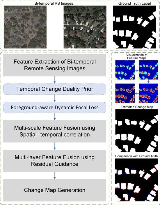
In this paper, we introduce EFP-Net, a novel approach for building change detection that utilizes effective feature fusion and foreground perception to address the aforementioned issues. Firstly, a spatial–temporal correlation module is designed to efficiently integrate features from bi-temporal images and enhance the representation capacity of change features. This module leverages the temporal change duality prior and multi-scale perception to augment the three-dimensional convolution capability to model spatial–temporal features in bi-temporal data. Secondly, to enhance hierarchical feature fusion, a residual-guided module is introduced. It optimizes shallow features guided by deep-layer change predictions, reducing noise introduced during the feature fusion process. Lastly, to address class imbalance, we further introduce a foreground-aware loss function that enables the model to focus on the challenging, sparsely distributed foreground samples.
The main contributions of the proposed EFP-Net are summarized as follows:
  • We introduce a spatial–temporal correlation module (STCM) to generate discriminative change features that can provide accurate localization of changed objects.
  • We introduce a residual-guided module (RGM) to enhance hierarchical feature fusion.
  • We propose a dynamic Focal loss with foreground awareness to address the class imbalance problem in building change detection.
Based on the STCM and RGM, we have developed EFP-Net, a novel building change detection algorithm for optical remote sensing images. Experimental results demonstrate the state-of-the-art performance of the proposed method on benchmark datasets.
The rest of the paper is organized as follows: Section 2 provides a detailed presentation of the proposed method. Section 3 presents experimental results, along with analysis and comparisons with state-of-the-art methods. Finally, Section 4 concludes the paper.

2. Methodology

Figure 1 illustrates the overall framework of the proposed EFP-Net, which consists of three main modules: the feature extraction module (FEM), the spatial–temporal correlation module (STCM), and the residual guidance module (RGM). For a pair of bi-temporal remote sensing images I T 0 , I T 1 , the network initially transforms the bi-temporal image pair into five feature pairs as the front-end of the network, denoted by { F T 0 ( i ) , F T 1 ( i ) } , where ( i ) { 1 , 2 , 3 , 4 , 5 } indicates the layer number. In our work, a Siamese VGG16 pre-trained on ImageNet [49] without its last max-pooling layer and linear layer is employed for feature extraction, referred to as FEM in the framework. The multi-scale bi-temporal features are then individually sent to the STCMs to generate highly representative multi-scale change features { F ( 1 ) , F ( 2 ) , F ( 3 ) , F ( 4 ) , F ( 5 ) } . After that, feature F ( 5 ) is directed to a lightweight head to obtain an initial change map C ( 5 ) as the guidance for subsequent shallow change features. To progressively restore the details of changing objects, the RGM is employed to suppress background noise and extract structural information within shallow features. Finally, the refined features are decoded into a final change map C ( 1 ) with a lightweight head consisting of two CBR (Convolution–Batch Normalization–Relu) units. The construction of each model is introduced in detail in the following subsections.

2.1. Feature Extraction Module

In the task of building change detection, the model takes a bi-temporal image pair as input. Currently, commonly used feature extraction network architectures can be categorized into single-input feature extraction networks and Siamese network structures. The weight-sharing strategy of Siamese network maps inputs to a unified feature space, which not only preserves the independence of bi-temporal features but also facilitates the learning of change features. Therefore, we utilize a Siamese structure for the feature extraction module. Specifically, a VGG16 pre-trained on ImageNet is adopted, with its last maximum pooling layer and the linear layer removed, as listed in Table 1. Given a pair of bi-temporal high-resolution RS images with size of 256 × 256 , the FEM can be divided into five stages (FEM1–FEM5), where each stage extracts features of a single scale. Ultimately, five pairs of bi-temporal features with different scales are obtained: { F T 0 ( i ) , F T 1 ( i ) } , where ( i ) 1 , 2 , 3 , 4 , 5 indicates the layer number.

2.2. Spatial–Temporal Correlation Module

The objective of building change detection is to acquire a binary change map from bi-temporal remote sensing images, engaging in a pixel-wise binary classification task. Recognizing that both the emergence and vanishing of change are categorized as the changed class in the change map, we introduce the temporal change duality prior as a constraint in the change detection task. This involves ensuring that the change map derived from temporal T0 to T1 aligns with the change map derived from temporal T1 to T0, as shown in Figure 2.
Based on the temporal change duality prior with multi-scale feature fusion through a multi-branch structure, we introduce a novel spatial–temporal correlation module (STCM) to address the problems of feature concatenation and algebraic operations in establishing temporal relationships and the learning of change features. The structure of the proposed STCM is illustrated in Figure 3, where F T 0 , F T 1 R C × H × W are a pair of features extracted by the FEM, where C represents the channel number, and H and W are the height and width, respectively.
In order to model the dual change features, a 4D feature map F R C × 3 × H × W is first generated through dimension expansion and alternative concatenation in the temporal dimension of feature pair F T 0 , F T 1 in each layer, expressed as follows:
F c ( i ) = Cat F T 0 ( i ) , F T 1 ( i ) , F T 0 ( i ) ; T , i { 1 , 2 , 3 , 4 , 5 } ,
where Cat ( ; T ) indicates concatenation in the temporal dimension, which is capable of preserving the high-dimensional features of each time phase.
After that, the change features with temporal change duality, denoted by F tcd , are extracted through a 3D convolution operation as follows:
F tcd ( i ) = Conv [ 2 , k , k ] ( F c ( i ) ) ,
where F tcd R 2 C × 2 × H × W and Conv [ 2 , k , k ] ( ) indicates a depth-separable 3D convolution operation with kernel size of 2 × k × k and stride of 1 in all directions. As the kernel moves along the temporal dimension, dual change information is extracted, such as F t 0 t 1 and F t 1 t 0 R 2 C × 1 × H × W .
In order to enhance the perception of multi-scale changes, we construct three parallel branches for temporal–spatial modeling, drawing inspiration from the Inception architecture [50]. Specifically, the kernel sizes of the convolution in each branch are set to 2 × 1 × 1 , 2 × 3 × 3 , and 2 × 5 × 5 , respectively. By such design, the STCM gains the capability of modeling the spatial–temporal changes of bi-temporal features.
Finally, the outputs of the three branches are combined in the channel dimension and merged through a 2 × 1 × 1 convolution operation to produce change feature F ( i ) R 2 × C × H × W as follows:
F ( i ) = Conv [ 2 , 1 , 1 ] Cat F tcd 1 , F tcd 3 , F tcd 5 ; Ch ,
where Ch represents the channel dimension.

2.3. Residual Guidance Module

As discussed in [41], shallow-level features are known to contain both structural and textural information, along with background noise. Hence, to simultaneously address the suppression of background noise and the extraction of change object details, we propose the residual guidance module (RGM). The fundamental principle behind the RGM is to eliminate irrelevant background noise and extract the details from change objects in a guided manner. Particularly, the RGM is employed in layer 1 to layer 4 by utilizing the higher-layer, predicted change map as the guidance map, which guides shallow-layer features to concentrate on potential change regions. This facilitates more efficient fusion of features across different scales.
Figure 4 demonstrates the framework of the RGM, which consists of two stages: guidance map construction and group re-fusion. Firstly, we generate a temporary map S ( 5 ) by applying a transposed convolution operation to up-sample predicted change map C ( 5 ) by 2 times. Guidance map G, representing the extent of change in the current layer, can be thus generated by normalizing S of the deeper layer, which is formulated as follows:
G ( i ) = S 1 ( i + 1 ) S 0 ( i + 1 ) + 1 2 , i { 1 , 2 , 3 , 4 }
where the superscript ( · ) denotes the layer number. S 0 ( i + 1 ) and S 1 ( i + 1 ) represent the probability of the unchanged and changed classes, respectively, which are extracted along the channel dimension from the temporary image of deeper layer S ( i + 1 ) .
After that, a group re-fusion strategy is applied to obtain a refined change feature of the current layer ( F ^ ( i ) ) by combining guidance map G ( i ) with the change feature of the current layer ( F ( i ) ). Specifically, F ( i ) is evenly split into m groups and then concatenated with guidance map G to model F ^ ( i ) as follows:
F sp ( 1 ) ( i ) , , F sp ( k ) ( i ) , , F sp ( m ) ( i ) = Split F c , k { 1 , 2 , , m } F ^ ( i ) = Cat F sp ( 1 ) ( i ) , G , , F sp ( k ) ( i ) , G , , F sp ( m ) ( i ) , G ,
where Split and Cat denote the split and concatenate operations, respectively. The subscripts sp and ( k ) indicate the split features and the index of the group, respectively. The superscript i { 1 , 2 , 3 , 4 } represents the number of the layer. With the group re-fusion strategy, dilution of guidance information during the fusion process can be effectively mitigated.
Refined change feature F ^ ( i ) is then input to a 3 × 3 convolutional layer and then added to input current-layer feature F ( i ) to generate optimized feature F ^ opt ( i ) , which can be expressed as follows:
F ^ opt ( i ) = F ( i ) + Conv [ 3 , 3 ] ( F ^ ( i ) ) ,
where Conv [ 3 , 3 ] ( · ) represents a 2D convolution operation with the size of 3 × 3 and the stride of 1.
By employing this strategy, shallow features guided by the deep prediction map are capable of effectively suppressing irrelevant background noise. This approach facilitates more efficient integration of features across multiple levels, thereby enhancing the restoration of detailed information specific to the changing object.

2.4. Loss Function

In change detection, Focal loss [51] is widely employed to address the class imbalance problem between the changed foreground and the background, which can be expressed as follows:
L focal ( p , y ) = 1 N i , y i = 1 n p α 1 p i γ log p i + j , y j = 0 n n ( 1 α ) p j γ log 1 p j ,
where p and y denote the predicted change probability map and the corresponding label values, respectively. N = H × W represents the total pixel number of the samples with label y; n p denotes the number of positive samples (changed foreground); and n n indicates the number of negative samples (unchanged background).
Given that α = α if y = 1 ; 1 α otherwise and p i = p i if y = 1 ; 1 p i otherwise , Equation (7) can be subsequently simplified as follows:
L focal ( p , y ) = 1 N i = 1 N α i 1 p i γ log p i
where α ( 0 , 1 ) is a constant weight factor designed to augment the loss weight of positive samples. The term 1 p i γ serves as a dynamic weight factor, with γ functioning as the modulation factor. The value of p reflects the degree of difficulty in classifying the current sample. It is noteworthy to mention that dynamic weight term 1 p i γ is determined by the model’s output. As a consequence, the estimation of foreground samples would be imprecise, since the model’s discriminative capability might remain ambiguous during the initial training stage. Additionally, larger weights assigned to foreground samples might also compromise the model’s convergence efficiency.
To account for this, we suggest dynamically adjusting the weights of individual samples in the cross-entropy loss according to the training iteration. Specifically, we incorporate an annealing function into the modulation factor for a more agile learning paradigm. This approach enables the weights to be fine-tuned based on the changing conditions throughout the training period, thereby enhancing the model’s ability to perceive changes in the foreground. The proposed dynamic Focal loss is formulated as follows:
L df ( p , y ) = 1 N i = 1 N M i + ψ ( t ) 1 M i log p i ,
where M i = α i 1 p i γ . ψ t [ 0 , 1 ] represents the Cosine annealing function with the number of training iterations (t) as a variable, which is defined as follows:
ψ t = 0.5 1 + cos t T max π ,
where t and T max denote the current training step and the maximum annealing step, respectively. By leveraging dynamic weighting that adaptively adjusts with training cycles, the model gradually focuses on the hard samples, which effectively addresses the inherent issue of class imbalance.
Throughout the training process, predictions of changes are output at five different levels. Therefore, the overall loss function is formulated by calculating the total loss between the five change prediction maps and the ground-truth change map, which is expressed as follows:
L = i = 1 5 β ( i ) L df ( i ) ,
where L d f ( i ) and β ( i ) denote the loss of the prediction and the corresponding weight in the i-th layer, respectively.

3. Experiments

3.1. Experimental Datasets

The proposed EFP-Net is evaluated on three public change detection datasets: LEVIR-CD [34], WHU-BCD [4], LEVIR-CD [34], and CDD [52].
The LEVIR-CD is open-sourced by the LEVIR Lab of Beihang University and was collected in Texas, USA, between 2002 and 2018. It consists of 637 high-resolution bi-temporal image pairs, each with a spatial resolution of 0.5 m and a resolution of 1024 × 1024. LEVIR-CD contains various types of buildings, ranging from single-story houses and large warehouses to upscale apartments. The buildings undergoing change in the images are small and densely packed. Given the considerable time span between the image acquisition dates, achieving precise detection of building changes presents a significant challenge. In the original work [34], each image was non-overlappingly cropped into 16 sub-images of 256 × 256. By default, the dataset was partitioned into training, validation, and test sets, comprising 445, 64, and 128 images, respectively. For fair comparisons with other methods, the training, validation, and test sets are created by cropping non-overlapping patches into 7120, 1024, and 2048 samples, respectively.
The WHU-BCD dataset is composed of a pair of bi-temporal remote sensing images with size of 15,354 × 32,507 and a spatial resolution of 0.2 m. These images were collected in the southwestern region of Queensland in 2012 and 2016, respectively. The original images are cropped into 256 × 256 sub-images with a stride of 256. The sub-images are then randomly divided according to the ratio of 7:1:2, resulting in train/val/test sets comprising 5534, 762, and 1524 image pairs, respectively.
The CDD dataset comprises 11 image pairs, with specific resolutions ranging from 3 cm to 100 cm. Four of these pairs have a resolution of 1900 × 1000, while the remaining pairs are 4725 × 2200. CDD contains the change information of various land cover types, including vehicles, buildings, roads, etc. It is characterized by considerable variations in season, climate, and weather conditions. Following the original work, the raw images were segmented into non-overlapping sub-images of 256 × 256, yielding a total of 16,000 image pairs. Out of these, 10,000 pairs were designated for the training set, 3000 pairs for the validation set, and the remaining 3000 pairs for the test set.
Figure 5 and Table 2 illustrate some samples of the bi-temporal images with ground-truth labels and summary information of the selected remote sensing image datasets for building change detection, respectively.

3.2. Implementation Details

We trained and tested our network on Ubuntu 18.04 with an Intel E5-2640 CPU and an Nvidia GTX 1080Ti GPU using PyTorch 1.12.0. We employed the Adam optimizer and set β 1 , β 2 of the momentum to 0.5 and 0.9, respectively. The batch size was configured to 12, and the learning rate was initially set to 1 × 10 4 . The model was trained for 120 epochs for all datasets. To mitigate the risk of over-fitting and enhance the generalization capabilities, data augmentation techniques such as random mirroring, flipping, and rotation were employed during the training stage.
In order to fully evaluate the performance of the proposed EFP-Net both qualitatively and quantitatively, seven SOTA approaches for building change detection were selected for comparison, including FC-EF [31], FC-Siam-conc [31], FC-Siam-diff [31], IFNet [53], SNUNet-CD [33], BIT [39], and ChangeFormer [40].
We summarized the main characteristics of all compared methods in terms of network structure, change feature learning method, hierarchical feature fusion method, and the loss functions, as listed in Table 3. In the table, Single and Siamese refer to the single-stream feature extraction network and Siamese feature extraction network, respectively. Cat represents the concatenate operation, and 1 stands for the 1 distance. SA denotes spatial attention, and CA refers to channel attention. CE, WCE, and DICE are the cross-entropy loss, the weighted cross-entropy loss, and the Dice loss, respectively.

3.3. Evaluation Metrics

In the experiments, five frequently utilized evaluation metrics were adopted: overall accuracy (OA), Precision, Recall, F1-score (F1), and intersection over union (IoU). The calculations for each indicator are defined as follows:
O A = T P + T N T P + T N + F P + F N ,
P r e c i s i o n = T P T P + F P ,
R e c a l l = T P T P + F N ,
F 1 = 2 × P r e c i s i o n × R e c a l l P r e c i s i o n + R e c a l l ,
I o U = T P T P + F N + F P ,
where TP (true positive) indicates pixels of the changed objects correctly predicted as the ‘change’ category. TN (true negative) represents pixels of the unchanged objects correctly predicted as the ‘unchange’ category. FP (false positive) means that pixels remaining unchanged are mistakenly predicted as the ‘change’ category. FN (false negative) indicates that changed pixels are incorrectly predicted as the ‘unchange’ category.

3.4. Experimental Results

Figure 6, Figure 7 and Figure 8 illustrate the comparison results of different methods on LEVIR-CD, WHU-BCD, and CDD, respectively. It is intuitively observed in Figure 6 that the results of SNUNet-CD, FC-Siam-diff, FC-Siam-conc, and KC-EF contain obvious false detections (indicated in blue and red). On the other hand, ChangeFormer, BIT, IFNet, and the proposed EFP-Net achieve satisfying results, and our method has better performance in extracting the interior structure of changed buildings. Overall, the results of the proposed method align with the ground truth most closely and outperform others in detecting changed building targets of varying scales and resisting interference from false changes. This is due to the employment of the STCM, which captures the contextual relationship between single-pixel values and multi-scale regions, enhancing the representation of change features and ensuring the integrity of changed objects. In addition, the RGM optimizes shallow features with the guidance of deep prediction maps, effectively reducing false detections caused by background noise, thereby achieving accurate detection around the edges of changing objects.
In Figure 7, it is observed that compared with other methods, EFP-Net significantly reduces instances of missed and false detections while preserving the integrity of large-scale buildings. Specifically, as observed in the first row of Figure 7, obvious false detections (FN, indicated in blue) can be noted in the results of all the compared methods. Furthermore, false negative detections (indicated in red) are generated by FC-Siam-diff, FC-Siam-conc, and KC-EF. While both EFP-Net and ChangeFormer have better performance, our EFP-Net generates fewer false detections. It is also noted that EFP-Net not only accurately achieves multi-scale change detection results in scenes with highly similar structures but also maintains the integrity of building interiors. As evidenced in both the first and last rows of Figure 7, EFP-Net demonstrates remarkable resistance to false changes, with its detection results aligning with the reference labels most closely when compared with other methods.
Compared with the LEVIR-CD and WHU-BCD datasets, CDD not only contains changes in buildings but also includes changes in vehicles, roads, trees, etc. As shown in Figure 8, EFP-Net is capable of achieving detailed change detection with high-quality change maps for both smaller areas like trees and vehicles, and complex areas like roads and buildings.
Based on above qualitative comparisons, it is evident that the STCM is capable of establishing contextual connections between individual pixel points and multi-scale regions, which significantly enhances the representational capacity for features depicting change, ensuring the preservation of the integrity of buildings. Concurrently, the RGM demonstrates its effectiveness in background noise suppression through guided optimization of shallow features, resulting in a notable reduction in false detections. This contributes to the precision in detecting edge pixels of changing structures and preserves the internal integrity of buildings.
In addition to subjective comparisons, we also conducted quantitative evaluations on the datasets LEVIR-CD, WHU-BCD, and CDD, as demonstrated in Table 4, Table 5 and Table 6, respectively. ↑ indicates that performance improves as the score increases, and the best score is marked in bold. As illustrated in Table 4, the proposed EFP-Net consistently outperforms the other compared methods in all evaluated metrics on the LEVIR-CD dataset, with respective values of 99.10%, 92.18%, 90.15%, 83.74%, and 91.15%. In particular, compared with the second-best model, ChangeFormer, our EFP-Net improves the values of overall accuracy, Precision, Recall, IoU, and F1-score by 0.06%/0.13%/1.35%/1.26%/0.75%, respectively. While ChangeFormer utilizes a Transformer architecture to establish global contextual relationships, its ability to represent change features is constrained by its straightforward feature concatenation strategy, resulting in a lower Recall score. The enhanced performance of our method in the Recall metric is mainly attributed to the specially designed STCM, which effectively leverages the spatial–temporal information of bi-temporal features. Moreover, the proposed RGM effectively mitigates background noise, leading to an improved Precision score. Table 5 shows the performance evaluations on the WHU-BCD dataset. It is noted that the proposed EFP-Net exhibits remarkable results on scenes with highly similar structures. The EFP-Net consistently outperforms the compared models in all the metrics. Specifically, with regard to the Recall metric, EFP-Net surpasses the second-ranked model by 3.98%, which suggests the better capability of our method in accurately detecting building changes and subsequently reducing missed detections. Additionally, in the context of mitigating false detections, EFP-Net reaches a notable Precision score of 93.42%. Table 6 further gives the performance evaluations on the CDD dataset. It can be observed that EFP-Net outperforms other methods across all metrics in diverse scenarios. Consequently, both qualitative and quantitative comparisons demonstrate the effectiveness and generalizability of the proposed EFP-Net.

3.5. Ablation Study

In order to verify the effectiveness of the proposed modules and the dynamic Focal loss, we performed ablation experiments by incrementally introducing the STCM, RGM, and dynamic Focal (DF) loss into the baseline model. The ablation experiments were carried out on all the three datasets, as demonstrated in Table 7, Table 8 and Table 9, respectively. Specifically, the ’baseline’ model was constructed by replacing the STCM with a standard feature concatenate operation and removing the RGM. We also employed cross-entropy as the loss function in the baseline model.

3.5.1. Verification of Modules

As observed in the second row of each table, with the integration of the STCM, the model demonstrated notable advances in learning the dynamic changes between bi-temporal features, which is evidenced by the improvements in the metric values. Specifically, as illustrated in Table 7 relative the verification on LEVIR-CD, compared with the baseline model, the values of OA, Precision, Recall, IoU, and F1 increased by 0.25%, 2.58%, 1.44%, 3.84%, and 2.00%, respectively. Improvements can also be observed in the ablation results on WHU-BCD and CDD, as listed in Table 8 and Table 9, respectively. On the WHU-BCD dataset, the incorporation of the STCM increases the value of OA, Precision, Recall, IoU, and F1 by 1.45%, 2.66%, 0.32%, 1.86%, and 1.46%, respectively. Meanwhile, on the CDD dataset, the increases are 0.62%, 1.17%, 1.22%, 3.44%, and 1.19%, respectively. This is primarily because the STCM utilizes the temporal change duality prior and multi-scale perception to augment the three-dimensional convolution capability, which is more robust in obtaining discriminative change features.
As mentioned previously, the RGM leverages deep-layer change map predictions to fine-tune shallow-layer change features, which strategically directs the model’s focus towards areas of significant change while suppressing background noise. As observed in the second row of each table, compared with the baseline, the integration of the RGM increased the values of OA, Precision, Recall, IoU, and F1 by 0.39%, 2.72%, 1.97%, 3.98%, and 2.33% on LEVIR-CD; by 1.27%, 3.46%, 3.10%, 2.30%, and 3.28% on WHU-BCD; and by 0.73%, 0.93%, 1.08%, 3.57%, and 1.00% on CDD. The performance improvement is a result of the RGM’s effective fusion of multi-layer features, whereby it suppresses background noise guided by the deep prediction map, ensuring that the detailed information of the change object is accurately restored.
With both STCM and RGM added, the ’baseline + STCM + RGM’ configuration yields further improvements in OA, Precision, Recall, IoU, and F1 by 0.52%, 3.14%, 2.48%, 4.33%, and 2.8% on LEVIR-CD; 2.06%, 4.08%, 3.16%, 3.53%, and 3.61% on WHU-BCD; 1.64%, 3.36%, 1.52%, 3.7%, and 2.44% on CDD. Furthermore, the model shows significant improvements under the constraint of the proposed dynamic Focal loss. Compared with the baseline model, the proposed EFP-Net demonstrates significant enhancements in the metrics of OA, Precision, Recall, IoU, and F1, with improvements of 0.57%, 3.45%, 3.05%, 5.07%, and 3.24%, respectively.
We also present visualizations of the refined feature maps generated by the RGM on LEVIR-CD. Figure 9a,b display a pair of bi-temporal RS images, while (c) and (d) are the ground-truth label and the predicted change maps of EFP-Net, respectively. Figure 9e–h are the feature maps derived from ‘baseline’, ‘baseline’ + STCM, ‘baseline’ + RGM, and EFP-Net, respectively.
The comparison between Figure 9e,f demonstrates improved confidence in detecting building changes, which proves the effectiveness of the STCM in reducing background noise and identifying building change locations. Similarly, it is observed in the comparison between Figure 9e,g that integrating the RGM enhances the network’s capability to recover the fine details of changed buildings. Furthermore, Figure 9h reveals that the incorporation of both the STCM and RGM further enhances the contrast between changed buildings and the background. These observations collectively offer compelling evidence of the effectiveness of the proposed STCM and RGM.

3.5.2. Verification of Loss Function

We also verified the effectiveness of the proposed dynamic Focal (DF) loss. As observed in the last two rows of Table 7, Table 8 and Table 9, the performance of the ‘baseline’ + STCM + RGM model is further improved under the constraint of the DF loss. This is because the proposed DF loss enables the model to focus on the changing foreground samples during training, thereby mitigating the impact of class imbalance on model performance.
In addition, we also compared the effectiveness of the proposed dynamic Focal loss with other loss functions commonly used in change detection on LEVIR-CD. In particular, cross-entropy (CE) loss, weighted cross-entropy (WCE) loss, and Focal loss were employed for comparisons. As shown in Table 10, compared with the CE loss, the WCE loss enhances the weights of the loss for a small number of foreground samples, resulting in an improvement in the Recall metric. The Recall metric is further improved with the Focal loss, as it reduces the weights assigned to easily classified samples. Relative to other loss functions, the proposed DF loss achieves the best scores across all the metrics, demonstrating its effectiveness.

3.5.3. Verification of Parameter

In the RGM, higher-layer features F c h are evenly split in to g groups and then concatenated with G to model the initial change feature, F c . We also verified the impact of the number of groups g in the RGM on the performance of the EFP-Net. Specifically, experiments were carried out with g values of 1, 2, 4, 8, 16, and 32. As revealed in Table 11, the performance of the model improves progressively as the value of g increases and peaks when the value of g reaches eight. However, the performance of the model starts to decline as the value of g continues to increase, implying that an excessive number of groups leads to redundancy in F c . Consequently, we fixed the number of groups at eight in our experiments.

4. Conclusions

In this article, we introduce EFP-Net, a novel building change detection network based on efficient feature fusion and foreground perception. We developed the spatial–temporal correlation module (STCM) and the residual guidance module (RGM) to enhance the fusion of bi-temporal and hierarchical features, respectively. The STCM utilizes temporal change duality and multi-scale perception to refine the modeling of temporal changes in bi-temporal features from both temporal and spatial dimensions. The RGM, on the other hand, employs deep-layer change map predictions to optimize shallow-layer features, concentrating on potential change areas and reducing noise introduction during the hierarchical feature fusion process. Additionally, we introduce foreground-aware dynamic Focal loss to address the class imbalance problem inherent in building change detection. Comparative experiments with other state-of-the-art deep learning-based methods demonstrate that the proposed EFP-Net has remarkable performance in preserving the details of building change and reducing false detections. In our study, we also found that existing methods attain satisfactory performance when trained on abundant data; however, their efficacy significantly declines when applied to new scenes. Given that creating datasets for each unique scene is impractical, our future work will focus on investigating domain-adaptive building change detection methods, which aim to utilize solely existing annotated data to facilitate seamless adaptability to new scenes, consequently reducing the training costs.

Author Contributions

Conceptualization, W.L. and R.H.; methodology, W.L.; validation, R.H. and Y.D.; writing—original draft preparation, R.H. and W.L.; writing—review and editing, R.H. and S.M.; visualization, W.L.; supervision, M.H.; funding acquisition, R.H. All authors have read and agreed to the published version of the manuscript.

Funding

This research was funded by the National Natural Science Foundation of China: 62001396; the RSP National Key Laboratory (Grant No. JKW202206); and the Key Research and Development Program of Shaanxi (Grant No. 2022ZDLGY06-08, 2023-ZDLGY-46).

Data Availability Statement

Public datasets were employed in this study. The LEVIR-CD dataset can be found at https://justchenhao.github.io/LEVIR/, accessed on 10 June 2021. The WHU-BCD dataset can be found at https://study.rsgis.whu.edu.cn/pages/download/building_dataset.html, accessed on 10 June 2021. The CDD dataset can be found at https://drive.google.com/file/d/1GX656JqqOyBi_Ef0w65kDGVto-nHrNs9/edit, accessed on 2 July 2021.

Conflicts of Interest

The authors declare no conflict of interest.

References

  1. Zhang, Y.; Fu, L.; Li, Y.; Zhang, Y. Hdfnet: Hierarchical dynamic fusion network for change detection in optical aerial images. Remote Sens. 2021, 13, 1440. [Google Scholar] [CrossRef]
  2. Liu, M.; Chai, Z.; Deng, H.; Liu, R. A CNN-transformer network with multiscale context aggregation for fine-grained cropland change detection. IEEE J. Sel. Top. Appl. Earth Obs. Remote Sens. 2022, 15, 4297–4306. [Google Scholar] [CrossRef]
  3. Yang, X.; Lv, Z.; Atli Benediktsson, J.; Chen, F. Novel Spatial–Spectral Channel Attention Neural Network for Land Cover Change Detection with Remote Sensed Images. Remote Sens. 2022, 15, 87. [Google Scholar] [CrossRef]
  4. Ji, S.; Wei, S.; Lu, M. Fully convolutional networks for multisource building extraction from an open aerial and satellite imagery data set. IEEE Trans. Geosci. Remote Sens. 2018, 57, 574–586. [Google Scholar] [CrossRef]
  5. Huang, X.; Han, X.; Ma, S.; Lin, T.; Gong, J. Monitoring ecosystem service change in the City of Shenzhen by the use of high-resolution remotely sensed imagery and deep learning. Land Degrad. Dev. 2019, 30, 1490–1501. [Google Scholar] [CrossRef]
  6. Pang, L.; Sun, J.; Chi, Y.; Yang, Y.; Zhang, F.; Zhang, L. CD-TransUNet: A Hybrid Transformer Network for the Change Detection of Urban Buildings Using L-Band SAR Images. Sustainability 2022, 14, 9847. [Google Scholar] [CrossRef]
  7. Liu, S.; Chi, M.; Zou, Y.; Samat, A.; Benediktsson, J.A.; Plaza, A. Oil spill detection via multitemporal optical remote sensing images: A change detection perspective. IEEE Geosci. Remote Sens. Lett. 2017, 14, 324–328. [Google Scholar] [CrossRef]
  8. Zheng, Z.; Zhong, Y.; Wang, J.; Ma, A.; Zhang, L. Building damage assessment for rapid disaster response with a deep object-based semantic change detection framework: From natural disasters to man-made disasters. Remote Sens. Environ. 2021, 265, 112636. [Google Scholar] [CrossRef]
  9. Wang, T.; Shi, Q.; Nikkhoo, M.; Wei, S.; Barbot, S.; Dreger, D.; Bürgmann, R.; Motagh, M.; Chen, Q.F. The rise, collapse, and compaction of Mt. Mantap from the 3 September 2017 North Korean nuclear test. Science 2018, 361, 166–170. [Google Scholar] [CrossRef]
  10. Pu, R.; Landry, S. Evaluating seasonal effect on forest leaf area index mapping using multi-seasonal high resolution satellite pléiades imagery. Int. J. Appl. Earth Obs. Geoinf. 2019, 80, 268–279. [Google Scholar] [CrossRef]
  11. Gao, Y.; Gao, F.; Dong, J.; Wang, S. Transferred deep learning for sea ice change detection from synthetic-aperture radar images. IEEE Geosci. Remote Sens. Lett. 2019, 16, 1655–1659. [Google Scholar] [CrossRef]
  12. Wang, J.; Yang, D.; Detto, M.; Nelson, B.W.; Chen, M.; Guan, K.; Wu, S.; Yan, Z.; Wu, J. Multi-scale integration of satellite remote sensing improves characterization of dry-season green-up in an Amazon tropical evergreen forest. Remote Sens. Environ. 2020, 246, 111865. [Google Scholar] [CrossRef]
  13. Mondini, A.; Guzzetti, F.; Reichenbach, P.; Rossi, M.; Cardinali, M.; Ardizzone, F. Semi-automatic recognition and mapping of rainfall induced shallow landslides using optical satellite images. Remote Sens. Environ. 2011, 115, 1743–1757. [Google Scholar] [CrossRef]
  14. Marchesi, S.; Bruzzone, L. ICA and kernel ICA for change detection in multispectral remote sensing images. In Proceedings of the 2009 IEEE International Geoscience and Remote Sensing Symposium, Cape Town, South Africa, 12–17 July 2009; Volume 2, pp. 980–983. [Google Scholar]
  15. Kuncheva, L.I.; Faithfull, W.J. PCA feature extraction for change detection in multidimensional unlabeled data. IEEE Trans. Neural Netw. Learn. Syst. 2013, 25, 69–80. [Google Scholar] [CrossRef] [PubMed]
  16. Celik, T. Unsupervised change detection in satellite images using principal component analysis and k-means clustering. IEEE Geosci. Remote Sens. Lett. 2009, 6, 772–776. [Google Scholar] [CrossRef]
  17. Wu, C.; Du, B.; Zhang, L. Slow feature analysis for change detection in multispectral imagery. IEEE Trans. Geosci. Remote Sens. 2013, 52, 2858–2874. [Google Scholar] [CrossRef]
  18. Yang, Z.; Qin, Q.; Zhang, Q. Change detection in high spatial resolution images based on support vector machine. In Proceedings of the 2006 IEEE International Symposium on Geoscience and Remote Sensing, Denver, CO, USA, 31 July–4 August 2006; pp. 225–228. [Google Scholar]
  19. Tan, K.; Du, P. Hyperspectral remote sensing image classification based on support vector machine. J. Infrared Millim. Waves 2008, 27, 123–128. [Google Scholar] [CrossRef]
  20. Liu, D.; Song, K.; Townshend, J.R.; Gong, P. Using local transition probability models in Markov random fields for forest change detection. Remote Sens. Environ. 2008, 112, 2222–2231. [Google Scholar] [CrossRef]
  21. Zhang, Z.; Zhang, X.; Xin, Q.; Yang, X. Combining the pixel-based and object-based methods for building change detection using high-resolution remote sensing images. Acta Geod. Et Cartogr. Sin. 2018, 47, 102. [Google Scholar]
  22. Krizhevsky, A.; Sutskever, I.; Hinton, G.E. Imagenet classification with deep convolutional neural networks. Commun. ACM 2017, 60, 84–90. [Google Scholar] [CrossRef]
  23. Long, J.; Shelhamer, E.; Darrell, T. Fully convolutional networks for semantic segmentation. In Proceedings of the IEEE Conference on Computer Vision and Pattern Recognition, Boston, MA, USA, 7–12 June 2015; pp. 3431–3440. [Google Scholar]
  24. Mathis, A.; Mamidanna, P.; Cury, K.M.; Abe, T.; Murthy, V.N.; Mathis, M.W.; Bethge, M. DeepLabCut: Markerless pose estimation of user-defined body parts with deep learning. Nat. Neurosci. 2018, 21, 1281–1289. [Google Scholar] [CrossRef] [PubMed]
  25. Zhao, Z.Q.; Zheng, P.; Xu, S.t.; Wu, X. Object detection with deep learning: A review. IEEE Trans. Neural Networks Learn. Syst. 2019, 30, 3212–3232. [Google Scholar] [CrossRef] [PubMed]
  26. Deng, J.; Wang, K.; Deng, Y.; Qi, G. PCA-based land-use change detection and analysis using multitemporal and multisensor satellite data. Int. J. Remote Sens. 2008, 29, 4823–4838. [Google Scholar] [CrossRef]
  27. Zhuang, H.; Deng, K.; Fan, H.; Yu, M. Strategies combining spectral angle mapper and change vector analysis to unsupervised change detection in multispectral images. IEEE Geosci. Remote Sens. Lett. 2016, 13, 681–685. [Google Scholar] [CrossRef]
  28. Li, Q.; Huang, X.; Wen, D.; Liu, H. Integrating multiple textural features for remote sensing image change detection. Photogramm. Eng. Remote Sens. 2017, 83, 109–121. [Google Scholar] [CrossRef]
  29. Wu, C.; Du, B.; Cui, X.; Zhang, L. A post-classification change detection method based on iterative slow feature analysis and Bayesian soft fusion. Remote Sens. Environ. 2017, 199, 241–255. [Google Scholar] [CrossRef]
  30. Shi, W.; Zhang, M.; Zhang, R.; Chen, S.; Zhan, Z. Change detection based on artificial intelligence: State-of-the-art and challenges. Remote Sens. 2020, 12, 1688. [Google Scholar] [CrossRef]
  31. Daudt, R.C.; Le Saux, B.; Boulch, A. Fully convolutional siamese networks for change detection. In Proceedings of the IEEE International Conference on Image Processing, Athens, Greece, 7–10 October 2018; pp. 4063–4067. [Google Scholar]
  32. Peng, X.; Zhong, R.; Li, Z.; Li, Q. Optical remote sensing image change detection based on attention mechanism and image difference. IEEE Trans. Geosci. Remote Sens. 2020, 59, 7296–7307. [Google Scholar] [CrossRef]
  33. Fang, S.; Li, K.; Shao, J.; Li, Z. SNUNet-CD: A densely connected Siamese network for change detection of VHR images. IEEE Geosci. Remote Sens. Lett. 2021, 19, 8007805. [Google Scholar] [CrossRef]
  34. Chen, H.; Shi, Z. A spatial-temporal attention-based method and a new dataset for remote sensing image change detection. Remote Sens. 2020, 12, 1662. [Google Scholar] [CrossRef]
  35. Chen, J.; Yuan, Z.; Peng, J.; Chen, L.; Huang, H.; Zhu, J.; Liu, Y.; Li, H. DASNet: Dual attentive fully convolutional Siamese networks for change detection in high-resolution satellite images. IEEE J. Sel. Top. Appl. Earth Obs. Remote Sens. 2020, 14, 1194–1206. [Google Scholar] [CrossRef]
  36. Maiya, S.R.; Babu, S.C. Slum segmentation and change detection: A deep learning approach. In Proceedings of the Conference on Neural Information Processing Systems, Montreal, QC, USA, 3–8 December 2018; pp. 1–5. [Google Scholar]
  37. Zhang, C.; Wei, S.; Ji, S.; Lu, M. Detecting large-scale urban land cover changes from very high resolution remote sensing images using CNN-based classification. ISPRS Int. J. Geo-Inf. 2019, 8, 189. [Google Scholar] [CrossRef]
  38. Ji, S.; Shen, Y.; Lu, M.; Zhang, Y. Building instance change detection from large-scale aerial images using convolutional neural networks and simulated samples. Remote Sens. 2019, 11, 1343. [Google Scholar] [CrossRef]
  39. Chen, H.; Qi, Z.; Shi, Z. Remote sensing image change detection with transformers. IEEE Trans. Geosci. Remote Sens. 2021, 60, 5607514. [Google Scholar] [CrossRef]
  40. Bandara, W.G.C.; Patel, V.M. A transformer-based siamese network for change detection. In Proceedings of the IEEE International Geoscience and Remote Sensing Symposium, Kuala Lumpur, Malaysia, 17–22 July 2022; pp. 207–210. [Google Scholar]
  41. Rao, Z.; Dai, Y.; Shen, Z.; He, R. Rethinking training strategy in stereo matching. IEEE Trans. Neural Netw. Learn. Syst. 2022, 34, 7796–7809. [Google Scholar] [CrossRef]
  42. Xu, H.; He, M.; Rao, Z.; Li, W. Him-net: A new neural network approach for sar and optical image template matching. In Proceedings of the 2021 IEEE International Conference on Image Processing (ICIP), Anchorage, AK, USA, 19–22 September 2021; pp. 3827–3831. [Google Scholar]
  43. Zhan, Y.; Fu, K.; Yan, M.; Sun, X.; Wang, H.; Qiu, X. Change detection based on deep siamese convolutional network for optical aerial images. IEEE Geosci. Remote Sens. Lett. 2017, 14, 1845–1849. [Google Scholar] [CrossRef]
  44. Wang, M.; Tan, K.; Jia, X.; Wang, X.; Chen, Y. A deep siamese network with hybrid convolutional feature extraction module for change detection based on multi-sensor remote sensing images. Remote Sens. 2020, 12, 205. [Google Scholar] [CrossRef]
  45. Zhang, M.; Shi, W. A feature difference convolutional neural network-based change detection method. IEEE Trans. Geosci. Remote Sens. 2020, 58, 7232–7246. [Google Scholar] [CrossRef]
  46. Milletari, F.; Navab, N.; Ahmadi, S.A. V-net: Fully convolutional neural networks for volumetric medical image segmentation. In Proceedings of the 2016 Fourth International Conference on 3D Vision (3DV), Stanford, CA, USA, 25–28 October 2016; pp. 565–571. [Google Scholar]
  47. Hadsell, R.; Chopra, S.; LeCun, Y. Dimensionality reduction by learning an invariant mapping. In Proceedings of the 2006 IEEE Computer Society Conference on Computer Vision and Pattern Recognition (CVPR’06), New York, NY, USA, 17–22 June 2006; Volume 2, pp. 1735–1742. [Google Scholar]
  48. Schroff, F.; Kalenichenko, D.; Philbin, J. Facenet: A unified embedding for face recognition and clustering. In Proceedings of the IEEE Conference on Computer Vision and Pattern Recognition, Boston, MA, USA, 7–12 July 2015; pp. 815–823. [Google Scholar]
  49. Simonyan, K.; Zisserman, A. Very Deep Convolutional Networks for Large-Scale Image Recognition. In Proceedings of the International Conference on Learning Representations, San Diego, CA, USA, 7–9 May 2015; pp. 1–14. [Google Scholar]
  50. Szegedy, C.; Vanhoucke, V.; Ioffe, S.; Shlens, J.; Wojna, Z. Rethinking the inception architecture for computer vision. In Proceedings of the IEEE Conference on Computer Vision and Pattern Recognition, Las Vegas, NV, USA, 27–30 June 2016; pp. 2818–2826. [Google Scholar]
  51. Lin, T.Y.; Goyal, P.; Girshick, R.; He, K.; Dollár, P. Focal loss for dense object detection. In Proceedings of the IEEE International Conference on Computer Vision, Venice, Italy, 22–29 October 2017; pp. 2980–2988. [Google Scholar]
  52. Lebedev, M.; Vizilter, Y.; Vygolov, O.; Knyaz, V.; Rubis, A. Change Detection in Remote Sensing Images Using Conditional Adversarial Networks. ISPRS-Int. Arch. Photogramm. Remote Sens. Spat. Inf. Sci. 2018, 422, 565–571. [Google Scholar] [CrossRef]
  53. Zhang, C.; Yue, P.; Tapete, D.; Jiang, L.; Shangguan, B.; Huang, L.; Liu, G. A deeply supervised image fusion network for change detection in high resolution bi-temporal remote sensing images. ISPRS J. Photogramm. Remote Sens. 2020, 166, 183–200. [Google Scholar] [CrossRef]
Figure 1. Framework of the proposed EFP-Net.
Remotesensing 15 05268 g001
Figure 2. Temporal change duality prior in building change detection.
Remotesensing 15 05268 g002
Figure 3. The architecture of the proposed STCM.
Remotesensing 15 05268 g003
Figure 4. The structure of the proposed RGM.
Remotesensing 15 05268 g004
Figure 5. Samples of the experimental datasets.
Remotesensing 15 05268 g005
Figure 6. Comparisons on the LEVIR-CD dataset. (a) T0 image; (b) T1 image; (c) ground truth; (d) proposed EFP-Net; (e) ChangeFormer [40]; (f) SNUNet-CD [33]; (g) BIT [39]; (h) IFNet [53]; (i) FC-Siam-diff [31]; (j) FC-Siam-conc [31]; (k) FC-EF [31]. Colors assigned: TP in white, TN in black, FP in red, and FN in blue.
Remotesensing 15 05268 g006
Figure 7. Comparisons on the WHU-BCD dataset. (a) T0 image; (b) T1 image; (c) ground truth; (d) proposed EFP-Net; (e) ChangeFormer [40]; (f) SNUNet-CD [33]; (g) BIT [39]; (h) IFNet [53]; (i) FC-Siam-diff [31]; (j) FC-Siam-conc [31]; (k) FC-EF [31]. Colors assigned: TP in white, TN in black, FP in red, and FN in blue.
Remotesensing 15 05268 g007
Figure 8. Comparisons on the CDD dataset. (a) T0 image; (b) T1 image; (c) ground truth; (d) proposed EFP-Net; (e) ChangeFormer [40]; (f) SNUNet-CD [33]; (g) BIT [39]; (h) IFNet [53]; (i) FC-Siam-diff [31]; (j) FC-Siam-conc [31]; (k) FC-EF [31]. Colors assigned: TP in white, TN in black, FP in red, and FN in blue.
Remotesensing 15 05268 g008
Figure 9. Comparisons of visualized feature maps.
Remotesensing 15 05268 g009
Table 1. Structure of the FEM.
NameLayerParameterOutput ResolutionOutput Channel
FE1Conv(3 × 3, 64) × 2256 × 25664
maxpool2 × 2, stride 2128 × 12864
FE2Conv(3 × 3, 128) × 2128 × 128128
maxpool2 × 2, stride 264 × 64128
FE3Conv(3 × 3, 256) × 264 × 64256
maxpool2 × 2, stride 232 × 32256
FE4Conv(3 × 3, 512) × 332 × 32512
maxpool2 × 2, stride 216 × 16512
FE5Conv(3 × 3, 512) × 316 × 16512
Table 2. Summary of selected datasets.
DatasetOriginal SizeResolution (m)Patch SizeTotal PairsTrainingValidationTest
LEVIR-CD1024 × 10240.5256 × 25610,192712010242048
WHU-BCD15,354 × 32,5070.2256 × 256782055347621524
CDD256 × 2560.03–1256 × 25616,00010,00030003000
Table 3. Characteristics of compared methods.
MethodStructureChange Feature LearningHierarchical Feature FusionLoss
FC-EF [31]Single-CatWCE
FC-Siam-conc [31]SiameseCatCatWCE
FC-Siam-diff [31]Siamese 1 CatWCE
IFN [31]SiameseCatSA, CA, CatWCE, DICE
BIT [39]Siamese 1 -CE
SNUNet-CD [33]SiameseCatCatWCE, DICE
ChangeFormer [40]SiameseCatCatCE
Table 4. Performance comparison on LEVIR-CD.
MethodOA↑Precision↑Recall↑IoU↑F1↑
FC-EF [31]97.66%83.82%67.05%59.37%74.50%
FC-Siam-conc [31]98.31%88.30%77.13%69.98%82.34%
FC-Siam-diff [31]97.40%90.74%54.47%51.60%68.07%
IFN [31]98.89%89.80%88.21%80.18%89.00%
BIT [39]98.98%90.33%89.56%81.72%89.94%
SNUNet-CD [33]98.90%89.93%88.41%80.44%89.16%
ChangeFormer [40]99.04%92.05%88.80%82.48%90.40%
EFP-Net (ours)99.10%92.18%90.15%83.74%91.15%
Table 5. Performance comparison on WHU-BCD.
MethodOA↑Precision↑Recall↑IoU↑F1↑
FC-EF [31]97.80%78.06%74.06%61.30%76.01%
FC-Siam-conc [31]95.90%54.19%83.16%48.83%65.62%
FC-Siam-diff [31]94.23%43.31%73.21%37.38%54.42%
IFN [31]99.04%89.87%89.68%81.46%89.78%
BIT [39]98.59%82.78%88.47%74.72%85.53%
SNUNet-CD [33]98.99%92.98%85.03%79.90%88.83%
ChangeFormer [40]99.10%93.17%87.16%81.93%90.07%
EFP-Net (ours)99.28%93.42%91.14%85.65%92.27%
Table 6. Performance comparison on CDD.
MethodOA↑Precision↑Recall↑IoU↑F1↑
FC-Siam-conc [31]92.22%66.55%68.42%71.22%67.47%
FC-EF [31]91.46%63.97%63.28%68.71%63.62%
FC-Siam-diff [31]93.57%75.32%67.73%74.22%71.32%
IFN [31]97.80%92.13%88.94%82.67%90.51%
BIT [39]98.89%96.29%94.69%91.36%95.48%
SNUNet-CD [33]99.24%96.85%96.68%93.73%96.77%
ChangeFormer [40]99.14%96.60%96.39%93.23%96.49%
EFP-Net (ours)99.38%97.75%97.09%94.97%97.42%
Table 7. Results of ablation study on LEVIR-CD.
MethodOA↑Precision↑Recall↑IoU↑F1↑
baseline98.53%88.73%87.10%78.67%87.91%
baseline + STCM98.78%91.31%88.54%82.51%89.90%
baseline + RGM98.92%91.45%89.07%82.65%90.24%
baseline + STCM + RGM99.05%91.87%89.58%83.00%90.71%
baseline + STCM + RGM + DF loss99.10%92.18%90.15%83.74%91.15%
Table 8. Results of ablation study on WHU-BCD.
MethodOA↑Precision↑Recall↑IoU↑F1↑
baseline97.12%88.97%87.86%81.49%88.41%
baseline + STCM98.57%91.63%88.18%83.35%89.87%
baseline + RGM98.39%92.43%90.96%83.79%91.69%
baseline + STCM + RGM99.18%93.05%91.02%85.02%92.02%
baseline + STCM + RGM + DF loss99.28%93.42%91.14%85.65%92.27%
Table 9. Results of ablation study on CDD.
MethodOA↑Precision↑Recall↑IoU↑F1↑
baseline95.57%92.05%94.65%90.06%94.12%
baseline + STCM98.13%94.76%95.87%93.50%95.31%
baseline + RGM98.38%94.52%95.73%93.63%95.12%
baseline + STCM + RGM99.07%96.95%96.17%93.76%96.56%
baseline + STCM + RGM + DF loss99.38%97.75%97.09%94.97%97.42%
Table 10. Results of ablation study of loss function on LEVIR-CD.
LossOA↑Precision↑Recall↑IoU↑F1↑
CE loss99.0591.8789.5883.0090.71
WCE loss99.0892.0089.9783.4590.98
Focal loss99.0891.9590.1983.5991.06
Dynamic Focal loss99.1092.1890.1583.7491.15
Table 11. Results of ablation study of group number g on LEVIR-CD.
Number of gOA↑Precision↑Recall↑IoU↑F1↑
199.0191.5089.5782.2090.23
299.0391.6189.5182.3290.30
499.0592.1389.6582.5590.44
899.1092.1890.1583.7491.15
1699.0392.1390.1682.6290.48
3299.0392.0889.9382.6090.47
Disclaimer/Publisher’s Note: The statements, opinions and data contained in all publications are solely those of the individual author(s) and contributor(s) and not of MDPI and/or the editor(s). MDPI and/or the editor(s) disclaim responsibility for any injury to people or property resulting from any ideas, methods, instructions or products referred to in the content.

