
Automatic Identification for the Boundaries of InSAR Anomalous Deformation Areas Based on Semantic Segmentation Model
Abstract
:1. Introduction
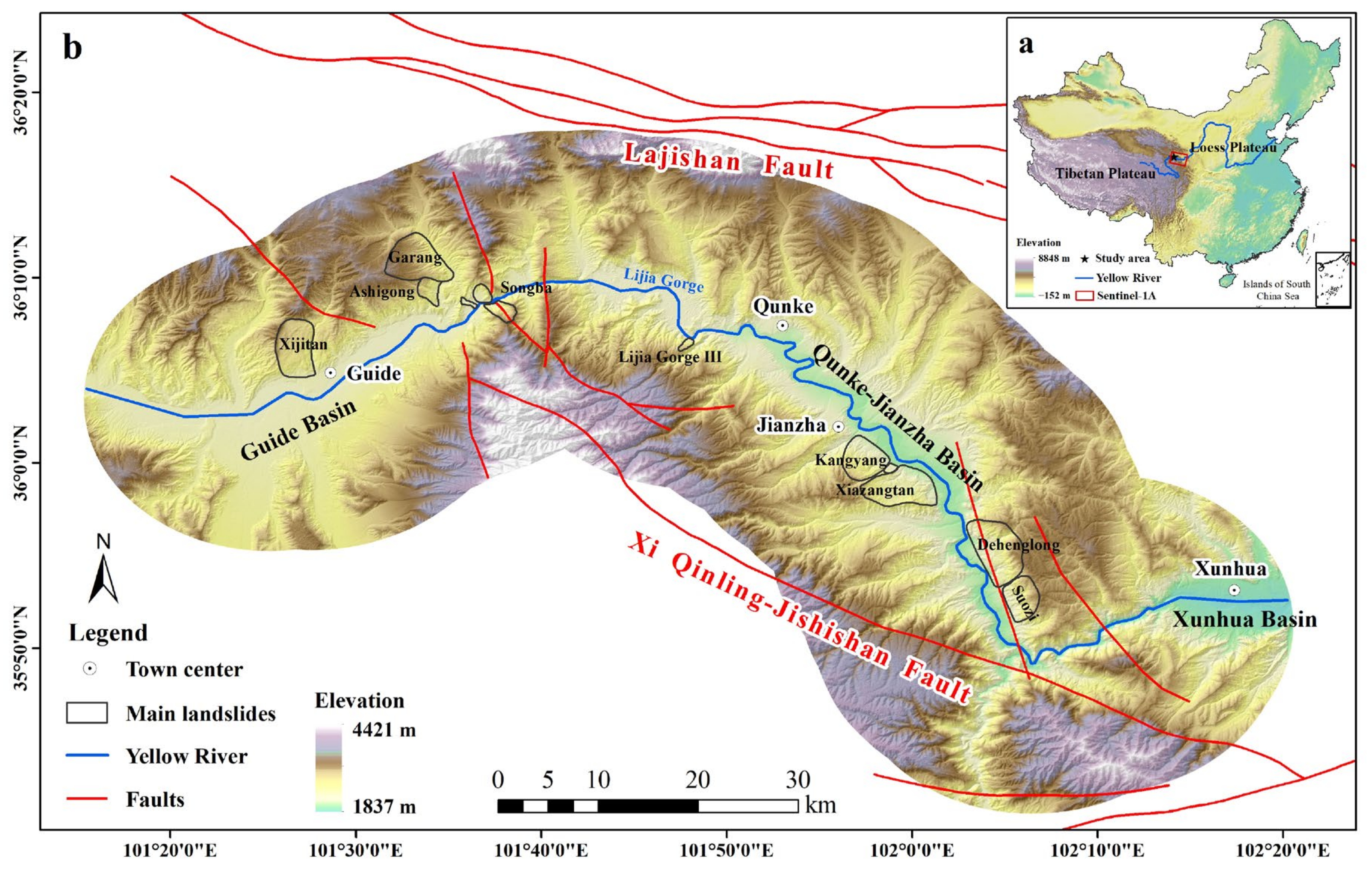
2. Study Area
3. Datasets and Methodology
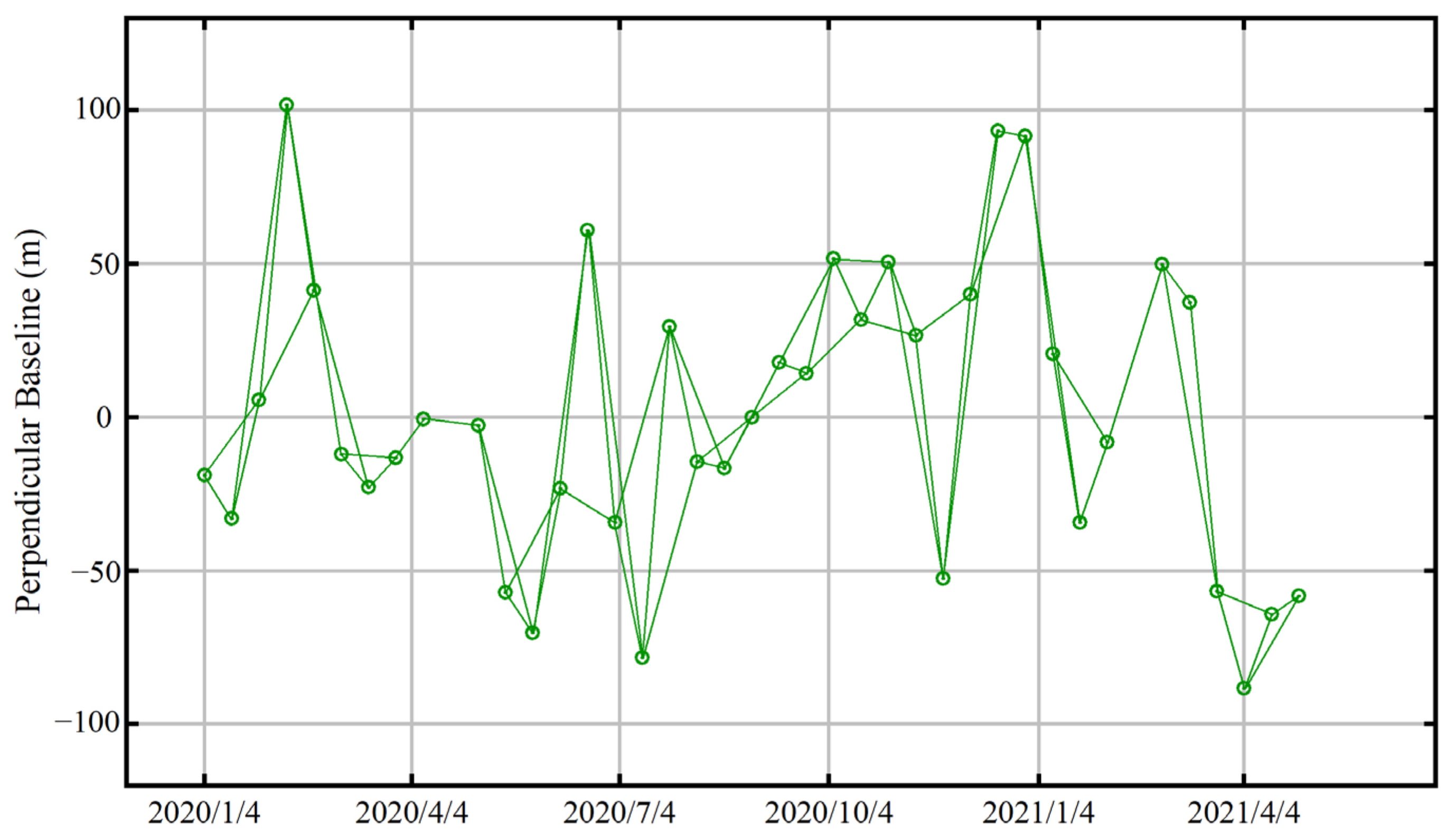
3.1. Data
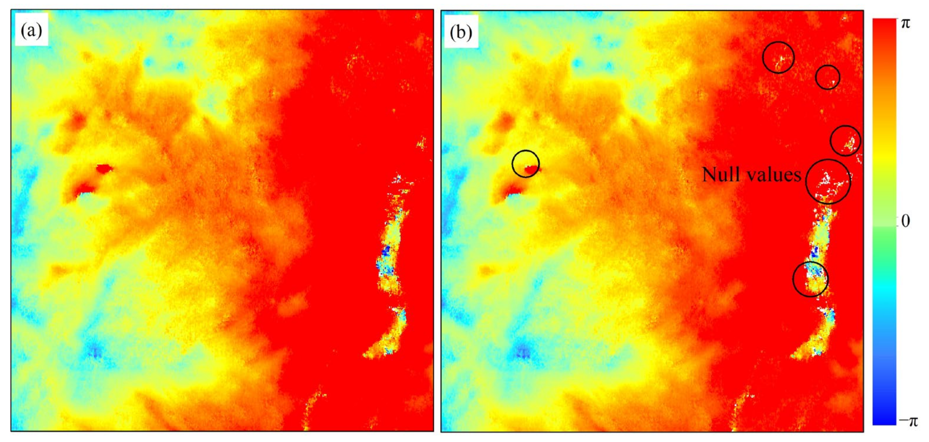
3.2. Interferometric Point Target Analysis (IPTA)
3.3. Hot Spot Analysis
3.4. Semantic Segmentation Models
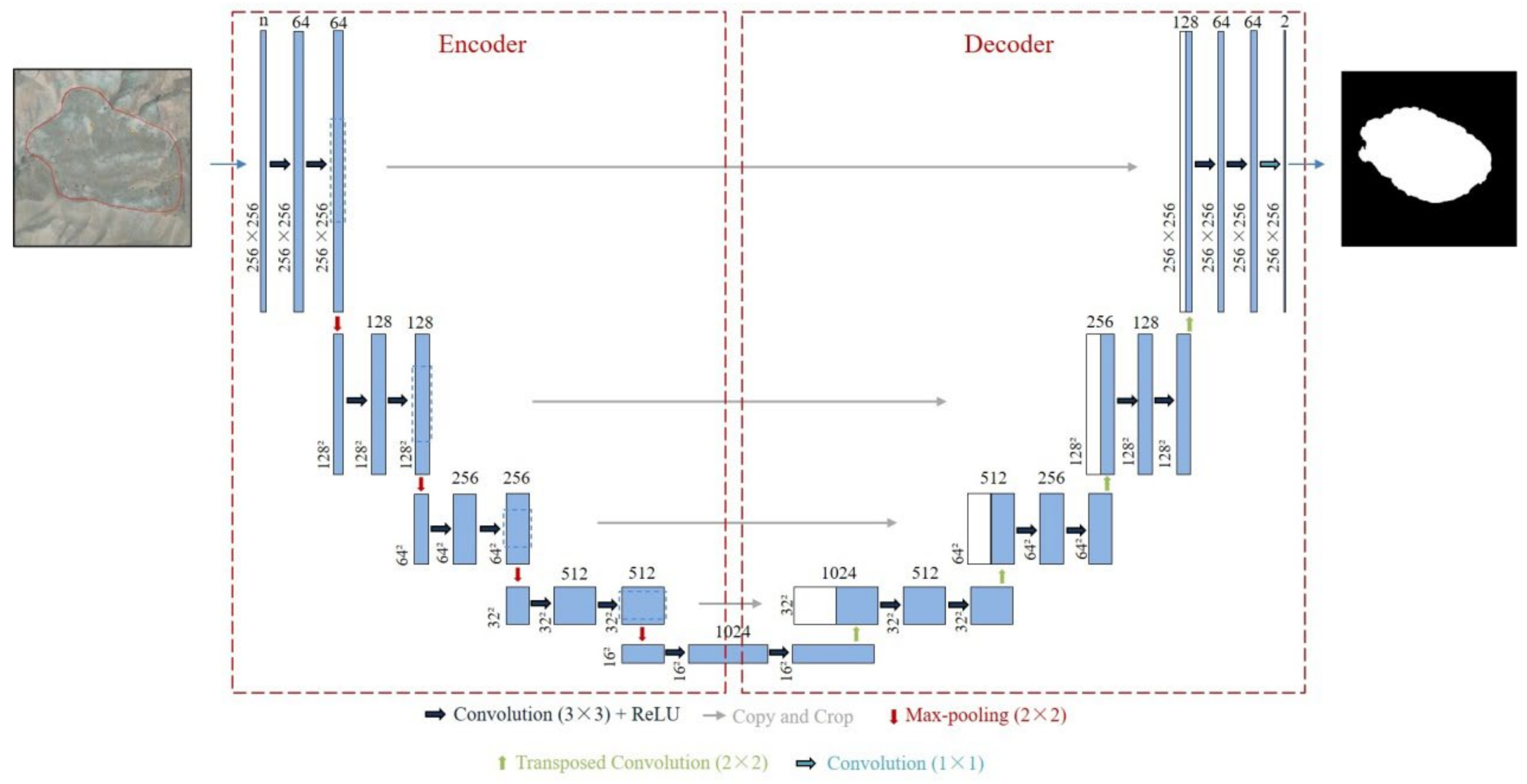
3.4.1. U-Net Model
3.4.2. SegNet Model
3.5. Evaluation Indexes
4. Experiment and Results
4.1. Dataset Preparation
4.1.1. InSAR Deformation
4.1.2. Hot Spot Analysis
4.1.3. Topographic Dataset
4.1.4. Sample Annotation
4.2. Dataset Processing for Model
4.3. Experimental Setup
4.4. Experimental Result
4.4.1. Comparison of Different Deformation Indexes
4.4.2. Topographic Information Addition Identification Model
5. Discussion
5.1. Effects of the Data for Model
5.2. Advantages of the Model
5.3. Limitations and Further Directions of the Model
6. Conclusions
Author Contributions
Funding
Data Availability Statement
Acknowledgments
Conflicts of Interest
References
- Kang, Y.; Lu, Z.; Zhao, C.; Qu, W. Inferring slip-surface geometry and volume of creeping landslides based on InSAR: A case study in Jinsha River basin. Remote Sens. Environ. 2023, 294, 113620. [Google Scholar] [CrossRef]
- Pradhan, B.; Dikshit, A.; Lee, S.; Kim, H. An Explainable AI (XAI) Model for Landslide Susceptibility Modeling. Appl. Soft Comput. 2023, 142, 110324. [Google Scholar] [CrossRef]
- Karagianni, A.; Lazos, I.; Chatzipetros, A. Remote sensing techniques in disaster management: Amynteon mine landslides, Greece. In Intelligent Systems for Crisis Management: Gi4DM 2018; Springer: Cham, Switzerland, 2019; Volume 11, pp. 209–235. [Google Scholar]
- Wasowski, J.; Keefer, D.K.; Lee, C.T. Toward the next generation of research on earthquake-induced landslides: Current issues and future challenges. Eng. Geol. 2011, 122, 1–8. [Google Scholar] [CrossRef]
- Chen, Z.; Huang, Y.; He, X.; Shao, X.; Li, L.; Xu, C.; Wang, S.; Xu, X.; Xiao, Z. Landslides triggered by the 10 June 2022 Maerkang earthquake swarm, Sichuan, China: Spatial distribution and tectonic significance. Landslides 2023, 20, 2155–2169. [Google Scholar] [CrossRef]
- Micu, M.; Micu, D.; Havenith, H.B. Earthquake-induced landslide hazard assessment in the Vrancea Seismic Region (Eastern Carpathians, Romania): Constraints and perspectives. Geomorphology 2023, 427, 108635. [Google Scholar] [CrossRef]
- Naudet, V.; Lazzari, M.; Perrone, A.; Loperte, A.; Piscitelli, S.; Lapenna, V. Integrated geophysical and geomorphological approach to investigate the snowmelt-triggered landslide of Bosco Piccolo village (Basilicata, southern Italy). Eng. Geol. 2008, 98, 156–167. [Google Scholar] [CrossRef]
- Zhang, S.; Fan, Q.; Niu, Y.; Qiu, S.; Si, J.; Feng, Y.; Zhang, S.; Song, Z.; Li, Z. Two-dimensional deformation monitoring for spatiotemporal evolution and failure mode of Lashagou landslide group, Northwest China. Landslides 2023, 20, 447–459. [Google Scholar] [CrossRef]
- Sepúlveda, S.A.; Tobar, C.; Rosales, V.; Ochoa-Cornejo, F.; Lara, M. Megalandslides and deglaciation: Modelling of two case studies in the Central Andes. Nat. Hazards 2023, 118, 1561–1572. [Google Scholar] [CrossRef]
- Donnini, M.; Santangelo, M.; Gariano, S.L.; Bucci, F.; Peruccacci, S.; Alvioli, M.; Althuwaynee, O.; Ardizzone, F.; Bianchi, C.; Bornaetxea, T.; et al. Landslides triggered by an extraordinary rainfall event in Central Italy on September 15, 2022. Landslides 2023, 20, 2199–2211. [Google Scholar] [CrossRef]
- Santangelo, M.; Althuwaynee, O.; Alvioli, M.; Ardizzone, F.; Bianchi, C.; Bornaetxea, T.; Brunetti, M.T.; Bucci, F.; Cardinali, M.; Donnini, M.; et al. Inventory of landslides triggered by an extreme rainfall event in Marche-Umbria, Italy, on 15 September 2022. Sci. Data 2023, 10, 427. [Google Scholar] [CrossRef]
- Aránguiz, R.; Caamaño, D.; Espinoza, M.; Gómez, M.; Maldonado, F.; Sepúlveda, V.; Rogel, I.; Oyarzun, J.C.; Duhart, P. Analysis of the cascading rainfall–landslide–tsunami event of June 29th, 2022, Todos los Santos Lake, Chile. Landslides 2023, 20, 801–811. [Google Scholar] [CrossRef]
- Liu, X.; Zhao, C.; Zhang, Q.; Yang, C.; Zhu, W. Heifangtai loess landslide type and failure mode analysis with ascending and descending Spot-mode TerraSAR-X datasets. Landslides 2020, 17, 205–215. [Google Scholar] [CrossRef]
- Kong, J.; Zhuang, J.; Peng, J.; Ma, P.; Zhan, J.; Mu, J.; Wang, J.; Zhang, D.; Zheng, J.; Fu, Y.; et al. Failure mechanism and movement process of three loess landslides due to freeze-thaw cycle in the Fangtai village, Yongjing County, Chinese Loess Plateau. Eng. Geol. 2023, 315, 107030. [Google Scholar] [CrossRef]
- Dong, Y.; Liao, Z.; Wang, J.; Liu, Q.; Cui, L. Potential failure patterns of a large landslide complex in the Three Gorges Reservoir area. Bull. Eng. Geol. Environ. 2023, 82, 41. [Google Scholar] [CrossRef]
- Zou, Z.; Luo, T.; Zhang, S.; Duan, H.; Li, S.; Wang, J.; Deng, Y.; Wang, J. A novel method to evaluate the time-dependent stability of reservoir landslides: Exemplified by Outang landslide in the Three Gorges Reservoir. Landslides 2023, 20, 1731–1746. [Google Scholar] [CrossRef]
- Kalantar, B.; Ueda, N.; Saeidi, V.; Ahmadi, K.; Halin, A.A.; Shabani, F. Landslide Susceptibility Mapping: Machine and Ensemble Learning Based on Remote Sensing Big Data. Remote Sens. 2020, 12, 1737. [Google Scholar] [CrossRef]
- Liao, M.; Zhang, L.; Shi, X. Methods and Practices of Landslide Deformation Monitoring with SAR; Science Press: Beijing, China, 2017. (In Chinese) [Google Scholar]
- Antonielli, B.; Monserrat, O.; Bonini, M.; Righini, G.; Sani, F.; Luzi, G.; Feyzullayev, A.A.; Aliyev, C.S. Pre-eruptive ground deformation of Azerbaijan mud volcanoes detected through satellite radar interferometry (DInSAR). Tectonophysics 2014, 637, 163–177. [Google Scholar] [CrossRef]
- Wasowski, J.; Bovenga, F. Investigating landslides and unstable slopes with satellite Multi Temporal Interferometry: Current issues and future perspectives. Eng. Geol. 2014, 174, 103–138. [Google Scholar] [CrossRef]
- Bürgmann, R.; Rosen, P.A.; Fielding, E.J. Synthetic aperture radar interferometry to measure Earth’s surface topography and its deformation. Annu. Rev. Earth Planet. Sci. 2000, 28, 169–209. [Google Scholar] [CrossRef]
- Zhang, Y.; Meng, X.; Chen, G.; Qiao, L.; Zeng, R.; Chang, J. Detection of geohazards in the Bailong River Basin using synthetic aperture radar interferometry. Landslides 2016, 13, 1273–1284. [Google Scholar] [CrossRef]
- Su, X.; Zhang, Y.; Meng, X.; Rehman, M.U.; Khalid, Z.; Yue, D. Updating Inventory, Deformation, and Development Characteristics of Landslides in Hunza Valley, NW Karakoram, Pakistan by SBAS-InSAR. Remote Sens. 2022, 14, 4907. [Google Scholar] [CrossRef]
- Liu, X.; Zhao, C.; Zhang, Q.; Lu, Z.; Li, Z.; Yang, C.; Zhu, W.; Liu-zeng, J.; Chen, L.; Liu, C. Integration of Sentinel-1 and ALOS/PALSAR-2 SAR datasets for mapping active landslides along the Jinsha River corridor, China. Eng. Geol. 2021, 284, 106033. [Google Scholar] [CrossRef]
- Chang, M.; Sun, W.; Xu, H.; Tang, L. Identification and deformation analysis of potential landslides after the Jiuzhaigou earthquake by SBAS-InSAR. Environ. Sci. Pollut. Res. 2023, 30, 39093–39106. [Google Scholar] [CrossRef]
- Dai, K.; Feng, Y.; Zhuo, G.; Tie, Y.; Deng, J.; Balz, T.; Li, Z. Applicability Analysis of Potential Landslide Identification by InSAR in Alpine-Canyon Terrain—Case Study on Yalong River. IEEE J. Sel. Top. Appl. Earth Obs. Remote Sens. 2022, 15, 2110–2118. [Google Scholar] [CrossRef]
- He, Y.; Wang, W.; Zhang, L.; Chen, Y.; Chen, Y.; Chen, B.; He, X.; Zhao, Z. An identification method of potential landslide zones using InSAR data and landslide susceptibility. Geomat. Nat. Hazards Risk 2023, 14, 2185120. [Google Scholar] [CrossRef]
- Van Den Eeckhaut, M.; Poesen, J.; Verstraeten, G.; Vanacker, V.; Moeyersons, J.; Nyssen, J.; Van Beek, L.P.H. The Effectiveness of Hillshade Maps and Expert Knowledge in Mapping Old Deep-Seated Landslides. Geomorphology 2005, 67, 351–363. [Google Scholar] [CrossRef]
- Lu, P.; Casagli, N.; Catani, F.; Tofani, V. Persistent Scatterers Interferometry Hotspot and Cluster Analysis (PSI-HCA) for detection of extremely slow-moving landslides. Int. J. Remote Sens. 2012, 33, 466–489. [Google Scholar] [CrossRef]
- Zhang, J.; Zhu, W.; Cheng, Y.; Li, Z. Landslide Detection in the Linzhi–Ya’an Section along the Sichuan–Tibet Railway Based on InSAR and Hot Spot Analysis Methods. Remote Sens. 2021, 13, 3566. [Google Scholar] [CrossRef]
- Xun, Z.; Zhao, C.; Kang, Y.; Liu, X.; Liu, Y.; Du, C. Automatic Extraction of Potential Landslides by Integrating an Optical Remote Sensing Image with an InSAR-Derived Deformation Map. Remote Sens. 2022, 14, 2669. [Google Scholar] [CrossRef]
- Saba, S.B.; Ali, M.; Turab, S.A.; Waseem, M.; Faisal, S. Comparison of pixel, sub-pixel and object-based image analysis techniques for co-seismic landslides detection in seismically active area in Lesser Himalaya, Pakistan. Nat. Hazards 2023, 115, 2383–2398. [Google Scholar] [CrossRef]
- Ghorbanzadeh, O.; Gholamnia, K.; Ghamisi, P. The application of ResU-net and OBIA for landslide detection from multi-temporal sentinel-2 images. Big Earth Data 2022, 1–26. [Google Scholar] [CrossRef]
- Blaschke, T. Object Based Image Analysis for Remote Sensing. ISPRS J. Photogramm. Remote Sens. 2010, 65, 2–16. [Google Scholar] [CrossRef]
- Ye, Z.; Yang, K.; Lin, Y.; Guo, S.; Sun, Y.; Chen, X.; Lai, R.; Zhang, H. A comparison between Pixel-based deep learning and Object-based image analysis (OBIA) for individual detection of cabbage plants based on UAV Visible-light images. Comput. Electron. Agric. 2023, 209, 107822. [Google Scholar] [CrossRef]
- Chen, X.; Yao, X.; Zhou, Z.; Liu, Y.; Yao, C.; Ren, K. DRs-UNet: A Deep Semantic Segmentation Network for the Recognition of Active Landslides from InSAR Imagery in the Three Rivers Region of the Qinghai–Tibet Plateau. Remote Sens. 2022, 14, 1848. [Google Scholar] [CrossRef]
- Lateef, F.; Ruichek, Y. Survey on semantic segmentation using deep learning techniques. Neurocomputing 2019, 338, 321–348. [Google Scholar] [CrossRef]
- Wu, Z.; Ma, P.; Zheng, Y.; Gu, F.; Liu, L.; Lin, H. Automatic detection and classification of land subsidence in deltaic metropolitan areas using distributed scatterer InSAR and Oriented R-CNN. Remote Sens. Environ. 2023, 290, 113545. [Google Scholar] [CrossRef]
- Wang, Z.; Sun, T.; Hu, K.; Zhang, Y.; Yu, X.; Li, Y. A Deep Learning Semantic Segmentation Method for Landslide Scene Based on Transformer Architecture. Sustainability 2022, 14, 16311. [Google Scholar] [CrossRef]
- Li, H.; He, Y.; Xu, Q.; Deng, J.; Li, W.; Wei, Y.; Zhou, J. Sematic segmentation of loess landslides with STAPLE mask and fully connected conditional random field. Landslides 2023, 20, 367–380. [Google Scholar] [CrossRef]
- Yu, B.; Chen, F.; Xu, C. Landslide detection based on contour-based deep learning framework in case of national scale of Nepal in 2015. Comput. Geosci. 2020, 135, 104388. [Google Scholar] [CrossRef]
- Liu, Y.; Yao, X.; Gu, Z.; Zhou, Z.; Liu, X.; Chen, X.; Wei, S. Study of the Automatic Recognition of Landslides by Using InSAR Images and the Improved Mask R-CNN Model in the Eastern Tibet Plateau. Remote Sens. 2022, 14, 3362. [Google Scholar] [CrossRef]
- Liu, P.; Wei, Y.; Wang, Q.; Chen, Y.; Xie, J. Research on Post-Earthquake Landslide Extraction Algorithm Based on Improved U-Net Model. Remote Sens. 2020, 12, 894. [Google Scholar] [CrossRef]
- LeCun, Y.; Bengio, Y.; Hinton, G. Deep learning. Nature 2015, 521, 436–444. [Google Scholar] [CrossRef]
- Zhang, T.; Zhang, W.; Cao, D.; Yi, Y.; Wu, X. A New Deep Learning Neural Network Model for the Identification of InSAR Anomalous Deformation Areas. Remote Sens. 2022, 14, 2690. [Google Scholar] [CrossRef]
- Guo, H.; Yi, B.; Yao, Q.; Gao, P.; Li, H.; Sun, J.; Zhong, C. Identification of Landslides in Mountainous Area with the Combination of SBAS-InSAR and Yolo Model. Sensors 2022, 22, 6235. [Google Scholar] [CrossRef]
- Niu, C.; Yin, W.; Xue, W.; Sui, Y.; Xun, X.; Zhou, X.; Zhang, S.; Xue, Y. Multi-Window Identification of Landslide Hazards Based on InSAR Technology and Factors Predisposing to Disasters. Land 2023, 12, 173. [Google Scholar] [CrossRef]
- Peng, J.; Ma, R.; Lu, Q.; Li, X.; Shao, T. Geological hazards effects of uplift of Qinghai-Tibet Plateau. Adv. Earth Sci. 2004, 19, 457–466. (In Chinese) [Google Scholar]
- Yin, Z.; Qin, X.; Zhao, X.; Li, X.; Cheng, G.; Wei, G.; Shi, L.; Yuan, C. Temporal and Spatial Evolution and Triggering Mechanism of Landslide and Debris Flow in the Upper Reaches of the Yellow River; Science Press: Beijing, China, 2016. (In Chinese) [Google Scholar]
- Shi, X.; Yang, C.; Zhang, L.; Jiang, H.; Liao, M.; Zhang, L.; Liu, X. Mapping and characterizing displacements of active loess slopes along the upstream Yellow River with multi-temporal InSAR datasets. Sci. Total Environ. 2019, 674, 200–210. [Google Scholar] [CrossRef] [PubMed]
- Li, J. The environmental effects of the uplift of the Qinghai-Xizang Plateau. Quat. Sci. Rev. 1991, 10, 479–483. [Google Scholar]
- Craddock, W.H.; Kirby, E.; Harkins, N.W.; Zhang, H.; Shi, X.; Liu, J. Rapid fluvial incision along the Yellow River during headward basin integration. Nat. Geosci. 2010, 3, 209–213. [Google Scholar] [CrossRef]
- Guo, X.; Wei, J.; Lu, Y.; Song, Z.; Liu, H. Geomorphic Effects of a Dammed Pleistocene Lake Formed by Landslides along the Upper Yellow River. Water 2020, 12, 1350. [Google Scholar] [CrossRef]
- Yin, Z.; Qin, X.; Zhao, W.; Wei, G. Characteristics of landslides in upper reaches of Yellow River with multiple data of remote sensing. J. Eng. Geol. 2013, 21, 779–787. (In Chinese) [Google Scholar]
- Guo, X.; Sun, Z.; Lai, Z.; Lu, Y.; Li, X. Optical dating of landslide-dammed lake deposits in the upper Yellow River, Qinghai-Tibetan Plateau, China. Quat. Int. 2016, 392, 233–238. [Google Scholar] [CrossRef]
- Qin, X.; Yin, Z.; Zhao, W. Xijitan landslide in guide basin in the upper reaches of the Yellow River and its Dammed Lakes. Geophys. Remote Sens. 2015, 4, 147. [Google Scholar]
- Shi, X.; Zhang, L.; Tang, M.; Li, M.; Liao, M. Investigating a reservoir bank slope displacement history with multi-frequency satellite SAR data. Landslides 2017, 14, 1961–1973. [Google Scholar] [CrossRef]
- Hooper, A. A multi-temporal InSAR method incorporating both persistent scatterer and small baseline approaches. Geophys. Res. Lett. 2008, 35, 96–106. [Google Scholar] [CrossRef]
- Werner, C.; Wegmuller, U.; Strozzi, T.; Wiesmann, A. Interferometric point target analysis for deformation mapping. IEEE Geosci. Remote Sens. Soci. 2003, 7, 4362–4364. [Google Scholar]
- Liu, H.; Zhou, B.; Bai, Z.; Zhao, W.; Zhu, M.; Zheng, K.; Yang, S.; Li, G. Applicability Assessment of Multi-Source DEM-Assisted InSAR Deformation Monitoring Considering Two Topographical Features. Land 2023, 12, 1284. [Google Scholar] [CrossRef]
- Alaska Satellite Facility—Distributed Active Archive Center. Available online: https://asf.alaska.edu/data-sets/derived-data-sets/alos-palsar-rtc/alos-palsar-radiometric-terrain-correction/ (accessed on 17 October 2023).
- Solari, L.; Soldato, M.; Montalti, R.; Bianchini, S.; Raspini, F.; Thuegaz, P.; Bertolo, D.; Tofani, V.; Casagli, N. A Sentinel-1 based hot-spot analysis: Landslide mapping in north-western Italy. Int. J. Remote Sens. 2019, 40, 7898–7921. [Google Scholar] [CrossRef]
- Zhu, K.; Xu, P.; Cao, C.; Zheng, L.; Liu, Y.; Dong, X. Preliminary identification of geological hazards from Songpinggou to Feihong in Mao County along the Minjiang River using SBAS-InSAR technique integrated multiple spatial analysis methods. Sustainability 2021, 13, 1017. [Google Scholar] [CrossRef]
- Lu, P.; Bai, S.; Tofani, V.; Casagli, N. Landslides detection through optimized hot spot analysis on persistent scatterers and distributed scatterers. ISPRS J. Photogramm. Remote Sens. 2019, 156, 147–159. [Google Scholar] [CrossRef]
- Ord, J.; Getis, A. Local spatial autocorrelation statistics: Distributional issues and an application. Geogr. Anal. 2015, 27, 286–306. [Google Scholar] [CrossRef]
- Getis, A.; Ord, J. The analysis of spatial association by use of distance statistics. Geogr. Anal. 1992, 24, 189–206. [Google Scholar] [CrossRef]
- Lu, P.; Catani, F.; Tofani, V.; Casagli, N. Quantitative hazard and risk assessment for slow-moving landslides from Persistent Scatterer Interferometry. Landslides 2014, 11, 685–696. [Google Scholar] [CrossRef]
- Silverman, B.W. Density Estimation for Statistics and Data Analysis; Routledge: New York, NY, USA, 1986. [Google Scholar]
- Ronneberger, O.; Fischer, P.; Brox, T. U-net: Convolutional networks for biomedical image segmentation. In Proceedings of the Medical Image Computing and Computer-Assisted Intervention—MICCAI, Munich, Germany, 5–9 October 2015; pp. 234–241. [Google Scholar]
- Bhuyan, K.; Meena, S.R.; Nava, L.; Westen, C.V.; Floris, M.; Catani, F. Mapping landslides through a temporal lens: An insight toward multi-temporal landslide mapping using the u-net deep learning model. GISci. Remote Sens. 2023, 60, 2182057. [Google Scholar] [CrossRef]
- Chen, H.; He, Y.; Zhang, L.; Yao, S.; Yang, W.; Fang, Y.; Liu, Y.; Gao, B. A landslide extraction method of channel attention mechanism U-Net network based on Sentinel-2A remote sensing images. Int. J. Digit. Earth 2023, 16, 552–577. [Google Scholar] [CrossRef]
- Bragagnolo, L.; Rezende, L.R.; da Silva, R.V.; Grzybowski, J.M.V. Convolutional neural networks applied to semantic segmentation of landslide scars. Catena 2021, 201, 105189. [Google Scholar] [CrossRef]
- Meena, S.R.; Soares, L.P.; Grohmann, C.H.; Westen, C.V.; Bhuyan, K.; Singh, R.P.; Floris, M.; Catani, F. Landslide detection in the Himalayas using machine learning algorithms and U-Net. Landslides 2022, 19, 1209–1229. [Google Scholar] [CrossRef]
- Badrinarayanan, V.; Kendall, A.; Cipolla, R. Segnet: A deep convolutional encoder-decoder architecture for image segmentation. IEEE Trans. Pattern Anal. Mach. Intell. 2017, 39, 2481–2495. [Google Scholar] [CrossRef]
- Kolhar, S.; Jagtap, J. Convolutional neural network based encoder-decoder architectures for semantic segmentation of plants. Ecol. Inform. 2021, 64, 101373. [Google Scholar] [CrossRef]
- Antara, I.M.O.G.; Shimizu, N.; Osawa, T.; Nusrsa, I.W. An application of SegNet for detecting landslide areas by using fully polarimetric SAR data. Ecotrophic 2019, 13, 215–226. [Google Scholar] [CrossRef]
- Manickam, R.; Kumar Rajan, S.; Subramanian, C.; Xavi, A.; Julie Eanoch, G.; Robinson Yesudhas, H. Person identification with aerial imaginary using SegNet based semantic segmentation. Earth Sci. Inform. 2020, 13, 1293–1304. [Google Scholar] [CrossRef]
- Chollet, F. Deep Learning with Python; Manning: Greenwich, CT, USA, 2021. [Google Scholar]
- Hacıefendioğlu, K.; Demir, G.; Başağa, H.B. Landslide detection using visualization techniques for deep convolutional neural network models. Nat. Hazards 2021, 109, 329–350. [Google Scholar] [CrossRef]
- Hanssen, R.F. Satellite radar interferometry for deformation monitoring: A priori assessment of feasibility and accuracy. Int. J. Appl. Earth Obs. Geoinf. 2005, 6, 253–260. [Google Scholar] [CrossRef]
- Colesanti, C.; Wasowski, J. Satellite SAR interferometry for wide-area slope hazard detection and site-specific monitoring of slow landslides. In Proceedings of the Ninth International Symposium on Landslides, Rio de Janeiro, Brazil, 28 June–2 July 2004; pp. 795–802. [Google Scholar]
- Du, P.; Xu, Y.; Tian, Q.; Li, W. Using Google Earth images to extract dense landslides induced by historical earthquakes at the Southwest of Ordos, China. Front. Earth Sci. 2021, 8, 633342. [Google Scholar]
- Singhroy, V. Satellite remote sensing applications for landslide detection and monitoring. In Landslides–Disaster Risk Reduction; Springer: Berlin/Heidelberg, Germany, 2009; pp. 143–158. [Google Scholar]
- Guzzetti, F.; Mondini, A.C.; Cardinali, M.; Fiorucci, F.; Santangelo, M.; Chang, K.T. Landslide inventory maps: New tools for an old problem. Earth-Sci. Rev. 2012, 112, 42–66. [Google Scholar] [CrossRef]
- Xu, G.; Wang, Y.; Wang, L.; Soares, L.P.; Grohmann, C.H. Feature-based constraint deep CNN method for mapping rainfall-induced landslides in remote regions with mountainous terrain: An application to Brazil. IEEE J. Sel. Top. Appl. Earth Obs. Remote Sens. 2022, 15, 2644–2659. [Google Scholar] [CrossRef]
- Konečný, J.; Liu, J.; Richtárik, P.; Takáč, M. Mini-batch semi-stochastic gradient descent in the proximal setting. IEEE J. Sel. Top. Signal Process. 2015, 10, 242–255. [Google Scholar] [CrossRef]
- Du, B.; Zhao, Z.; Hu, X.; Wu, G.; Han, L.; Sun, L.; Gao, Q. Landslide susceptibility prediction based on image semantic segmentation. Comput. Geosci. 2021, 155, 104860. [Google Scholar] [CrossRef]
- Wan, H.; Zeng, X.; Fan, Z.; Zhang, S.; Kang, M. U2ESPNet—A lightweight and high-accuracy convolutional neural network for real-time semantic segmentation of visible branches. Comput. Electron. Agric. 2023, 204, 107542. [Google Scholar] [CrossRef]
- Ji, S.; Yu, D.; Shen, C.; Li, W.; Xu, Q. Landslide detection from an open satellite imagery and digital elevation model dataset using attention boosted convolutional neural networks. Landslides 2020, 17, 1337–1352. [Google Scholar] [CrossRef]
- Wang, X.; Jing, S.; Dai, H.; Shi, A. High-resolution remote sensing images semantic segmentation using improved UNet and SegNet. Comput. Electr. Eng. 2023, 108, 108734. [Google Scholar] [CrossRef]
- Wang, K.; Zhang, S.; DelgadoTéllez, R.; Wei, F. A new slope unit extraction method for regional landslide analysis based on morphological image analysis. Bull. Eng. Geol. Environ. 2019, 78, 4139–4151. [Google Scholar] [CrossRef]
- Huang, F.; Tao, S.; Chang, Z.; Huang, J.; Fan, X.; Jiang, S.; Li, W. Efficient and automatic extraction of slope units based on multi-scale segmentation method for landslide assessments. Landslides 2021, 18, 3715–3731. [Google Scholar] [CrossRef]
- Chen, Z.; Liang, S.; Ke, Y.; Yang, Z.; Zhao, H. Landslide susceptibility assessment using different slope units based on the evidential belief function model. Geocarto Int. 2020, 35, 1641–1664. [Google Scholar] [CrossRef]
- Hansen, A. Landslide hazard analysis. In Slope Instability; Brunsden, D., Prior, E., Eds.; Wiley: New York, NY, USA, 1984; pp. 523–602. [Google Scholar]
- Li, Y.; Zhang, Y.; Meng, X.; Su, X.; Liu, W.; Wang, A.; Guo, F.; Liang, Y. Deformation process and kinematic evolution of the large Daxiaowan earthflow in the NE Qinghai-Tibet Plateau. Eng. Geol. 2023, 316, 107062. [Google Scholar] [CrossRef]
- Amatya, P.; Kirschbaum, D.; Stanley, T.; Tanyas, H. Landslide mapping using object-based image analysis and open source tools. Eng. Geol. 2021, 282, 106000. [Google Scholar] [CrossRef]
- Šiljeg, A.; Panđa, L.; Domazetović, F.; Marić, I.; Gašparović, M.; Borisov, M.; Milošević, R. Comparative Assessment of Pixel and Object-Based Approaches for Mapping of Olive Tree Crowns Based on UAV Multispectral Imagery. Remote Sens. 2022, 14, 757. [Google Scholar] [CrossRef]
- Hou, F.; Lei, W.; Li, S.; Xi, J.; Xu, M.; Luo, J. Improved Mask R-CNN with distance guided intersection over union for GPR signature detection and segmentation. Autom. Constr. 2021, 121, 103414. [Google Scholar] [CrossRef]
- Ghorbanzadeh, O.; Shahabi, H.; Crivellari, A.; Homayouni, S.; Blaschke, T.; Ghamisi, P. Landslide detection using deep learning and object-based image analysis. Landslides 2022, 19, 929–939. [Google Scholar] [CrossRef]
- Dong, J.; Zhang, L.; Liao, M.; Gong, J. Improved correction of seasonal tropospheric delay in InSAR observations for landslide deformation monitoring. Remote Sens. Environ. 2019, 233, 111370. [Google Scholar] [CrossRef]
- Wasowski, J.; Bovenga, F. Remote sensing of landslide motion with emphasis on satellite multi-temporal interferometry applications: An overview. In Landslide Hazards, Risks, and Disasters; Elsevier: Amsterdam, The Netherlands, 2022; pp. 365–438. [Google Scholar]
- Amankwah, S.O.Y.; Wang, G.; Gnyawali, K.; Hagan, D.F.T.; Sarfo, I.; Zhen, D.; Nooni, I.K.; Ullah, W.; Duan, Z. Landslide detection from bitemporal satellite imagery using attention-based deep neural networks. Landslides 2022, 19, 2459–2471. [Google Scholar] [CrossRef]
- Yang, S.; Wang, Y.; Wang, P.; Mu, J.; Jiao, S.; Zhao, X.; Wang, Z.; Wang, K.; Zhu, Y. Automatic Identification of Landslides Based on Deep Learning. Appl. Sci. 2022, 12, 8153. [Google Scholar] [CrossRef]


| Num | Model | Data | Precision | Recall | F1 Score | IoU |
|---|---|---|---|---|---|---|
| I | SegNet | Google Earth Image (RGB) + InSAR Deformation Points | 0.879 | 0.719 | 0.785 | 0.652 |
| II | Google Earth Image (RGB) + Hot Spot Map | 0.853 | 0.779 | 0.809 | 0.686 | |
| III | U-Net | Google Earth Image (RGB) + InSAR Deformation Points | 0.843 | 0.775 | 0.806 | 0.676 |
| IV | Google Earth Image (RGB) + Hot Spot Map | 0.829 | 0.807 | 0.812 | 0.689 |
| Num | Model | Data | Precision | Recall | F1 Score | IoU |
|---|---|---|---|---|---|---|
| V | SegNet | Google Earth Image (RGB) + Hot Spot Map + Slope | 0.797 | 0.836 | 0.811 | 0.688 |
| VI | Google Earth Image (RGB) + Hot Spot Map + Aspect | 0.816 | 0.833 | 0.819 | 0.7 | |
| VII | Google Earth Image (RGB) + Hot Spot Map + Elevation | 0.847 | 0.758 | 0.794 | 0.666 | |
| VIII | Google Earth Image (RGB) + Hot Spot Map + Slope + Aspect | 0.806 | 0.839 | 0.817 | 0.696 | |
| IX | Google Earth Image (RGB) + Hot Spot Map + Slope + Elevation | 0.82 | 0.814 | 0.811 | 0.689 | |
| X | Google Earth Image (RGB) + Hot Spot Map + Aspect + Elevation | 0.828 | 0.797 | 0.806 | 0.682 | |
| XI | Google Earth Image (RGB) + Hot Spot Map + Slope + Aspect + Elevation | 0.846 | 0.78 | 0.806 | 0.682 | |
| XII | U-Net | Google Earth Image (RGB) + Hot Spot Map + Slope | 0.828 | 0.812 | 0.814 | 0.693 |
| XIII | Google Earth Image (RGB) + Hot Spot Map + Aspect | 0.822 | 0.835 | 0.823 | 0.705 | |
| XIV | Google Earth Image (RGB) + Hot Spot Map + Elevation | 0.773 | 0.823 | 0.792 | 0.662 | |
| XV | Google Earth Image (RGB) + Hot Spot Map + Slope + Aspect | 0.81 | 0.836 | 0.818 | 0.697 | |
| XVI | Google Earth Image (RGB) + Hot Spot Map + Slope + Elevation | 0.858 | 0.765 | 0.803 | 0.678 | |
| XVII | Google Earth Image (RGB) + Hot Spot Map + Aspect + Elevation | 0.849 | 0.786 | 0.811 | 0.688 | |
| XVIII | Google Earth Image (RGB) + Hot Spot Map + Slope + Aspect + Elevation | 0.811 | 0.836 | 0.818 | 0.698 |
Disclaimer/Publisher’s Note: The statements, opinions and data contained in all publications are solely those of the individual author(s) and contributor(s) and not of MDPI and/or the editor(s). MDPI and/or the editor(s) disclaim responsibility for any injury to people or property resulting from any ideas, methods, instructions or products referred to in the content. |
© 2023 by the authors. Licensee MDPI, Basel, Switzerland. This article is an open access article distributed under the terms and conditions of the Creative Commons Attribution (CC BY) license (https://creativecommons.org/licenses/by/4.0/).
Share and Cite
Liang, Y.; Zhang, Y.; Li, Y.; Xiong, J. Automatic Identification for the Boundaries of InSAR Anomalous Deformation Areas Based on Semantic Segmentation Model. Remote Sens. 2023, 15, 5262. https://doi.org/10.3390/rs15215262
Liang Y, Zhang Y, Li Y, Xiong J. Automatic Identification for the Boundaries of InSAR Anomalous Deformation Areas Based on Semantic Segmentation Model. Remote Sensing. 2023; 15(21):5262. https://doi.org/10.3390/rs15215262
Chicago/Turabian StyleLiang, Yiwen, Yi Zhang, Yuanxi Li, and Jiaqi Xiong. 2023. "Automatic Identification for the Boundaries of InSAR Anomalous Deformation Areas Based on Semantic Segmentation Model" Remote Sensing 15, no. 21: 5262. https://doi.org/10.3390/rs15215262