Vision Transformer-Based Ensemble Learning for Hyperspectral Image Classification

Abstract

Hyperspectral image (HSI) classification, due to its characteristic combination of images and spectra, has important applications in various fields through pixel-level image classification. The fusion of spatial–spectral features is a topic of great interest in the context of hyperspectral image classification, which typically requires selecting a larger spatial neighborhood window, potentially leading to overlaps between training and testing samples. Vision Transformer (ViTs), with their powerful global modeling abilities, have had a significant impact in the field of computer vision through various variants. In this study, an ensemble learning framework for HSI classification is proposed by integrating multiple variants of ViTs, achieving high-precision pixel-level classification. Firstly, the spatial shuffle operation was introduced to preprocess the training samples for HSI classification. By randomly shuffling operations using smaller spatial neighborhood windows, a greater potential spatial distribution of pixels can be described. Then, the training samples were transformed from a 3D cube to a 2D image, and a learning framework was built by integrating seven ViT variants. Finally, a two-level ensemble strategy was employed to achieve pixel-level classification based on the results of multiple ViT variants. Our experimental results demonstrate that the proposed ensemble learning framework achieves stable and significantly high classification accuracy on multiple publicly available HSI datasets. The proposed method also shows notable classification performance with varying numbers of training samples. Moreover, herein, it is proven that the spatial shuffle operation plays a crucial role in improving classification accuracy. By introducing superior individual classifiers, the proposed ensemble framework is expected to achieve even better classification performance.

1. Introduction

Remote sensing, with its advantages of wide observation ranges, short time cycles, and dynamic tracking, has become the primary means of Earth observation. Hyperspectral remote sensing technology, as an organic combination of spectral and imaging techniques, uses imaging spectrometers to measure radiation intensity within a wide spectral range for specific scenes, generating a data cube that combines one-dimensional spectral responses with two-dimensional spatial information. This enables the synchronous acquisition of geometric, radiometric, and spectral information pertaining to target objects. Compared to traditional remote sensing, hyperspectral remote sensing provides more abundant spectral–spatial information, greatly promoting the transition from qualitative analysis to quantitative analysis in remote sensing [1]. The spectral fusion characteristic of hyperspectral image (HSI) data gives it prominent advantages in the fine classification and identification of land cover, making it widely applied in fields such as geological survey [2], precision agriculture [3], forest inventory [4], environmental monitoring [5], biomedical research [6], and more.

HSI data has the advantage of high spectral resolution, allowing it to capture delicate spectral characteristics of the interested target. This has made land cover classification a popular research direction in the field of HSI analysis [7]. Considering the high-dimensional nature of HSI samples, researchers have applied various machine learning methods to HSI classification over the past few decades, including logistic regression [8], Support Vector Machines (SVM) [9], Sparse Representation [10], Random Forest (RF) [11], and Decision Trees [12]. However, due to the limited number of available training samples regarding HSI data, which often cannot satisfy the requirements of the spectral dimension, these classifiers still exhibit inadequate classification performance on the original data [13]. Additionally, the high-spectral-resolution HSI data inevitably contain a certain amount of redundant information between adjacent spectral bands [14], and the original spectral features are often not the most effective representation for distinguishing the target of interest.

To address the aforementioned problems, HSI feature extraction methods have emerged. The purpose of these methods is to explore discriminative information of different objects in order to enable more accurate category prediction in the feature space via the use of classifiers. Early feature extraction methods include singular spectrum analysis (SSA) [15], principal component analysis (PCA) [16], linear discriminant analysis (LDA) [17], and independent component analysis (ICA) [18], which primarily extract features by learning linear combinations of independent pixels. However, these methods often lack the consideration of spatial contextual information, leading to issues such as outliers and pixel-level misclassification in the resulting classification maps, seriously affecting the reliability of the results. As a result, more research studies have focused on how to extract effective spatial information and integrate it with spectral information for classification tasks [19]. Ref. [20] leverages the advantages of edge-preserving filters (EPF) in extracting image spatial structures by adjusting the parameters of the filters to obtain hyperspectral image spatial information at different scales. In [21], HSI data were treated as a complete tensor, and a three-dimensional discrete wavelet transform was designed to decompose the data into geometric and statistical spatial structures.

The deep learning techniques in HSI classification have received widespread attention in recent years. Researchers have proposed deep learning-based multiscale spatial–spectral classification methods. Compared to traditional methods, deep neural networks have the advantage of extracting high-level nonlinear features from images [22]. In a study by Liang et al., the VGG16 network was used to extract spatial information at different levels of HSI as spatial features at different scales [23]. Wang et. al designed multiscale feature extraction sub-networks for the spectral and spatial information of HSI data. They proposed an adaptive spectral and spatial feature combination method, achieving the collaborative classification of spectral information [24]. A model combining a Convolutional Neural Network (CNN) and Recurrent Neural Network (RNN) was proposed to enhance the discriminative ability of spectral features in [25]. A deep 1D CNN model, which takes pixel vectors as input data and performs classification on hyperspectral data only in the spectral dimension, achieved outstanding accuracy surpassing traditional SVM classifiers [26]. Wan et al. introduced a Graph Convolutional Network (GCN) to overcome the issue of traditional CNN models’ inability to adapt to the distribution and geometric shapes of different objects. They constructed multiple input graphs with different neighborhood scales to achieve multiscale classification [27].

The Vision Transformer (ViT) [28] is the first transformer network for the visual domain. The network treats image patches as inputs and maps them into features that are integrated into the ViT model. Following the emergence of ViTs, many studies have aimed to incorporate transformers such as IPT [29], PVT [30], and the Swin Transformer [31] into image processing. Wang et al. combined K-nearest neighbor attention to utilize the local features of image patches and suppressed redundant information by only considering a subset of attention weights with the highest similarity [32]. Mou et al. designed a spectral attention module that applies different attention weights to guide the network to focus on discriminative spectral information through a gating mechanism [33]. Refiner explored the potential of attention expansion in high-dimensional space and enhanced the local structural characteristics of attention maps using convolutional operations [34]. Zhu et al. studied the attention mechanism in spectral and spatial information and proposed the Residual Spectral–Spatial Attention (RSSAN) mechanism [35], which selectively captures useful features in the spectral and spatial dimensions to improve hyperspectral classification. He et al. introduced a bidirectional encoder representation from a transformer (BERT) model [36], and a new feature channel-based attention calculation method which improves the processing efficiency of high-resolution images compared to existing token-based attention calculation methods was also proposed [37]. Hong et al. proposed SpectralFormer [38], which captures local spectral sequence knowledge from neighboring spectral bands through pixel- or patch-wise inputs. Zhong et al. introduced a spectral-spatial transformer network, which includes a spatial attention module and a spectral correlation module [39]. Some new transformer-based architectures [40,41,42,43,44,45,46] were employed in HSI classification fields and achieved good performance.

In all supervised learning algorithms, the ultimate goal is to train a model that performs well in all aspects and remains stable. However, achieving such ideal results is often challenging. In many cases, only multiple models that excel in certain aspects can be trained (known as weakly supervised models). Ensemble learning aims to combine these weakly supervised models to create a more robust and accurate strongly supervised model. The fundamental idea behind ensemble learning is that by fusing predictions from diverse weak classifiers, errors made by one classifier can be corrected by others, ultimately improving overall performance. Typically, we test new data using a well-converged network to achieve good prediction results. However, in the case of HSI classification, when training samples are limited, a single classification network may perform poorly. Continuously improving the model structure and introducing more feature extraction modules can enhance the network’s feature extraction ability, which can theoretically continuously improve classification accuracy. However, this approach requires more data and greater algorithm requirements, meaning that it is more costly. The advantage of ensemble learning lies in its fewer requirements for each participating algorithm. By designing different ensemble strategies, it often achieves unexpectedly good classification accuracy, so it has a wide range of practical applications. Therefore, this paper adopts an ensemble learning approach using a two-level ensemble strategy to combine the outcomes of several single-classification networks based on ViT. Due to their different architectural designs, each ViT model has different feature extraction capabilities and can extract features for classification from multiple different aspects, which ensures that each basic ViT classifier has a large degree of diversity. Hence, the proposed approach yields stable and high-performing classification maps for HSI classification.

The main contributions of this paper are as follows:

• Proposed an ensemble learning framework based on ViT that combines the classification performance of multiple ViT models using two levels of ensemble strategies. The two ensemble strategies consistently achieve higher classification accuracy compared to individual ViT methods.
• Introduced the spatial shuffle pre-processing technique, which converts the three-dimensional cubic data into two-dimensional images for processing, making it more suitable for the ViT architecture.
• With the two-level ensemble strategies, there is no need to divide a validation set to maximize the utilization of all precious and limited training data. Instead, the models from each training epoch can be directly used for predictions on the test data. The predictions are then ensemble, eliminating the impact of model fitting parameters and achieving more stable and higher classification accuracy.

The following sections of this manuscript are structured as follows. Seven ViT-based methods are described in Section 2, as well as the spatial shuffle preprocessing operation and the ensemble strategy used in this study. Section 3 and Section 4 present the comparative experiments and the corresponding discussions, respectively. Section 5 presents the concluding remarks of the study.

2. Proposed Method

2.1. ViT [28]

ViT is a model that utilizes the transformer architecture for image classification purposes. Its simplicity, excellent performance, and scalability have made ViT a significant milestone for the application of transformers in computer vision. While transformers have been widely used in natural language processing tasks, their application in computer vision still has certain limitations. Presently, in the domain of computer vision, attention mechanisms are either integrated with CNNs or employed to substitute specific components of CNNs while keeping the overall structure intact. However, ViT challenges this conventional reliance on CNNs by demonstrating that using pure transformers on sequences of image patches can effectively perform image classification tasks. Through the authors’ experiments, ViT has shown outstanding results while consuming fewer computational resources.

ViT divides the input image into 16 × 16 patches and converts them into fixed-length vectors. These vectors are then processed by a transformer for further computations. The subsequent encoder operations maintain the same principles as the original transformer model. However, for image classification purposes, a special token is included in the input sequence. The output corresponding to this token determines the predicted class of the image. The basic process is as follows: First, the input image is divided into patches, with each patch having a size of 16 × 16. Then, each patch is passed through an embedding layer known as the Linear Projection of Flattened Patches, which produces a series of vectors (tokens), with each patch corresponding to one vector. Additionally, a special token for classification is added before all the vectors, with the same dimension as the other vectors. Positional information is also incorporated. Next, all tokens are input into the transformer encoder, and the encoder is stacked L times. The output of the special token for classification is then fed into an MLP Head, resulting in the final classification result.

2.2. SimpleViT [47]

The main differences from ViT are as follows: the batch size is 1024 instead of 4096, it uses global average or max pooling without a class token, it incorporates fixed sin–cos positional embeddings, and it applies data augmentation techniques such as Randaugment and Mixup. This baseline model can further be optimized by adding regularization techniques like dropout or random depth, advanced optimization methods like SAM, additional data augmentation methods like Cutmix, high-resolution fine-tuning, and knowledge distillation for strong teacher supervision.

2.3. CaiT [48]

Based on previous experiences, increasing the depth of a model can allow the network to learn more complex representations. For example, models like ResNet have shown improved accuracy as the depth increases from 18 to 152 layers. However, in the case of transformers, expanding the architecture leads to difficulties in training, and instability in depth is one of the main challenges. To address this issue, CaiT proposes two improvements.

Firstly, after analyzing the interactions between different initialization methods, optimization techniques, and architectures, CaiT introduces a method called LayerScale. This method effectively enhances the training of deeper architectures. The technique known as LayerScale introduces a trainable diagonal matrix to the branches of each residual block in image transformers. This matrix is initialized near zero but not exactly zero. By incorporating this layer after each residual block, the dynamic training capabilities are enhanced, allowing for the training of deeper and higher-capacity image transformers. The LayerScale method greatly facilitates convergence and enhances the accuracy of image transformers with increased depth. Despite adding several thousand parameters to the network during training, while the overall weight count remains negligible, the LayerScale has a beneficial effect.

Another aspect of CaiT is the inclusion of class–attention layers, which effectively distinguish between the transformer layers responsible for processing patches and the class–attention layers. The primary purpose of these class–attention layers is to extract the information from processed patches into individual vectors, facilitating their use in a linear classifier. By explicitly separating these layers, CaiT prevents conflicting objectives that may arise when dealing with class embeddings. This architectural design is known as CaiT.

2.4. DeepViT [49]

Deep transformers exhibit increasingly similar attention maps as they get deeper, to the point of being nearly identical in certain layers. In essence, the feature maps in the upper layers of deep ViT models tend to exhibit similarity. This suggests that in deeper ViT models, the self-attention mechanism struggles to learn effective representations and hinders the expected performance improvement. Based on these observations, DeepViT introduces a straightforward and efficient technique known as Re-attention to enhance the variety of attention maps across various layers, all while incurring minimal computational costs and storage. By making minor adjustments to existing ViT models, this method enables the training of deeper ViT models, resulting in consistent performance enhancements. The idea behind Re-attention comes from observing that the similarity between attention maps from different heads in the same block is relatively low, even at higher layers. Therefore, a learnable transformation matrix is multiplied with the multi-head attention maps to generate new attention maps. The Re-attention layer enhances the diversity of attention across different layers. The improved ViT-32 achieves a 1.6% improvement on the ImageNet-1K dataset.

2.5. ViT with Patch Merger (ViTPM) [50]

Transformers are widely used in natural language understanding and computer vision tasks. While expanding these architectures can enhance performance, it often comes at the cost of higher computational expenses. To make large-scale models practical in real-world systems, it is necessary to reduce their computational costs. PatchMerger is a ViTs module that minimizes the number of tokens/patches fed into each transformer encoder block, preserving performance and reducing computational load. Utilizing a learnable weight matrix, it achieves this by applying a linear transformation to the input with shape N patches × D dimensions. The result is a tensor with shape M output patches × D dimensions. From this, M scores are generated and softmaxed individually. The resulting tensor, with shape M × N, is multiplied with the original input to yield an output of shape M × D. PatchMerger achieves significant acceleration across different model scales and matches the original performance in upstream and downstream tasks after fine-tuning.

2.6. Learnable Memory ViT (LMViT) [51]

Learnable memory ViT enhances visual transformer models by using learnable memory tokens. This method allows the model to adapt to new tasks with minimal parameters while selectively retaining its capabilities from previous tasks. At each layer, a set of learnable embedding vectors, known as “memory tokens”, are introduced to provide contextual information that is useful for specific datasets. Compared to traditional fine-tuning focused only on the heads, this approach enhances model accuracy by using a small number of tokens per layer, with performance being slightly below that of expensive full fine-tuning. This model proposes an attention masking method that can be extended to new downstream tasks and allows for computational reuse. In this setup, the model can execute new and old tasks as part of a single inference with a small incremental cost while achieving high parameter efficiency.

2.7. Adaptive Token Sampling ViT (ATSViT) [52]

Traditional visual transformer models have high computational costs and large parameter sizes, making them unsuitable for deployment on edge devices. While reducing the number of tokens in the network can decrease the GFLOPs, it is not possible to set the optimal tokens for different input images. During the classification process, not all image information is necessary, and depending on the image itself, some pixels in the image may be redundant or irrelevant. This model proposes the Adaptive Token Sampler (ATS) module based on self-attention matrices, which scores tokens to minimize information loss and remove redundant information from the input. This approach overcomes the limitations of introducing additional overhead in DynamicViT and achieves a reduction in computational costs and model parameters for visual transformers without the need for pre-training. The accuracy of the model is related to the number of input patches. Traditional CNNs use pooling operations, which gradually reduce the spatial resolution of the network and decrease model accuracy. Static sampling can lead to the neglect of important information or information redundancy. Therefore, this approach proposes a method for adaptively adjusting the number of tokens at different stages to achieve the goal of not ignoring important information while not wasting computational resources. The ATS module is integrated into the self-attention layer of the ViT block. It first scores the classification tokens using self-attention weights, then uses an inverse transformation to select a subset of tokens based on the scores, and finally performs soft token downsampling to remove redundant information from the output tokens with minimal information loss.

2.8. Spatial Shuffle Preprocessing

Fusing spatial and spectral features is a research hotspot in hyperspectral image classification. By processing the pixel information in the N × N neighborhood surrounding the current pixel, spatial features can be extracted and combined with spectral features to achieve high-accuracy classification. In the study of HSI classification, it is crucial to choose a specific number of labeled training sample pixels and capture the pixels within a designated neighborhood window surrounding these samples. This process involves two issues. The first issue is determining the number of training sample pixels to select. Choosing more training sample pixels can improve accuracy, but it may be challenging to obtain a large number of training sample pixels in practical applications, which reduces usability. Selecting fewer training sample pixels increases the difficulty of classification and may lead to the overfitting of deep learning models. Current research primarily focuses on how to improve classification accuracy in low-training sample scenarios. The second issue is determining the size of the neighborhood window. Using a larger neighborhood window can improve accuracy but might lead to increased dependency between training and testing samples. To mitigate this concern, a smaller neighborhood window is selected to minimize the correlation between the training and testing samples. However, this choice also reduces the number of spatial features and can potentially result in decreased accuracy.

In order to address the aforementioned issues, Wang et.al [53] proposes a strategy called “spatial shuffle”. After obtaining the neighboring pixels of each training sample, this strategy involves randomly shuffling the positions of the pixels within the neighborhood, excluding the center pixel. Each shuffle generates a new neighborhood sample, which simulates potential pixel distribution patterns in the real world. For a 5 × 5 neighborhood, theoretically, it can produce 24! = 6.2 × 10²³ unique samples. This approach effectively alleviates the overfitting problem caused by a limited number of training samples in deep learning. Additionally, by increasing the training sample size, more diverse spatial features can be extracted, thereby improving classification accuracy.

Based on the principle of spatial shuffle and considering the requirements of the ViT for input data, the following preprocessing steps, which are the same as Ref. [53], are performed for HSI training samples:

• For a given dataset, a training sample proportion is set, such as selecting 10% of samples from each class. Then, the N × N neighborhood of each training sample is obtained, resulting in a three-dimensional data cube with dimensions of N × N × B, where B represents the number of spectral bands.
• The position of the center pixel is fixed, while the other pixels within the neighborhood are randomly shuffled. Each shuffle transforms the N × N × B data cube into a two-dimensional image with a height of N × N and a width of B.
• The aforementioned shuffle operation is performed 100,000/M times for each training sample from every class, where M is the number of training samples selected from that class. Consequently, each class ends up with 100,000 training samples.
• After applying the shuffle operation to all training samples, a new dataset consisting of C × 100,000 training samples is formed, where C represents the total number of classes in the dataset.
• Based on this new training sample dataset, various ViT models can be trained.

2.9. Ensemble Strategy

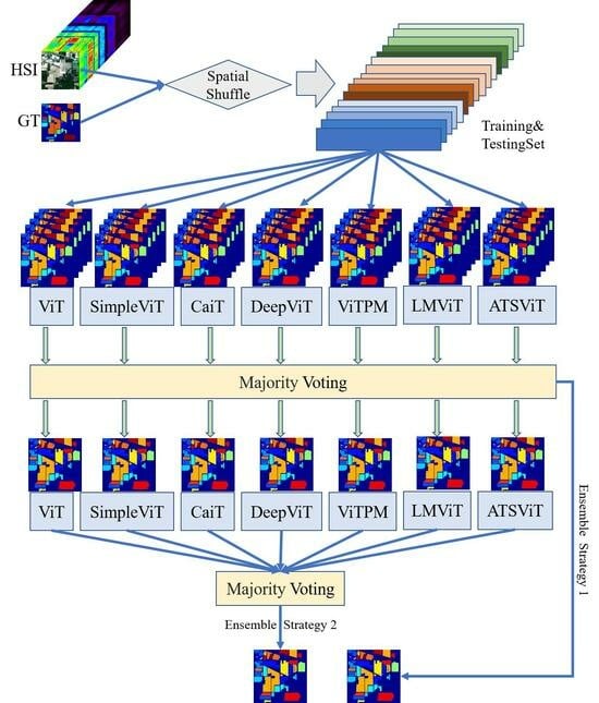
The proposed HSI classification scheme based on ensembled ViT is illustrated in Figure 1.

The ensemble strategy described in this paper consists of two levels:

At the individual model level, due to the limited number of labels in each HSI dataset, the paper only divides the dataset into training and testing sets, without creating a separate validation set. Instead, a strategy based on majority voting is used for ensemble. Specifically, after each training epoch, the trained model is used to predict the labels for all the test samples, resulting in a predicted classification map. As the training progresses, multiple predicted classification maps are generated. After several training epochs, a pixel-level majority vote is conducted on all the generated predicted classification maps. This involves counting the occurrences of each class for each pixel across the different predicted maps and selecting the class with the highest count as the final classification result for that pixel. By employing this approach, the prediction for all the test samples can be completed. This voting-based ensemble strategy takes into account the prediction results from multiple training epochs to improve classification accuracy.

At the multiple model level, two ensemble voting strategies are employed. The first strategy (Ens1) involves conducting majority voting on the predicted classification maps from all epochs of each individual method. For instance, if there are N methods and each method undergoes M epochs of training, resulting in N × M predicted classification maps, the strategy involves performing a majority vote for each pixel of the test samples among the N × M predicted results and selecting the class with the highest number of votes as the label for that pixel. The second strategy (Ens2) starts with conducting a majority vote for each individual method, resulting in predicted classification maps for the N methods. Then, another round of majority voting is performed on the predicted classification maps of each method to obtain the final predicted classification map. The distinction between these two strategies lies in the treatment of weights for each method. Since each method may have different classification performance, the number of votes obtained through majority voting may vary for each method. For example, assuming 100 epochs of training for three methods, the highest votes obtained for each test pixel might be 90, 70, and 50 for the respective methods. In the first strategy, the weights for the three methods would be calculated as follows: 90/(90 + 70 + 50) = 9/21, 70/(90 + 70 + 50) = 7/21, and 50/(90 + 70 + 50) = 5/21. However, in the second strategy, the weights for the three methods would be equal: 1/3, 1/3, and 1/3. Therefore, there could be slight differences in the final classification accuracy values of these two strategies.

3. Experiments and Results

3.1. Parameter Settings

To validate the effectiveness of the algorithm proposed in this paper, four publicly available HSI datasets were utilized, including Indian Pines (IP), Salinas Valley (SV), University of Pavia (UP), and Kennedy Space Center (KSC). Four traditional machine learning algorithms, namely multinomial logistic regression (MLR) [54], SVM [9], extreme learning machines (ELM) [55], and RF [11], were employed. Additionally, two convolutional neural network models—CNN2D [56] and PPF [57]—were utilized. Moreover, seven ViT-based algorithms, namely ViT, SimpleViT, CaiT, deepViT, ViT with Patch Merger, Learnable Memory ViT, Adaptive token sampling, and the recently proposed SpectralFormer with both pixel-wise and patch-wise models, were employed. For the seven ViT algorithms, single-level ensemble strategy and two multi-level ensemble strategies were employed to obtain classification images to facilitate a comparison in terms of algorithm performance.

The experimental system platform used in the study was Ubuntu 16.04.1 LTS, with the deep learning library being Pytorch 1.0 and Python version 3.6. The GPU hardware used was NVIDIA TITAN XP with 12 GB of VRAM.

The parameter settings for each algorithm were as follows:

-

MLR, SVM, and RF were implemented using the scikit-learn machine learning library in Python (with default parameters).

-

ELM was implemented using the scikit-elm library in Python (also with default parameters).

-

CNN2D utilized a patch size of 5 × 5. Its network structure, following the original paper’s design, consisted of two convolutional layers (3 × 3), followed by a BN (Batch Normalization) layer and ReLU activation. A fully connected layer was then employed for pixel-level classification.

-

PPF, similar to CNN2D, used a patch size of 5 × 5. The network structure was based on the original paper’s design.

The seven ViT-based algorithms share the same backbone network hyperparameters. The dimension (dim) is set to 512, the number of transformer modules (depth) is 6, the number of heads in the multi-head attention is 16, the number of neurons in the hidden layers of the multi-layer perceptron (mlp_dim) is 1024. The dropout rate for both the regular dropout and the embedding dropout is set to 0.1. The patch size is 12, and the number of input image channels (channels) is 1. The input is a 25 × B image after spatial shuffling with a 5 × 5 patch size, where B is the total number of original bands in the dataset. In the original ViT paper, a patch size of 14 or 16 is recommended. Considering that the input image of 25 × B should be evenly divided into patch size × patch size small blocks, a patch size of 12 is chosen. The input image is then resampled to 25 × 96, discarding the last row, resulting in a final input image of 24 × 96. This slightly sacrifices some input information, but since the University of Pavia dataset used in the experiment has only 103 bands while other datasets have more than 103 bands, the input image is resampled to 96 bands for the sake of using the same network architecture and maximizing the utilization of dataset. This setting can be adjusted according to the specific use case. Every one of the seven ViT variant algorithms also has specific hyperparameters. For example, in CaiT, the depth of cross-attention of CLS tokens to patch (cls_depth) is set to 2, and the layer dropout is set to 0.05. In ViT with Patch Merger, the patch_merge_layer and patch_merge_num_tokens are set to 6 and 8, respectively. In ATS, max_tokens_per_depth, which denotes the maximum number of tokens any given layer should have, is set to (256, 128, 64, 32, 16, 8). If a layer exceeds this number, it will undergo adaptive token sampling. In SpectralFormer, for the patch-wise mode, the patch size is set to 7. The results for a patch size of 5 are also provided to ensure alignment with the original paper.

3.2. IP Dataset

The IP dataset was obtained using the Airborne Visible Infrared Imaging Spectrometer (AVIRIS) sensor. It has a spectral range of 400–2500 nanometers, a spatial resolution of 20 m, and a size of 145 × 145 pixels. After excluding 24 bands with missing values or water vapor absorption, there are still 200 bands remaining. The labeled ground truth for this experiment consists of 16 land cover classes. Overall, 10% of the labeled samples were selected as training samples, while the remaining samples were used as testing samples. The specific land cover classes and sample quantities are shown in

Table 1. Land cover classes and sample quantities of IP dataset.

No	Class Name	Training Num	Testing Num
1	Alfalfa	5	41
2	Corn-notill	143	1285
3	Corn-min	83	747
4	Corn	24	213
5	Grass/Pasture	48	435
6	Grass/Trees	73	657
7	Grass/pasture-mowed	3	25
8	Hay-windrowed	48	430
9	Oats	2	18
10	Soybeans-notill	97	875
11	Soybeans-min	246	2209
12	Soybean-clean	59	534
13	Wheat	21	184
14	Woods	127	1138
15	Bldg-Grass-Tree-Drives	39	347
16	Stone-steel towers	9	84
	Total	1027	9222

.

From the classification results shown in Figure 2 (below), it can be observed that all machine learning methods—CNN2D, PPF, and SF_pixel—have a significant degree of misclassification, as indicated by the prominent noise speckles across multiple classes. Patch-based SF and ViT-based methods using the spatial shuffle strategy have achieved significant visual improvements, with a noticeable reduction in noise speckles. The ViT-based approach has even achieved close to 100% accuracy on certain classes.

Table 2. Objective evaluation of methods on IP dataset.

	MLR	SVM	RF	ELM	CNN2D	PPF	SF_Pixel	SF_Patch5	SF_Patch7
1	14.29	0.00	0.00	2.38	9.52	0.00	4.76	16.67	42.86
2	74.18	60.19	66.72	75.89	78.30	85.07	70.68	85.38	86.70
3	45.82	32.56	53.89	51.30	84.58	71.61	56.05	85.59	91.07
4	40.19	24.30	26.64	26.17	56.07	64.49	62.62	71.50	69.16
5	88.33	90.95	85.95	85.24	90.95	92.38	84.29	88.10	89.76
6	93.76	94.98	93.15	94.98	99.54	98.48	94.98	98.63	98.63
7	23.08	15.38	0.00	7.69	7.69	0.00	53.85	23.08	26.92
8	98.38	99.30	99.30	97.45	100.00	99.54	99.30	100.00	100.00
9	22.22	0.00	11.11	5.56	44.44	0.00	22.22	44.44	50.00
10	61.61	60.92	58.28	61.95	85.06	72.76	72.07	82.87	84.71
11	80.90	88.65	91.24	76.75	92.44	94.83	89.39	96.45	96.40
12	45.88	26.97	42.70	62.55	79.96	75.47	50.19	74.34	82.77
13	94.05	90.81	90.81	97.84	98.92	98.38	97.30	84.86	88.11
14	95.43	95.87	93.50	97.01	98.33	98.86	95.79	97.19	97.54
15	56.67	48.33	43.33	57.67	74.67	72.67	32.67	68.00	80.67
16	78.57	80.95	80.95	59.52	75.00	54.76	84.52	85.71	77.38
OA	75.18	72.33	75.39	75.43	87.74	86.65	78.64	88.93	90.81
AA	63.34	56.89	58.60	60.00	73.47	67.46	66.92	75.18	78.92
Kappa	71.30	67.70	71.42	71.66	85.92	84.60	75.35	87.28	89.47

and

Table 3. Objective evaluation of methods on IP dataset.

	ViT	SimpleViT	CaiT	DeepViT	ViTPM	LMViT	ATSViT	Ens1	Ens2
1	90.48	97.62	100.00	85.71	80.95	80.95	90.48	90.48	88.10
2	92.69	90.67	93.23	91.14	93.00	92.46	92.22	93.62	93.62
3	96.11	93.08	95.68	93.23	95.68	95.10	96.54	96.97	96.40
4	92.52	86.92	87.85	90.65	88.32	90.65	90.19	91.59	91.59
5	94.52	94.52	95.48	94.52	95.00	94.52	94.29	94.76	94.29
6	99.24	99.09	99.54	99.39	99.39	98.93	99.39	99.39	99.39
7	100.00	100.00	69.23	57.69	96.15	100.00	88.46	100.00	100.00
8	98.38	99.54	98.38	97.22	98.38	98.84	99.07	98.84	98.84
9	100.00	77.78	100.00	100.00	100.00	94.44	100.00	100.00	100.00
10	91.84	91.38	91.49	90.23	91.38	92.99	92.07	92.18	92.41
11	96.31	95.99	95.76	94.60	95.71	95.76	96.31	96.40	96.22
12	91.39	91.76	95.69	86.33	91.76	91.20	92.32	92.32	92.70
13	95.68	98.92	95.14	95.14	92.43	98.38	97.84	96.76	96.22
14	96.75	96.84	98.07	96.93	96.84	97.28	96.84	97.19	97.28
15	94.67	93.67	95.33	95.33	95.00	97.67	95.67	96.33	96.00
16	97.62	98.81	97.62	98.81	89.29	98.81	96.43	98.81	97.62
OA	95.19	94.53	95.41	93.70	94.79	95.18	95.26	95.67	95.57
AA	95.51	94.16	94.28	91.68	93.70	94.87	94.88	95.98	95.67
Kappa	94.51	93.76	94.76	92.82	94.06	94.50	94.59	95.05	94.94

provides the classification performance of each method on each class and the overall classification accuracy. It can be observed that the overall classification accuracy and Kappa coefficient of the machine learning methods are significantly lower compared to other methods. The PPF method even fails to correctly distinguish classes 1, 7, and 9 due to their small training sample sizes. CNN2D, SF_pixel, SF_Patch5, and SF_Patch7 also perform poorly on classes 1, 7, and 9 due to the same reason, but the Patch-based SF method performs noticeably better than the pixel-based SF method. The ViT-based method with spatial shuffle and the two ensemble strategies achieve significantly better classification accuracy compared to other methods and show clear advantages in classes with few training samples. On this dataset, the classification accuracy of the two ensemble strategies surpasses other ViT-based methods, demonstrating the stability of the ensemble strategies.

3.3. SV Dataset

The SV dataset was also acquired using the AVIRIS sensor, with an image size of 512 × 217 pixels. It includes 204 valid bands and has a spatial resolution of 3.7 m. There are 16 labeled land cover classes.

Table 4. Land cover classes and sample quantities of SV dataset.

No	Class Name	Training Num	Testing Num
1	Brocoli-gree-weeds-1	201	1808
2	Brocoli-gree-weeds-2	373	3353
3	Fallow	198	1778
4	Fallow-rough-plow	139	1255
5	Fallow-smooth	268	2410
6	Stubble	396	3563
7	Celery	358	3221
8	Grapes-untrained	1127	10,144
9	Soil-vinyard-develop	620	5583
10	Corn-senesced-green-weeds	328	2950
11	Lettuce-romaine-4wk	107	961
12	Lettuce-romaine-5wk	193	1734
13	Lettuce-romaine-6wk	92	824
14	Lettuce-romaine-7wk	107	963
15	Vinyard-untrained	727	6541
16	Vinyard-vertical-trellis	181	1626
	Total	5415	48,714

(below) displays the specific names of the 16 land cover classes, along with the quantities of the 10% training samples and 90% testing samples.

The classification results derived from using multiple methods on this dataset are shown in Figure 3 (below). It can be observed that the four machine learning methods and SF_pixel have a significant amount of misclassification in the 15th class, “Vinyard-untrained”, and they are often confused with the 8th class, “Grapes-untrained”. The main misclassification of the Patch-based SF method and the ViT-based method with spatial shuffle is that they misclassify the 8th class as the 15th class, but to a much lesser degree compared to the four machine learning methods and SF_pixel. CNN-based methods such as CNN2D and PPF perform better on these two classes compared to the machine learning methods. However, in other classes, the performance of all methods does not differ significantly, and the machine learning methods still exhibit a certain level of misclassification.

The objective evaluation results are shown in

Table 5. Objective evaluation of methods on SV dataset.

	MLR	SVM	RF	ELM	CNN2D	PPF	SF_Pixel	SF_Patch5	SF_Patch7
1	96.96	99.43	99.60	99.71	99.83	100.00	99.43	99.20	99.71
2	99.05	99.94	99.94	99.73	99.97	100.00	95.23	100.00	99.91
3	73.47	99.21	98.65	91.74	98.82	99.89	97.13	99.94	99.94
4	98.65	99.60	99.36	98.88	99.76	99.92	99.60	99.84	99.68
5	98.42	99.00	98.22	99.17	99.29	98.84	98.47	99.50	99.92
6	99.75	99.94	99.77	99.86	99.97	100.00	99.97	100.00	100.00
7	99.38	99.84	99.31	99.75	99.44	100.00	99.47	99.78	99.41
8	90.21	90.84	85.20	89.90	95.57	94.88	84.47	90.25	93.22
9	98.92	99.91	99.28	99.98	99.98	100.00	99.73	100.00	100.00
10	83.41	95.27	92.88	95.40	99.48	97.68	90.81	97.58	99.14
11	44.21	96.28	96.17	94.69	98.41	99.26	93.30	99.68	100.00
12	99.88	100.00	99.53	99.94	100.00	100.00	99.71	100.00	100.00
13	98.89	98.15	97.53	98.52	99.88	98.15	97.65	100.00	99.88
14	90.89	98.20	93.96	93.43	99.36	99.15	93.75	98.83	99.47
15	43.71	66.24	64.61	63.60	90.94	91.25	56.53	84.66	83.84
16	89.63	98.57	97.89	98.50	98.91	99.25	97.20	98.50	98.98
OA	86.44	93.02	91.16	92.06	97.63	97.48	89.45	95.64	96.28
AA	87.84	96.28	95.12	95.18	98.73	98.64	93.90	97.99	98.32
Kappa	84.81	92.20	90.15	91.14	97.36	97.20	88.23	95.14	95.85

and

Table 6. Objective evaluation of methods on SV dataset.

	ViT	SimpleViT	CaiT	DeepViT	ViTPM	LMViT	ATSViT	Ens1	Ens2
1	100.00	100.00	100.00	100.00	99.83	100.00	100.00	100.00	100.00
2	100.00	100.00	100.00	100.00	100.00	100.00	100.00	100.00	100.00
3	99.66	99.49	99.49	98.82	99.72	99.61	99.78	99.66	99.66
4	99.68	99.36	99.92	99.28	99.68	99.60	99.84	99.76	99.76
5	99.67	99.54	99.63	99.63	99.59	99.54	99.63	99.67	99.67
6	100.00	100.00	100.00	100.00	100.00	100.00	100.00	100.00	100.00
7	99.94	100.00	100.00	99.84	99.94	99.97	99.97	99.97	99.97
8	94.92	94.67	94.66	93.00	94.25	94.42	95.20	95.26	95.21
9	100.00	99.98	100.00	99.98	100.00	100.00	100.00	100.00	100.00
10	98.89	99.07	99.55	98.10	98.89	98.58	98.89	99.21	99.10
11	99.36	99.89	99.89	97.87	98.72	98.19	99.68	99.26	99.57
12	100.00	100.00	100.00	100.00	100.00	100.00	100.00	100.00	100.00
13	98.27	99.26	98.02	98.77	99.01	98.02	98.15	98.64	98.52
14	99.79	99.68	99.89	99.89	100.00	99.79	99.79	99.79	99.89
15	96.21	96.51	97.43	95.55	96.26	95.93	96.83	97.24	97.21
16	99.86	99.73	99.86	98.98	99.86	99.93	99.80	99.93	99.93
OA	98.28	98.28	98.43	97.64	98.14	98.08	98.43	98.52	98.50
AA	99.14	99.20	99.27	98.73	99.11	98.97	99.22	99.27	99.28
Kappa	98.08	98.08	98.26	97.38	97.93	97.87	98.25	98.35	98.33

. The four machine learning methods and SF_pixel have much lower accuracy on the 15th class compared to other methods. The classification accuracy of the 8th class is relatively lower compared to other classes as well, which aligns with the results of subjective visual evaluation. In terms of the OA and Kappa coefficients, the ViT-based method with spatial shuffle performs the best among all methods, followed by CNN2D and PPF. The Patch-based Spectralformer also demonstrates better performance than the pixel-based Spectralformer. Among all ViT-based methods, the accuracy of the two ensemble strategies surpasses that of individual methods, demonstrating the superiority of the ensemble strategies.

3.4. UP Dataset

The UP dataset was acquired using the Reflective Optics System Imaging Spectrometer (ROSIS) sensor and is a part of the University of Pavia campus. It has an image size of 610 × 340 pixels and consists of 103 valid bands. The spatial resolution is 1.3 m, and the spectral range spans from 430 to 860 nanometers. The ground truth of the dataset includes nine land cover classes. Overall, 10% of the labeled samples were selected as training samples. The specific land cover classes and the quantities of samples are shown in

Table 7. Land cover classes and sample quantities of UP dataset.

No	Class Name	Training Num	Testing Num
1	Asphalt	663	5968
2	Meadows	1865	16,784
3	Gravel	210	1889
4	Trees	306	2758
5	Painted metal sheets	135	1210
6	Bare Soil	503	4526
7	Bitumen	133	1197
8	Self-Blocking Bricks	368	3314
9	Shadows	95	852
	Total	4278	38,498

.

From the thematic classification map shown in Figure 4, it can be observed that the misclassified categories are mainly concentrated in Class 6 and Class 7. Similar to the SV dataset, the four machine learning algorithms and SF_pixel exhibit severe misclassification in these two classes. On the other hand, methods based on CNN and ViT perform relatively well, especially the ViT-based methods with spatial shuffle. They have lower misclassification rates compared to the SpectralFormer-based methods, demonstrating a relatively stable advantage.

The objective evaluation metrics shown in

Table 8. Objective evaluation of methods on UP dataset.

	MLR	SVM	RF	ELM	CNN2D	PPF	SF_Pixel	SF_Patch5	SF_Patch7
1	92.56	94.18	91.50	97.34	99.49	97.13	88.29	97.17	97.71
2	96.38	97.57	97.81	99.37	99.83	98.21	99.04	99.79	99.86
3	40.95	79.01	64.00	52.91	93.64	77.71	62.91	93.42	94.83
4	77.17	94.66	90.49	87.56	98.50	94.88	86.06	96.30	98.57
5	98.27	99.01	97.94	98.02	99.92	99.67	98.76	99.92	100.00
6	52.02	90.83	73.56	60.02	99.98	93.84	44.29	94.88	94.76
7	0.58	88.39	70.59	1.92	98.66	88.47	83.71	85.21	88.30
8	90.56	89.08	89.29	81.65	95.62	89.92	87.36	94.54	96.89
9	99.77	100.00	100.00	99.41	100.00	99.88	100.00	99.53	99.53
OA	82.90	94.17	90.15	86.47	98.99	95.31	86.55	97.30	97.94
AA	72.03	92.52	86.13	75.36	98.40	93.30	83.38	95.64	96.72
Kappa	76.83	92.32	86.89	81.65	98.68	93.83	81.79	96.43	97.28

and

Table 9. Objective evaluation of methods on UP dataset.

	ViT	SimpleViT	CaiT	DeepViT	ViTPM	LMViT	ATSViT	Ens1	Ens2
1	98.87	99.18	99.18	97.66	98.82	99.10	98.94	99.25	99.13
2	99.83	99.86	99.91	99.86	99.84	99.78	99.84	99.87	99.86
3	96.41	93.58	95.98	95.49	96.14	96.14	95.21	96.68	96.52
4	97.51	97.51	98.02	97.26	97.59	97.95	97.26	97.80	97.73
5	100.00	100.00	100.00	100.00	100.00	100.00	100.00	100.00	100.00
6	99.54	99.49	99.62	99.49	99.65	99.82	99.71	99.87	99.80
7	99.33	98.75	99.75	99.50	99.50	99.00	99.33	99.58	99.50
8	97.89	97.16	97.83	96.29	97.89	97.80	98.49	98.52	98.58
9	99.88	99.77	99.88	99.77	99.88	99.88	99.88	99.88	99.88
OA	99.13	98.96	99.24	98.74	99.14	99.18	99.14	99.34	99.30
AA	98.81	98.37	98.91	98.37	98.81	98.83	98.74	99.05	99.00
Kappa	98.85	98.63	99.01	98.35	98.86	98.92	98.87	99.14	99.08

also reflect the results of the subjective evaluation mentioned above. The four machine learning algorithms and SF_pixel exhibit very low accuracy on Class 6, while they perform relatively better on Class 7. On the other hand, other methods show better performance on these two classes. For example, CNN2D and the ViT-based method with spatial shuffle, as well as their ensemble strategies, achieve accuracy rates exceeding 99%. The accuracy of the two ensemble strategies is also higher than all individual ViT-based methods, indicating the effectiveness of spatial shuffle and ensemble strategies.

3.5. KSC Dataset

The KSC dataset was captured using the AVIRIS sensor at Kennedy Space Center in Florida on 23 March 1996. The dataset consists of 224 bands, with 176 bands remaining after removing water vapor noise. The images are 614 × 512 pixels in size, and the spatial resolution is 18 m. There are a total of 13 land cover classes.

Table 10. Land cover classes and sample quantities of KSC dataset.

No	Class Name	Training Num	Testing Num
1	Scrub	33	728
2	Willow swamp	23	220
3	CP hammock	24	232
4	Slash pine	24	228
5	Oak/Broadleaf	15	146
6	Hardwood	22	207
7	Swamp	9	96
8	Graminoid marsh	38	393
9	Spartina marsh	51	469
10	Cattail marsh	39	365
11	Salt marsh	41	378
12	Mud flats	49	454
13	Water	91	836
	Total	459	5752

(below) displays the specific land cover class information and sample quantities.

Figure 5 (below) presents the performance of all methods on the KSC dataset, and Figure 6 is the enlarged sub-images in the red rectangle in the ground truth image. Due to the limited number of labeled ground truth samples and the even smaller number of samples used for training, there is a significant variation in accuracy among different methods across different classes.

From the objective evaluation metrics in

Table 11. Objective evaluation of methods on KSC dataset.

	MLR	SVM	RF	ELM	CNN2D	PPF	SF_Pixel	SF_Patch5	SF_Patch7
1	96.33	96.62	95.15	97.50	99.27	98.53	93.98	98.68	100.00
2	90.87	86.76	88.58	99.09	95.89	92.24	37.44	81.28	79.00
3	71.86	61.04	83.55	85.28	94.81	84.42	0.00	84.85	87.01
4	52.86	44.93	58.59	40.09	63.00	37.89	0.00	19.38	32.60
5	35.17	40.00	55.17	44.83	66.21	35.17	0.00	0.00	3.45
6	17.39	29.47	44.93	25.12	74.40	3.38	0.00	71.01	90.82
7	23.16	75.79	89.47	20.00	96.84	0.00	0.00	92.63	100.00
8	58.59	71.35	79.95	88.02	91.93	78.91	8.07	76.04	88.02
9	88.25	95.51	96.79	87.39	100.00	89.32	76.71	80.77	81.41
10	81.59	84.62	82.97	95.33	77.20	93.96	48.90	91.21	97.25
11	97.09	95.77	95.50	93.12	99.74	98.15	93.39	100.00	97.62
12	73.95	81.46	84.99	88.52	73.73	88.74	80.57	90.07	93.60
13	99.52	100.00	99.88	99.16	94.85	99.88	100.00	100.00	100.00
OA	79.33	82.72	86.79	84.92	89.50	82.82	60.66	84.23	87.86
AA	68.20	74.10	81.19	74.11	86.76	69.27	41.47	75.84	80.83
Kappa	76.84	80.66	85.28	83.12	88.32	80.65	55.17	82.42	86.48

and

Table 12. Objective evaluation of methods on KSC dataset.

	ViT	SimpleViT	CaiT	DeepViT	ViTPM	LMViT	ATSViT	Ens1	Ens2
1	99.41	98.68	100.00	99.71	99.12	100.00	99.71	99.85	100.00
2	98.63	99.54	99.54	100.00	98.63	98.63	96.80	99.09	99.09
3	94.37	92.64	91.77	93.07	93.51	94.37	93.94	95.24	94.81
4	91.63	81.50	94.71	88.11	88.99	88.99	90.75	93.83	92.95
5	73.10	68.28	70.34	75.17	75.17	72.41	71.03	72.41	72.41
6	99.03	89.86	100.00	99.52	97.58	99.03	99.03	100.00	100.00
7	98.95	98.95	100.00	98.95	98.95	100.00	98.95	98.95	98.95
8	97.66	96.88	98.96	99.48	97.66	98.44	96.61	98.44	97.92
9	97.44	97.01	97.44	98.93	96.58	98.08	97.86	98.08	97.86
10	100.00	100.00	100.00	100.00	100.00	100.00	100.00	100.00	100.00
11	100.00	100.00	100.00	99.21	100.00	100.00	100.00	100.00	100.00
12	100.00	99.12	100.00	100.00	98.45	100.00	100.00	100.00	100.00
13	100.00	100.00	100.00	100.00	100.00	100.00	100.00	100.00	100.00
OA	97.82	96.44	98.06	98.02	97.38	97.91	97.61	98.21	98.10
AA	96.17	94.03	96.37	96.32	95.74	96.15	95.75	96.61	96.46
Kappa	97.58	96.03	97.84	97.79	97.08	97.67	97.34	98.00	97.89

(below), it can be observed that all methods exhibit low accuracy on Class 5. SF_pixel and SF_patch5 even completely misclassify this class. The ViT-based method with spatial shuffle performs relatively better. On Classes 3, 4, 6, and 7, the performances of the four machine learning methods and SF_pixel are comparatively poor, with SF_pixel being the worst. On the other hand, the ViT-based method with spatial shuffle and its ensemble strategies demonstrate good performances across all classes, with overall accuracies (OA) exceeding 96%. The OAs of the two ensemble strategies are higher than other methods, indicating that ensemble strategies can consistently achieve higher classification accuracies.

4. Discussion

4.1. Effects of Training Sample Numbers

The number of training samples is one of the key factors that impact classification accuracy. Generally, with more training samples, the final classification accuracy tends to be higher. In the previous experiments, 10% of the labeled ground truth samples were randomly selected as training samples. In this section, based on the UP dataset, 1%, 2%, and 5% of the samples were randomly chosen as training samples. The experiments were conducted using the same parameters and testing procedures as the 10% sample scenario. The OA, AA, and Kappa coefficients were calculated for different training sample proportions. The results are illustrated in Figure 7.

From the above results, it can be observed that for each specific method, increasing the sample proportion leads to a significant improvement in classification accuracy. However, the magnitude of improvement decreases as the sample proportion increases. In other words, the improvement in classification accuracy from 10% training samples compared to 5% training samples is smaller than the improvement from 5% training samples compared to 2% training samples. This implies that when the proportion reaches a certain threshold, it becomes difficult to achieve further significant improvements in classification accuracy, or in other words, it may reach 100% classification accuracy. At a specific sample proportion, the ranking of classification accuracy among all methods remains relatively consistent, and the stability of the two ensemble strategies is also verified.

4.2. Effects of Spatial Shuffle

In the previous experiments, the ViT-based method with spatial shuffle and its ensemble strategies demonstrated significant classification performances and visual advantages. To demonstrate the effect of spatial shuffle, this section selects several ViT-based methods and compares the thematic maps obtained with and without spatial shuffle on different datasets. Figure 8 (below) illustrates the comparison.

From Figure 8, it can be observed that without spatial shuffle, there are significant differences in the thematic maps, especially for classes with larger training samples, making the contrast more pronounced. This demonstrates the significant improvement in performance achieved through spatial shuffle. Figure 9 presents the classification performance of various ViT-based methods with and without spatial shuffle on four datasets. It can be seen that after incorporating spatial shuffle, all methods show a significant increase in overall accuracy, with more pronounced improvements on the IP and KSC datasets. Without spatial shuffle, the performance of the two ensemble strategies is not always superior to individual methods. However, after incorporating spatial shuffle, the ensemble strategies consistently demonstrate advantages.

5. Conclusions

The fusion of spatial–spectral information in classification methods by combining spatial and spectral features can result in higher accuracy. This has become a topic of interest in hyperspectral image classification. Generally, larger neighborhood sizes for extracting spatial features lead to higher classification accuracy, but this also introduces the problem of overlap between the training and testing sets. ViT, by segmenting the image into independent patches, achieves a classification principle different from CNN and even surpasses CNN in terms of accuracy. This is also a current research hotspot. Combining the classification results of multiple models often yields higher accuracy than individual models. In this paper, to address the issue of spatial feature extraction, a preprocessing step called spatial shuffle is introduced. By randomly shuffling the spatial pixels, it not only simulates potential patterns in the real world but also increases the training sample size. Then, an ensemble learning framework based on various variants of ViT is constructed. Through two-level ensemble strategies, high-accuracy ensembles of multiple methods are achieved. Experimental results demonstrate that incorporating spatial shuffle as a preprocessing step effectively improves the classification accuracy of individual models, and the ensemble strategies also achieve stable high accuracy. Moreover, through ensemble strategies, valuable testing samples can be fully utilized without the need for a validation set. The proposed approach consistently achieves high classification accuracy across different training sample proportions. Compared to traditional machine learning, CNN architectures, and transformer models, the proposed ensemble strategy exhibits significant advantages on multiple datasets. According to the fundamental theory of ensemble learning, the more basic the used classifiers are, the higher the possible classification accuracy. For this paper, only seven ViT-based basic classifiers were used, and the ensemble strategy was a simple average. Therefore, using more advanced ensemble strategies may also lead to higher classification accuracy, but it may also bring higher training and inference costs. However, these costs can be greatly reduced through offline training. Our future research will focus on further optimizing ViT models and constructing more powerful individual models to enhance the fine classification capability of the ensemble framework.

References

1. Ahmad, M.; Shabbir, S.; Roy, S.K.; Hong, D.; Wu, X.; Yao, J.; Khan, A.M.; Mazzara, M.; Distefano, S.; Chanussot, J. Hyperspectral Image Classification—Traditional to Deep Models: A Survey for Future Prospects. IEEE J. Sel. Top. Appl. Earth Observ. Remote Sens. 2022, 15, 968–999. [Google Scholar] [CrossRef]
2. Ramakrishnan, D.; Bharti, R. Hyperspectral Remote Sensing and Geological Applications. Curr. Sci. 2015, 108, 879–891. [Google Scholar]
3. Erives, H.; Fitzgerald, G.J. Automated Registration of Hyperspectral Images for Precision Agriculture. Proc. SPIE Int. Soc. Opt. Eng. 2005, 5544, 328–335. [Google Scholar] [CrossRef]
4. Ghiyamat, A.; Shafri, H.Z.M. A Review on Hyperspectral Remote Sensing for Homogeneous and Heterogeneous Forest Biodiversity Assessment. J. Remote Sens. 2010, 31, 1837–1856. [Google Scholar] [CrossRef]
5. Govender, M.; Chetty, K.; Bulcock, H. A Review of Hyperspectral Remote Sensing and Its Application in Vegetation and Water Resource Studies. Water SA 2009, 33, 145–151. [Google Scholar] [CrossRef]
6. Lu, G.; Fei, B. Medical Hyperspectral Imaging: A Review. J. Biomed. Opt. 2014, 19, 10901. [Google Scholar] [CrossRef]
7. Zare, A.; Bolton, J.; Chanussot, J. Foreword to the Special Issue on Hyperspectral Image and Signal Processing. IEEE J. Sel. Top. Appl. Earth Observ. Remote Sens. 2014, 7, 1841–1843. [Google Scholar] [CrossRef]
8. Ghamisi, P.; Plaza, J.; Chen, Y.; Li, J.; Plaza, A.J. Advanced Spectral Classifiers for Hyperspectral Images: A Review. IEEE Geosci. Remote Sens. Mag. 2017, 5, 8–32. [Google Scholar] [CrossRef]
9. Melgani, F.; Bruzzone, L. Classification of Hyperspectral Remote Sensing Images with Support Vector Machines. IEEE Trans. Geosci. Remote Sens. 2004, 42, 1778–1790. [Google Scholar] [CrossRef]
10. Chen, Y.; Nasrabadi, N.M.; Tran, T.D. Hyperspectral Image Classification Using Dictionary-based Sparse Representation. IEEE Trans. Geosci. Remote Sens. 2011, 49, 3973–3985. [Google Scholar] [CrossRef]
11. Ham, J.; Chen, Y.; Crawford, M.M.; Ghosh, J. Investigation of the Random Forest Framework for Classification of Hyperspectral Data. IEEE Trans. Geosci. Remote Sens. 2005, 43, 492–501. [Google Scholar] [CrossRef]
12. Bittencourt, H.R.; Oliveira Moraes, D.A.; Haertel, V. A Binary Decision Tree Classifier Implementing Logistic Regression as a Feature Selection and Classification Method and its Comparison with Maximum Likelihood. In Proceedings of the IEEE International Geoscience and Remote Symposium, Barcelona, Spain, 23–28 July 2007; pp. 1755–1758. [Google Scholar]
13. Shahshahani, B.M.; Landgrebe, D.A. The Effect of Unlabeled Samples in Reducing the Small Sample Size Problem and Mitigating the Hughes Phenomenon. IEEE Trans. Geosci. Remote Sens. 1994, 32, 1087–1095. [Google Scholar] [CrossRef]
14. Ren, J.; Zabalza, J.; Marshall, S.; Zheng, J. Effective Feature Extraction and Data Reduction in Remote Sensing Using Hyperspectral Imaging. IEEE Signal Process. Mag. 2014, 31, 149–154. [Google Scholar] [CrossRef]
15. Zabalza, J.; Ren, J.; Wang, Z.; Marshall, S.; Wang, J. Singular Spectrum Analysis for Effective Feature Extraction in Hyperspectral Imaging. IEEE Geosci. Remote Sens. Lett. 2014, 11, 1886–1890. [Google Scholar] [CrossRef]
16. Jolliffe, I.T. Principal Component Analysis. J. Mark. Res. 2002, 87, 513. [Google Scholar]
17. Li, W.; Prasad, S.; Fowler, J.E.; Bruce, L.M. Locality-Preserving Dimensionality Reduction and Classification for Hyperspectral Image Analysis. IEEE Trans. Geosci. Remote Sens. 2012, 50, 1185–1198. [Google Scholar] [CrossRef]
18. Wang, J.; Chang, C.-I. Independent Component Analysis-based Dimensionality Reduction with Applications in Hyperspectral Image Analysis. IEEE Trans. Geosci. Remote Sens. 2006, 44, 1586–1600. [Google Scholar] [CrossRef]
19. Fauvel, M.; Tarabalka, Y.; Benediktsson, J.A.; Chanussot, J.; Tilton, J.C. Advances in Spectral-Spatial Classification of Hyperspectral Images. Proc. IEEE 2013, 101, 652–675. [Google Scholar] [CrossRef]
20. Kang, X.; Xiang, X.; Li, S.; Benediktsson, J.A. PCA-based Edge-Preserving Features for Hyperspectral Image Classification. IEEE Trans. Geosci. Remote Sens. 2017, 55, 7140–7151. [Google Scholar] [CrossRef]
21. Qian, Y.; Ye, M.; Zhou, J. Hyperspectral Image Classification based on Structured Sparse Logistic Regression and Three-Dimensional Wavelet Texture Features. IEEE Trans. Geosci. Remote Sens. 2013, 51, 2276–2291. [Google Scholar] [CrossRef]
22. Cheng, G.; Li, Z.; Han, J.; Yao, X.; Guo, L. Exploring Hierarchical Convolutional Features for Hyperspectral Image Classification. IEEE Trans. Geosci. Remote Sens. 2018, 56, 6712–6722. [Google Scholar] [CrossRef]
23. Liang, M.; Jiao, L.; Yang, S.; Liu, F.; Hou, B.; Chen, H. Deep Multiscale Spectral-Spatial Feature Fusion for Hyperspectral Images Classification. IEEE J. Sel. Top. Appl. Earth Observ. Remote Sens. 2018, 11, 2911–2924. [Google Scholar] [CrossRef]
24. Wang, D.; Du, B.; Zhang, L.; Xu, Y. Adaptive Spectral-Spatial Multiscale Contextual Feature Extraction for Hyperspectral Image Classification. IEEE Trans. Geosci. Remote Sens. 2021, 59, 2461–2477. [Google Scholar] [CrossRef]
25. Wu, H.; Saurabh, P. Convolutional Recurrent Neural Networks for Hyperspectral Data Classification. Remote Sens. 2017, 9, 298–318. [Google Scholar] [CrossRef]
26. Hu, W.; Huang, Y.; Li, W.; Zhang, F.; Li, H. Deep Convolutional Neural Networks for Hyperspectral Image Classification. J. Sens. 2015, 2015, 258619. [Google Scholar] [CrossRef]
27. Wan, S.; Gong, C.; Zhong, P.; Du, B.; Zhang, L.; Yang, J. Multiscale Dynamic Graph Convolutional Network for Hyperspectral Image Classification. IEEE Trans. Geosci. Remote Sens. 2020, 58, 3162–3177. [Google Scholar] [CrossRef]
28. Dosovitskiy, A.; Beyer, L.; Kolesnikov, A.; Weissenborn, D.; Zhai, X.; Unterthiner, T.; Dehghani, M.; Minderer, M.; Heigold, G.; Gelly, S.; et al. An Image is Worth 16×16 Words: Transformers for Image Recognition at Scale. In Proceedings of the International Conference on Learning Representations (ICLR), Vienna, Austria, 4 May 2021. [Google Scholar]
29. Chen, H.; Wang, Y.; Guo, T.; Xu, C.; Deng, Y.; Liu, Z.; Ma, S.; Xu, C.; Xu, C.; Gao, W. Pre-trained image processing transformer. In Proceedings of the IEEE/CVF Conference on Computer Vision and Pattern Recognition (CVPR), Virtual Event, 19–25 June 2021; pp. 12299–12310. [Google Scholar]
30. Wang, W.; Xie, E.; Li, X.; Fan, D.-P.; Song, K.; Liang, D.; Lu, T.; Luo, P.; Shao, L. Pyramid vision transformer: A versatile backbone for dense prediction without convolutions. In Proceedings of the IEEE/CVF International Conference on Computer Vision (ICCV), Virtual Event, 10 March 2021; pp. 568–578. [Google Scholar]
31. Liu, Z.; Lin, Y.; Cao, Y.; Hu, H.; Wei, Y.; Zhang, Z.; Lin, S.; Guo, B. Swin Transformer: Hierarchical Vision Transformer Using Shifted Windows. In Proceedings of the IEEE/CVF International Conference on Computer Vision (ICCV), Virtual Event, 10 March 2021; pp. 10012–10022. [Google Scholar]
32. Wang, P.; Wang, X.; Wang, F.; Lin, M.; Chang, S.; Li, H.; Jin, R. Kvt: K-nn attention for boosting vision transformers. In Proceedings of the Computer Vision–ECCV 2022: 17th European Conference (ECCV), Tel Aviv, Israel, 23–27 October 2022; pp. 285–302. [Google Scholar]
33. Mou, L.; Zhu, X.X. Learning to pay attention on spectral domain: A spectral attention module-based convolutional network for hyperspectral image classification. IEEE Trans. Geosci. Remote Sens. 2019, 58, 110–122. [Google Scholar] [CrossRef]
34. Zhou, D.; Shi, Y.; Kang, B.; Yu, W.; Jiang, Z.; Li, Y.; Jin, X.; Hou, Q.; Feng, J. Refiner: Refining self-attention for vision transformers. arXiv 2021, arXiv:2106.03714. [Google Scholar]
35. Zhu, M.; Jiao, L.; Liu, F.; Yang, S.; Wang, J. Residual spectral–spatial attention network for hyperspectral image classification. IEEE Trans. Geosci. Remote Sens. 2020, 59, 449–462. [Google Scholar] [CrossRef]
36. He, J.; Zhao, L.; Yang, H.; Zhang, M.; Li, W. HSI-BERT: Hyperspectral image classification using the bidirectional encoder representation from transformers. IEEE Trans. Geosci. Remote Sens. 2019, 58, 165–178. [Google Scholar] [CrossRef]
37. Ali, A.; Touvron, H.; Caron, M.; Bojanowski, P.; Douze, M.; Joulin, A.; Laptev, I.; Neverova, N.; Synnaeve, G.; Verbeek, J.; et al. Xcit: Cross-covariance image transformers. In Proceedings of the Advances in Neural Information Processing Systems (NIPS), Virtual Event, 6–14 December 2021; Volume 34, pp. 20014–20027. [Google Scholar]
38. Hong, D.; Han, Z.; Yao, J.; Bojanowski, P.; Douze, M.; Joulin, A.; Laptev, I.; Neverova, N.; Synnaeve, G.; Verbeek, J.; et al. SpectralFormer: Rethinking hyperspectral image classification with transformers. IEEE Trans. Geosci. Remote Sens. 2021, 60, 1–15. [Google Scholar] [CrossRef]
39. Zhong, Z.; Li, Y.; Ma, L.; Li, J.; Zheng, W.-S. Spectral–spatial transformer network for hyperspectral image classification: A factorized architecture search framework. IEEE Trans. Geosci. Remote Sens. 2021, 60, 5514715. [Google Scholar] [CrossRef]
40. Zhang, M.; Gao, F.; Zhang, T.; Gan, Y.; Dong, J.; Yu, H. Attention Fusion of Transformer-Based and Scale-Based Method for Hyperspectral and LiDAR Joint Classification. Remote Sens. 2023, 15, 650. [Google Scholar] [CrossRef]
41. Dang, L.; Weng, L.; Hou, Y.; Liu, Y. Double-branch feature fusion transformer for hyperspectral image classification. Sci. Rep. 2023, 13, 272. [Google Scholar] [CrossRef]
42. Dang, L.; Weng, L.; Hou, Y.; Zuo, X.; Liu, Y. DSS-TRM: Deep spatial–spectral transformer for hyperspectral image classification. Eur. J. Remote Sens. 2022, 55, 103–114. [Google Scholar]
43. Li, Y.; Shi, X.; Yang, L.; Pu, C.; Tan, Q.; Yang, Z.; Huang, H. MC-GAT: Multi-layer collaborative generative adversarial transformer for cholangiocarcinoma classification from hyperspectral pathological images. Biomed. Opt. Express 2022, 13, 5794–5812. [Google Scholar] [CrossRef]
44. Zhang, T.; Wang, W.; Wang, J.; Cai, Y.; Yang, Z.; Yang, Z.; Li, J. Hyper-LGNet: Coupling Local and Global Features for Hyperspectral Image Classification. Remote Sens. 2022, 14, 5251. [Google Scholar] [CrossRef]
45. Bin, L.; Er, O.; Hu, W.; Zhang, G.; Zhao, L.; Wu, J. Multi-granularity vision transformer via semantic token for hyperspectral image classification. Int. J. Remote Sens. 2022, 43, 6538–6560. [Google Scholar]
46. Wang, W.; Liu, L.; Zhang, T.; Shen, J.; Wang, J.; Li, J. Hyper-ES2T: Efficient Spatial–Spectral Transformer for the classification of hyperspectral remote sensing images. Int. J. Appl. Earth Obs. Geoinf. 2022, 113, 103005. [Google Scholar] [CrossRef]
47. Beyer, L.; Zhai, X.; Kolesnikov, A. Better plain ViT baselines for ImageNet-1k. arXiv 2022, arXiv:2205.01580. [Google Scholar]
48. Touvron, H.; Cord, M.; Sablayrolles, A.; Synnaeve, G.; Jégou, H. Going deeper with image transformers. In Proceedings of the IEEE/CVF International Conference on Computer Vision (ICCV), Virtual Event, 10 March 2021; pp. 32–42. [Google Scholar]
49. Zhou, D.; Kang, B.; Jin, X.; Yang, L.; Lian, X.; Jiang, Z.; Hou, Q.; Feng, J. Deepvit: Towards deeper vision transformer. arXiv 2021, arXiv:2103.11886. [Google Scholar]
50. Renggli, C.; Pinto, A.S.; Houlsby, N.; Mustafa, B.; Puigcerver, J. Carlos Riquelme. Learning to merge tokens in vision transformers. arXiv 2022, arXiv:2202.12015. [Google Scholar]
51. Sandler, M.; Zhmoginov, A.; Vladymyrov, M.; Jackson, A. Fine-tuning image transformers using learnable memory. In Proceedings of the IEEE/CVF Conference on Computer Vision and Pattern Recognition (CVPR), New Orleans, LA, USA, 19 June 2022; pp. 12155–12164. [Google Scholar]
52. Fayyaz, M.; Koohpayegani, S.A.; Jafari, F.R.; Sengupta, S.; Joze, H.R.V.; Sommerlade, E.; Pirsiavash, P.H.; Gall, G. Adaptive token sampling for efficient vision transformers. In Proceedings of the European Conference on Computer Vision (ECCV), Tel Aviv, Israel, 23–27 October 2022; pp. 396–414. [Google Scholar]
53. Wang, Z.H.; Cao, B.S.; Liu, J. Hyperspectral Image Classification via Spatial Shuffle-Based Convolutional Neural Network. Remote Sens. 2023, 15, 3960. [Google Scholar] [CrossRef]
54. Haut, J.; Paoletti, M.; Paz-Gallardo, A.; Plaza, J.; Plaza, A. Cloud implementation of logistic regression for hyperspectral image classification. In Proceedings of the 17th International Conference on Computational and Mathematical Methods in Science and Engineering, CMMSE, Costa Ballena, Cádiz, Spain, 4–8 July 2017; pp. 1063–2321. [Google Scholar]
55. Li, J.; Zhao, X.; Li, Y.; Du, Q.; Xi, B.; Hu, J. Classification of hyperspectral imagery using a new fully convolutional neural network. IEEE Geosci. Remote Sens. Lett. 2018, 15, 292–296. [Google Scholar] [CrossRef]
56. Paoletti, M.E.; Haut, J.M.; Plaza, J.; Plaza, A. Deep learning classifiers for hyperspectral imaging: A review. ISPRS J. Photogramm. Remote Sens. 2019, 158, 279–317. [Google Scholar] [CrossRef]
57. Li, W.; Wu, G.; Zhang, F.; Du, Q. Hyperspectral Image Classification Using Deep Pixel-Pair Features. IEEE Trans. Geosci. Remote Sens. 2017, 55, 844–853. [Google Scholar] [CrossRef]
Figure 1. Overall flowchart of the proposed method.
Remotesensing 15 05208 g001
Figure 2. Classification results on IP dataset. (a) original HSI; (b) ground truth; (c) MLR; (d) SVM; (e) RF; (f) ELM; (g) CNN2D; (h) PPF; (i) SF_pixel; (j) SF_patch5; (k) SF_patch7; (l) ViT; (m) SimpleViT; (n) CaiT; (o) DeepViT; (p) ViTPM; (q) LMViT; (r) ATSViT; (s) Ens1; (t) Ens2.
Remotesensing 15 05208 g002aRemotesensing 15 05208 g002b
Figure 3. Classification results on SV dataset. (a) original HSI; (b) ground truth; (c) MLR; (d) SVM; (e) RF; (f) ELM; (g) CNN2D; (h) PPF; (i) SF_pixel; (j) SF_patch5; (k) SF_patch7; (l) ViT; (m) SimpleViT; (n) CaiT; (o) DeepViT; (p) ViTPM; (q) LMViT; (r) ATSViT; (s) Ens1; (t) Ens2.
Remotesensing 15 05208 g003aRemotesensing 15 05208 g003bRemotesensing 15 05208 g003c
Figure 4. Classification results on UP dataset. (a) original HSI; (b) ground truth; (c) MLR; (d) SVM; (e) RF; (f) ELM; (g) CNN2D; (h) PPF; (i) SF_pixel; (j) SF_patch5; (k) SF_patch7; (l) ViT; (m) SimpleViT; (n) CaiT; (o) DeepViT; (p) ViTPM; (q) LMViT; (r) ATSViT; (s) Ens1; (t) Ens2.
Remotesensing 15 05208 g004aRemotesensing 15 05208 g004bRemotesensing 15 05208 g004c
Figure 5. Classification results on KSC dataset. (a) original HSI; (b) ground truth; (c) MLR; (d) SVM; (e) RF; (f) ELM; (g) CNN2D; (h) PPF; (i) SF_pixel; (j) SF_patch5; (k) SF_patch7; (l) ViT; (m) SimpleViT; (n) CaiT; (o) DeepViT; (p) ViTPM; (q) LMViT; (r) ATSViT; (s) Ens1; (t) Ens2.
Remotesensing 15 05208 g005aRemotesensing 15 05208 g005b
Figure 6. Classification results on KSC dataset in the enlarged area. (a) original HSI; (b) ground truth; (c) MLR; (d) SVM; (e) RF; (f) ELM; (g) CNN2D; (h) PPF; (i) SF_pixel; (j) SF_patch5; (k) SF_patch7; (l) ViT; (m) SimpleViT; (n) CaiT; (o) DeepViT; (p) ViTPM; (q) LMViT; (r) ATSViT; (s) Ens1; (t) Ens2.
Remotesensing 15 05208 g006
Figure 7. Effects of sample numbers on UP dataset. (a) OA; (b) AA; (c) Kappa.
Remotesensing 15 05208 g007aRemotesensing 15 05208 g007b
Figure 8. Classification results with and without spatial shuffle on IP, SVm and UP datasets. (a) ViT without spatial shuffle; (b) ViT with spatial shuffle; (c) SimpleViT without spatial shuffle; (d) SimpleViT with spatial shuffle; (e) CaiT without spatial shuffle; (f) CaiT with spatial shuffle; (g) LMViT without spatial shuffle; (h) LMViT with spatial shuffle; (i) ATSViT without spatial shuffle; (j) ATSViT with spatial shuffle; (k) Ens1 without spatial shuffle; (l) Ens1 with spatial shuffle.
Remotesensing 15 05208 g008aRemotesensing 15 05208 g008b
Figure 9. Effects of spatial shuffle preprocessing on different datasets. (a) IP; (b) SV; (c) UP; (d) KSC.
Remotesensing 15 05208 g009aRemotesensing 15 05208 g009b