An Updating of the IONORT Tool to Perform a High-Frequency Ionospheric Ray Tracing

Abstract

This paper describes the main updates characterizing the new version of IONORT (IONOsperic Ray Tracing), a software tool developed at Istituto Nazionale di Geofisica e Vulcanologia to determine both the path of a high frequency (HF) radio wave propagating in the ionospheric medium, and the group time delay of the wave itself along the path. One of the main changes concerns the replacement of a regional three-dimensional electron density matrix, which was previously taken as input to represent the ionosphere, with a global one. Therefore, it is now possible to carry out different ray tracings from whatever point of the Earth’s surface, simply by selecting suitable loop cycles thanks to the new ray tracing graphical user interface (GUI). At the same time, thanks to a homing GUI, it is also possible to generate synthetic oblique ionograms for whatever radio link chosen by the user. Both ray tracing and homing GUIs will be described in detail providing at the same time some practical examples of their use for different regions. IONORT software finds practical application in the planning of HF radio links, exploiting the sky wave, through an accurate and thorough knowledge of the ionospheric medium. HF radio waves users, including broadcasting and civil aviation, would benefit from the use of the IONORT software (version 2023.10).

1. Introduction

Through the ray tracing technique, it is possible to establish the travel path of radio waves propagating in an anisotropic and inhomogeneous medium [1]. When the medium is the terrestrial ionosphere, then we talk about ionospheric ray tracing. Nevertheless, what do we really mean with the terminology ionospheric ray tracing.

Since the mid 1950s, a set of differential equations implementing Hamilton’s equations were formulated to analyze the propagation in the ionosphere of electromagnetic waves in the high frequency (HF) band (3–30 MHz) [2]. These equations cannot be solved analytically; thus, they were reformulated, and their solution was found via numerical integration techniques first by Haselgrove and Haselgrove [3] and then by Haselgrove [4]. The solutions of Haselgrove’s equations provide the paths of dominant energy flow, which are referred to as ionospheric ray tracing.

In other terms, the numerical solution of Haselgrove’s equations allows determining, once the initial point and the azimuth of the ray have been specified, the path of a HF radio wave propagating through the ionosphere from a well specified transmitting point (Tx) to an unknown landing point (Rx), being Tx and Rx any pair of points on the Earth’s surface.

The numerical approach provides a very accurate ionospheric ray tracing when a three-dimensional (3-D) electron density matrix and a geomagnetic field model are considered. In this case, we speak about a 3-D magnetoionic ray tracing. Nevertheless, the numerical ray tracing for the 3-D magnetoionic case requires very high computational costs. This is why simplified software packages, including two-dimensional (2-D) and 3-D numerical ray tracing neglecting geomagnetic field effects, and analytical ray tracings have been developed over the years.

The first codes written for the ionospheric ray tracing computation date back to the 1960s, and they provided just a numerical output with runtimes relatively long [5,6,7]. In particular, it is worth mentioning the numerical ray tracing algorithm developed by Jones [8], which was improved and modified by Jones and Stephenson [9], that became one of the best-known numerical ionospheric ray tracing codes readily available to be executed on a computer. Later on, other ray tracing algorithms were developed. Reilly [10], after a substantial revision of an earlier 3-D ionospheric ray tracing program, investigated the performance of upgraded versions of different numerical integration techniques, comparing measured oblique ionograms with synthetic ones obtained for near-vertical incidence sky wave (NVIS) conditions. In the late 1990s, the numerical Homing Ray Tracing software package developed by Norman et al. [11] was compared with the Segmented Method for 2-D Analytic Ray Tracing [12]. The latter, based on the Fully Analytic Ionospheric Model [13], outputs a reliable ray tracing through complicated horizontal gradients varying with altitude along the ray path direction. Another 2-D numerical ray tracing formulation proposed by Coleman [14] has been shown to be effective in simulating oblique and backscatter ionograms as well as the output of some ionosondes, supporting Over-The-Horizon Radar (OTHR) operations. Generally speaking, HF direction finding systems (HFDF) can provide valuable information about the angles of arrival of signals of a given frequency; this can be suitably exploited as input by a ray tracing program to determine the signal source (i.e., the transmitting site), once the electron density distribution between the HFDF site and the transmitter is known. To this regard, Huang and Reinisch [15], based on ionograms and sky-map measurements taken at a HFDF site, reconstructed in real time the 3-D electron density distribution between the HFDF site and the transmitter locations, and then used these data as input for a ray tracing program. So doing, from the measured arrival angles at the HFDF site, footprints for both the ordinary and extraordinary ray tracing in the frequency range 7–11 MHz were found to cluster around the actual position of the transmitter within an error of ≈15–55 km, depending on whether the measured ionospheric tilt is considered. More recently, Haselgrove’s equations were properly optimized and adapted for numerical integration on powerful computers, and corresponding results about ray tracing, ray homing, HF propagation-channel modeling, coordinate registration for OTHR, and the detrimental effects that travelling ionospheric disturbances (TIDs) have on an OTHR system were discussed [16]. A numerical and stepped ray tracing method, working on the empirical 3-D electron density model TWIM [17], was developed on the basis of ionospheric radio occultation data, and was successfully evaluated for oblique transmissions comparing synthetic ionograms with measured ones at Chung-Li (24.97°N, 121.19°E) [18]. The numerical 3-D ray tracing program developed by Jones and Stephenson [9] was also applied to calculate the ray paths through a polar ionosphere including patches and arcs of enhanced electron density; corresponding simulations showed satisfactory results about the ground coverage for a transmitter located at Cambridge Bay (69.1°N, 105.1°E) [19].

The Provision of High-frequency Raytracing Laboratory for Propagation studies (PHaRLAP) tool developed by Cervera and Harris [20] for studying and modelling the propagation of HF radio waves in the Earth’s ionosphere, proved to be effective in reproducing a small and a larger imposed ionospheric tilt, as well as in modeling the signatures of a TID observed on both ordinary and extraordinary traces of synthetic ionograms obtained under NVIS propagation conditions [20]. PHaRLAP was also used to model the propagation of HF signals in studies turned to the assessment of climatological models to be used for the OTHR [21], as well as to model the interference environment in the HF band, which is an important factor for both the design and the development of OTHR systems [22,23]. A modified version of the Jones and Stephenson [9] ray tracing code, taking as input different profiles of electron density derived by the International Reference Ionosphere (IRI) model ([24] and reference therein), was used to simulate the Super Dual Auroral Radar Network (SuperDARN) at African equatorial latitudes [25]. The corresponding analysis of ray tracing results obtained for an azimuth angle ranging between 1° and 360°, an elevation angle ranging between 1° and 90°, and frequencies equal to 12, 16, 20, and 24 MHz, has shown that ionospheric backscatter, as well as ground scatter, can be achieved by a SuperDARN-type radar at equatorial latitudes, in the east–west azimuthal direction [26].

When both the Tx and the Rx are known a priori, we talk about a homing approach. This method consists in sending out signals characterized by a wide range of frequencies (f), elevation angles (∆), and azimuth angle (α); the arrival point of the ray (characterized by a definite triplet: f, α, ∆) can be approximated with Rx only whether it is relatively close to the Rx position. How close the landing point is to the receiver is established evaluating whether some logical conditions have been fulfilled. However, as an alternative to the homing method, a form of variational principle could be used as the basis for calculating the ionospheric ray tracing when the landing points are known, as clearly demonstrated by Coleman [27] for several ionospheric scenarios. The homing method is, at the current time, the main approach to perform a point-to-point ionospheric ray tracing. Strangeways [28] presented a homing method capable of obtaining a precise bending of the ray paths, their phases and group delays, for both terrestrial HF links and Earth-to-satellite paths, taking into account also the effects of horizontal electron density gradients. Kashcheyev et al. [29] used a numerical homing ray tracing algorithm to estimate the impact that the second- and third-order ionospheric residuals errors have on the Global Navigation Satellite System (GNSS) positioning. They found that the greatest errors are observed when the ray paths cross the crest of the equatorial ionization anomaly. Abdullah et al. [30] considered a reference and a mobile station spaced 10 km apart to estimate the ionospheric differential error associated to ray paths of Global Positioning System (GPS) signals using the Jones and Stephenson [9] 3-D ray tracing program properly modified, and including an accurate homing procedure. They found that the differential delay is of the order of 1–5 cm at low elevation angles for both north–south and east–west directions; an amount that, even if usually neglected by the standard differential GPS method, can be important for improving the positioning results that are obtained by the single-frequency GPS users. We conclude this excursus by saying that the ionospheric ray tracing finds its main applications where a detailed knowledge of the ray path is requested; for instance, when there is a need either to predict operating frequencies or to manage HF radio communications, as well as for experimental studies on OTHR systems, single station location, and HFDF [31]. The upgrade of a whatever synoptic model with real-time ionospheric data recorded for example by a network of either ground-based ionosondes or GNSS receivers (e.g., [32,33,34,35,36,37,38] and reference therein), provides a more reliable specification of the ionospheric conditions. This is essential to enhance, through the ray tracing tool, the operation and reliability of sky-wave radio communications and radar systems beyond the line-of-sight, especially in case of Space Weather events.

At the Istituto Nazionale di Geofisica e Vulcanologia, an applicative software tool named IONORT (IONOsperic Ray Tracing) was proposed by Azzarone et al. [39] and used for more than a decade. 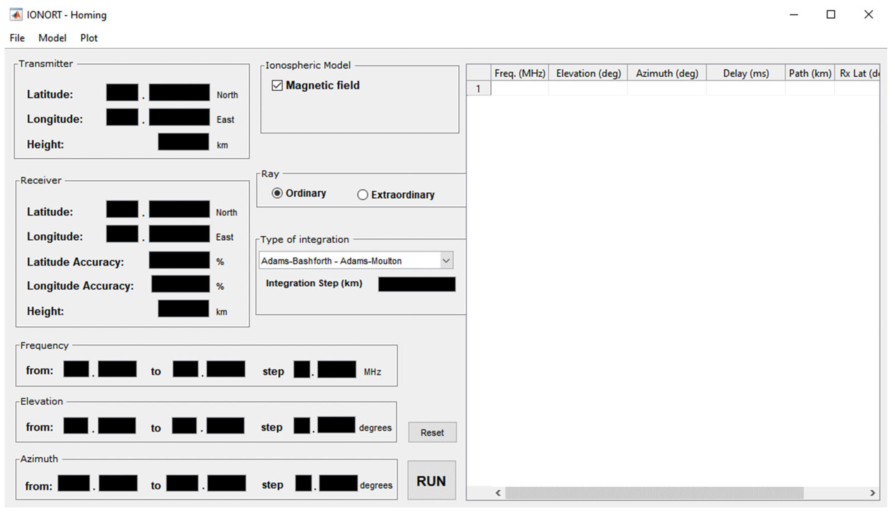Since then, the reliability of IONORT has been tested comparing synthetic and measured oblique ionograms [40,41], considering as the ionospheric background that provided by the assimilative ISP (IRI-SIRMUP-PROFILE) regional model [33,34]. In this paper, after describing the mathematical background behind IONORT, also giving a short overview of the numerical integration methods embedded in the code, we present the main upgrades recently included in IONORT. First of all, the original Fortran 77 source code was completely rewritten in Fortran 90, and carefully debugged. Secondly, the applicability of IONORT has been extended from a regional to a global scale. Finally, we present the new graphical user interfaces (GUIs) of IONORT, including a novel GUI for homing applications.

Section 2 describes the basic mathematical background of the integration computational code of IONORT. Section 3 discusses the consistency checks of the IONORT integration algorithm. Section 4 presents and discusses the main upgrades of the IONORT software package. Section 5 and Section 6 present and discuss some ray tracing and homing results. Conclusive remarks are the subject of Section 7.

2. IONORT Mathematical Background

The core of IONORT is based on the versatile computer ray tracing program developed by Jones and Stephenson [9] to trace the path of radio waves propagating in the ionosphere, that is an anisotropic, dispersive, and varying in time medium, whose index of refraction changes continuously in space. A short description of fundamental mathematical aspects on which the IONORT algorithm is based will be given. This description is, however, not exhaustive, and the most interested reader is referred to the work by Jones and Stephenson [9] for further information.

Jones and Stephenson [9] adopted the Haselgrove’s equations [3,4] for the development of their 3-D ray tracing computer program. These equations consist of a system of six coupled first-order differential equations with Hamiltonian formalism. For a geocentric spherical coordinate system (Figure 1), the first-order differential equations system assumes the following form:

$$\left\{\begin{array}{l}\frac{\mathrm{d}\rho }{\mathrm{d}P’}=-\frac{1}{c}\frac{\partial H/\partial k_{\rho }}{\partial H/\partial \omega },\\ \frac{\mathrm{d}\theta }{\mathrm{d}P’}=-\frac{1}{\rho \cdot c}\frac{\partial H/\partial k_{\theta }}{\partial H/\partial \omega },\\ \frac{\mathrm{d}\phi }{\mathrm{d}P’}=-\frac{1}{\rho \cdot c\sin \theta }\frac{\partial H/\partial k_{\phi }}{\partial H/\partial \omega },\\ \frac{\mathrm{d}{k}_{\rho }}{\mathrm{d}P’}=\frac{1}{c}\frac{\partial H/\partial \rho }{\partial H/\partial \omega }+k_{\theta }\frac{\mathrm{d}\theta }{\mathrm{d}P’}+k_{\phi }\sin \theta \frac{\mathrm{d}\phi }{\mathrm{d}P’},\\ \frac{\mathrm{d}{k}_{\theta }}{\mathrm{d}P’}=\frac{1}{\rho }\left(\frac{1}{c}\frac{\partial H/\partial \theta }{\partial H/\partial \omega }-k_{\theta }\frac{\mathrm{d}\rho }{\mathrm{d}P’}+k_{\phi }\cdot \rho \cos \theta \frac{\mathrm{d}\phi }{\mathrm{d}P’}\right),\\ \frac{\mathrm{d}{k}_{\phi }}{\mathrm{d}P’}=\frac{1}{\rho \sin \theta }\left(\frac{1}{c}\frac{\partial H/\partial \phi }{\partial H/\partial \omega }-k_{\phi }\cdot \sin \theta \frac{\mathrm{d}\rho }{\mathrm{d}P’}-k_{\phi }\cdot \rho \cos \theta \frac{\mathrm{d}\theta }{\mathrm{d}P’}\right);\end{array}\right.$$

(1)

where ρ is the distance between the origin O of the geocentric reference system and the point M (see Figure 1); θ and φ are the colatitude and the longitude in spherical polar coordinates, respectively; k_ρ, k_θ, and k_φ are the components of the wave vector k orthogonal to the wave front in the ρ, θ, and φ direction, respectively; H is the Hamiltonian, P$’$ = c·t is the group path length, being c the speed of an electromagnetic wave in the vacuum, and t the group time delay; ω = 2πf is the angular wave frequency, being f the wave frequency.

The system (1) is the one considered for calculations. Its solution allows determining the coordinates (ρ, θ, φ) reached by the wave vector, its three components (k_ρ, k_θ, k_φ), and the group time delay (t). In (1), the group path P$’$= c·t is the independent variable, because the derivatives with respect to P’ do not depend on the choice of the Hamiltonian function. This is convenient because it allows the ray tracing program taking smaller steps near the reflection point where the calculations are more critical, and a major accuracy is requested [9]. Since analytical solutions of the system (1) are not possible, numerical solutions are found by means of numerical integration techniques.

2.1. The Hamiltonian

With regard to the choice and calculation of H some issues arise. In a dissipative medium such as the ionosphere, the dispersion relation is complex, which means that H is in general complex and consequently the solutions of the system (1), i.e., the coordinates of the ray path are complex. In this case, H in the reference system of Figure 1 should be written as:

$$H=H\left(t,\rho ,\theta ,\phi ,k_{\rho },k_{\theta },k_{\phi },n^2\right)=\left\{\frac{1}{2}\left[\frac{c^2}{{\omega }^2}\left(k_{\rho }^2+k_{\theta }^2+k_{\phi }^2\right)-n^2\right]\right\},$$

(2)

where k_ρ, k_θ, k_φ, and n are complex quantities.

n² is the square of the phase refractive index for an electromagnetic wave propagating in a cold magnetized plasma with collisions, which is calculated by the following Appleton–Hartree equation:

$$n^2=1-\frac{X}{1-\mathrm{i}Z-\frac{Y_{\mathrm{T}}{}^2}{2(1-\mathrm{i}Z-X)}\pm \sqrt{\frac{Y_{\mathrm{T}}{}^4}{4{\left(1-\mathrm{i}Z-X\right)}^2}+Y_{\mathrm{L}}{}^2}},$$

(3)

being X = (f_N/f)² where f_N is the plasma frequency, Z = ν/ω where ν is the electron collision frequency, Y_T = (f_H/f)sinψ and Y_L = (f_H/f)cosψ, where f_H is the gyrofrequency and ψ the angle between the normal to the wave front and the geomagnetic field, and i = (−1)^1/2 is the imaginary unit.

Due to the birefringence of the ionospheric plasma, Equation (3) provides two refractive indices: n_ord for the ordinary ray and n_ext for the extraordinary ray, where both of them are complex quantities (being n_ord = µ_ord − iχ_ord and n_ext = µ_ext − iχ_ext) [1]. The two refractive indices are obtained from Equation (3) through the choice of either the positive or the negative sign in the denominator, which must be decided applying the so-called Booker’s rule [42]. Once the Booker’s critical frequency ω_c = (|e|B/2m_e)sin²(ψ)/cos(ψ) is defined, where B is the geomagnetic field magnitude, e is the electron charge, and m_e is the electron mass, Booker’s rule states that if ω_c/ν < 1, to achieve the continuity of µ_ord and χ_ord, in Equation (3) the positive sign must be adopted for both X < 1 and X > 1, while to achieve the continuity of µ_ext and χ_ext, in Equation (3) the negative sign must be adopted for both X < 1 and X > 1. Instead, if ω_c/ν > 1, to achieve the continuity of µ_ord and χ_ord, in Equation (3) the positive and the negative sign must be adopted, respectively, for X < 1 and for X > 1; while to achieve the continuity of µ_ext and χ_ext, in Equation (3) the negative and the positive sign must be adopted, respectively, for X < 1 and for X > 1 (e.g., [43] and reference therein).

The ray tracing in a complex space is necessary when low-frequency radio waves propagate in the ionospheric D layer, where they suffer significant energy losses. In case of HF radio waves, these losses are smaller, and their effect is only an attenuation of the signal. This is why it is desirable that the system (1) have real solutions. This is accomplished by considering H as:

$$H=H(t,\rho ,\theta ,\phi ,k_{\rho },k_{\theta },k_{\phi },n^2)=\left\{\frac{1}{2}\left[\frac{c^2}{{\omega }^2}(k^2{}_{\rho }+k^2{}_{\theta }+k^2{}_{\phi })-\mathrm{Re}(n^2)\right]\right\},$$

(4)

where the real part of the complex phase refractive index is obtained assuming ν << ω, which means that the electron collision frequency is much smaller than the wave angular frequency. In this case, in Equation (3) the term Z is negligible. Moreover, by expliciting in Equation (3) the magnetoionic parameters X, Y_T, and Y_L, i.e., writing them in terms of the plasma frequency f_N = (N_ee²/4π²ε₀m_e)^1/2 and the gyrofrequency f_H = |e|B/2πm_e, the real part of the phase refractive index assumes the following form:

$$n^2=1-\frac{\frac{N_{\mathrm{e}}(h)e^2}{4{\mathsf{\pi }}^2{\epsilon }_0{m}_{\mathrm{e}}{f}^2}}{1-\frac{{\left(\frac{\left|e\right|B}{2\mathsf{\pi }{m}_{\mathrm{e}}f}\sin \psi \right)}^2}{2\left(1-\frac{N_{\mathrm{e}}(h)e^2}{4{\mathsf{\pi }}^2{\epsilon }_0{m}_{\mathrm{e}}{f}^2}\right)}\pm \sqrt{\frac{{\left(\frac{\left|e\right|B}{2\mathsf{\pi }{m}_{\mathrm{e}}f}\sin \psi \right)}^4}{4{\left(1-\frac{N_{\mathrm{e}}(h)e^2}{4{\mathsf{\pi }}^2{\epsilon }_0{m}_{\mathrm{e}}{f}^2}\right)}^2}+{\left(\frac{\left|e\right|B}{2\mathsf{\pi }{m}_{\mathrm{e}}f}\cos \psi \right)}^2}},$$

(5)

where the signs (+) and (−) are associated to the ordinary and extraordinary propagation mode, respectively; N_e(h) is the electron density, which is function of the real height h, and ε₀ is the dielectric constant in the vacuum.

Equation (5) clearly highlights how a 3-D electron density specification of the ionosphere, as well as an Earth’s magnetic field model, are fundamental elements to obtain accurate ray tracing and homing results in the hypothesis of propagation in a collisionless ionospheric plasma.

Anyway, it must be noted that the Hamiltonian of Equation (4), which is function of the phase refractive index given by Equation (5), cannot be used when a “spitze” phenomenon occurs. This phenomenon consists of a cusp characterizing the ray path at the reflection point. It occurs when the elevation angles of the electromagnetic waves are very large, to such an extent to form a critical angle depending on the propagating wave frequency, the geomagnetic field intensity, and its inclination [44]. In this case, the phase refractive index, along with some of its derivatives, cannot be determined at the “spitze” and the Hamiltonian of Equation (4) is replaced by another Hamiltonian (see Equation (22) in [9]) which is not based on the phase refractive index.

2.2. Numerical Integration Methods Embedded in the IONORT Code

Generally, finding an analytical solution of an ordinary first-order differential equation is not always possible and, consequently, it is necessary to rely on numerical integration methods. The purpose of numerical methods is to find an approximate solution for a certain finite time interval. To solve numerically the system (1), the Runge-Kutta (R-K) method of the fourth order (R-K 4) [45] has been implemented in the IONORT source code, because it provides the best accuracy/computational cost ratio, ensuring an error for each integration step of ≈o(h⁵). Another numerical integration technique that has been implemented in the IONORT source code to solve numerically the system (1) is the Adams–Bashforth (A-B)/Adams–Moulton (A-M) predictor–corrector method, where the four-step A-B 4 method [46] is the predictor and the three-step A-M 3 method [47] is the corrector. A-B 4 and A-M 3 form a predictor–corrector pair that is a particular case of a broad category of multistep predictor–corrector methods exploiting the information from the previous steps to obtain a better approximation in the next step.

3. Consistency of the IONORT Integration Algorithm

The group time delay t is the parameter that usually a ray tracing program outputs when the numerical integration stops, and the ray has reached the ground after being reflected in the ionosphere. In principle, to test the goodness of any ray tracing algorithm, t could be compared to the group time delay as measured by OTHR applications, synchronized oblique sounding campaigns, or backscattering ionospheric soundings. Unfortunately, these kinds of measurements are uncommon. Nevertheless, taking into account the secant law, and the Breit–Tuve and Martyn propagation equivalent path theorems (e.g., [31]), an escamotage can be used. To this aim, Figure 2 shows the oblique path Tx-B_i-Rx of a HF wave propagating through the ionosphere with a frequency f_ob,i, at an elevation angle ∆, reaching the receiver after being reflected at the real height h_i, i.e., at B_i. ϕ is the incidence angle of the wave on the ionosphere that, in the approximation of a flat Earth, is simply the complementary angle of ∆. The subscript i varies from 1 to N, with N indicating different oblique frequencies reflected at different heights; consequently, also the apex of the real oblique path (B_i) and virtual triangular equivalent path (C_i) will be different, depending on how much the frequency f_ob,i penetrates the ionosphere.

The secant law states that f_ob,i = f_v,i secϕ_i, where f_v,i is the frequency that is vertically reflected at the height h_i in the middle point $B_i$ of the radio link Tx-Rx.

The Breit–Tuve theorem states that, assuming a monotonic increasing trend of the electron density profile, the group time t_i,Tx-Bi-Rx taken by the wave of frequency f_ob,i in travelling the real oblique path is equal to the time that such wave takes in travelling the virtual triangular equivalent path with speed c, that is t_i,Tx-Bi-Rx = t_i,Tx-Ci-Rx. Therefore, if N different oblique frequencies (f_ob,i with i = 1, …, N) are sent out with the same elevation angle ∆, N different real oblique paths and corresponding virtual triangular equivalent paths will be obtained so as to have t_i,Tx-Bi-Rx = t_i,Tx-Ci-Rx.

This relationship suggests that assuming as real measurements the times t_i,Tx-Ci-Rx, we can compare these to the times t_i,Tx-Bi-Rx output by IONORT, to evaluate its performance. It is clear that to do this we need to know the position of the various reflectors, which is the height of the virtual reflection points C_i. This is possible thanks to the Martyn’s theorem which establishes that, assuming valid the secant law, the virtual vertical height of reflection h’_v,i is equal to the height h’_ob,i of the virtual equivalent triangular path for the oblique signal, i.e., h’_v,i = h’_ob,i.

If a numerical electron density profile N_e = N_e (h_i) is known in the middle point of the considered radio link Tx-Rx, and neglecting the geomagnetic field in Equation (5), it is possible to calculate the group refractive index n_G as 1/n:

$$n_{\mathrm{G}}=\frac{1}{{\left(1-\frac{N_{\mathrm{e}}(h_i)e^2}{4{\mathsf{\pi }}^2{\epsilon }_{\mathrm{o}}{m}_{\mathrm{e}}{f}_{\mathrm{v},i}{}^2}\right)}^{1/2}};$$

(6)

the value of h$’$_v,i is then calculated by solving numerically the following integral:

$$h{’}_{\mathrm{v}}{}_{,i}(f_{\mathrm{v},i})=h_{\mathrm{b}}+{\displaystyle \underset{h_{\mathrm{b}}}{\overset{h_i}{\int }}{n}_{\mathrm{G}}(f_{\mathrm{v},i},N_{\mathrm{e},i}(h_i)\mathrm{d}h}={\displaystyle \underset{h_{\mathrm{b}}}{\overset{h_i}{\int }}\frac{1}{{\left(1-\frac{N_{\mathrm{e}}(h_i)e^2}{4{\mathsf{\pi }}^2{\epsilon }_{\mathrm{o}}{m}_{\mathrm{e}}{f}_{\mathrm{v},i}{}^2}\right)}^{1/2}}\mathrm{d}h},$$

(7)

where h_b and h_i are, respectively, the base of the ionosphere and the real height of reflection of the vertical path from which the wave of frequency f_v,i reflects coming back to the ground. In Equation (7), f_v,i is a parameter during the integration; therefore, the knowledge of N_e allows calculating the heights h$’$_v,i of N reflectors. Once the values of h$’$_v,i(f_v,i) are known, it is then possible to calculate t_i,Tx-Ci-Rx as follows:

$$t_{i,\mathrm{Tx}-Ci-\mathrm{Rx}}=\frac{2\sin \left(\frac{D}{2R_{\mathrm{T}}}\right)\cdot \left[R_{\mathrm{T}}+h{’}_{\mathrm{v},i}\right]}{c\cdot \cos (\Delta )},$$

(8)

where D, R_T and ∆ are known.

Specifically, in order to fully test the IONORT algorithm, a numerical 3-D electron density background was considered, and three runs have been carried out, for three different values of ∆: 18°, 30°, and 45°. For each run, IONORT takes as input parameters values of f_ob,i ranging between 3 and 30 MHz. In this way, three different datasets of IONORT times are obtained. Subsequently, each dataset was compared with the corresponding one calculated through Equation (8). According to the Breit–Tuve theorem, datasets corresponding to the same elevation angle should be equal. As a consequence, the following comparison t_i,Tx-Bi-Rx vs. t_i,Tx-Ci-Rx has been carried out for each of the three chosen elevation angles.

An example of this analysis is shown in Figure 3 for ∆ = 30°, where the percentage relative error:

$$\Delta t_i=\frac{\left|t_{i,\mathrm{Tx}-B_i-\mathrm{Rx}}-t_{i,\mathrm{Tx}-C_i-\mathrm{Rx}}\right|}{t_{i,\mathrm{Tx}-C_i-\mathrm{Rx}}}\cdot 100$$

(9)

is also reported.

The trend of Δt_i given by Equation (9) represents the performance of the IONORT algorithm, and shows that for low frequencies, from 3 to about 12 MHz, the percentage relative error is below 1%. Smaller errors at lower frequencies are those related to waves travelling for relatively short paths; in this case, the Earth’s curvature can be neglected and the approximation of flat ionospheric layers is more appropriate, leading to a reduction in the error that can be ascribed only to the integration procedure used by IONORT. The errors increase when getting closer to the maximum of electron density and then decrease again showing a fluctuating trend that practically does not ever exceed 3%.

The outcome of Figure 3 holds also for elevation angles equal to 18° and 45°, for which the results are not shown here. The interested reader can refer to the work by Bianchi et al. [48] where additional details about this issue can be found.

4. Main IONORT Upgrades

Compared to Azzarone et al. [39], the IONORT tool was upgraded from both the source code point of view and the graphical design point of view.

Concerning the code, this was completely rewritten from Fortran 77 to Fortran 90 programming language, several bugs have been fixed and, at the same time, some pointless parts of the code have been removed and the existing routines have been optimized. As a result, an improvement of the running speed was obtained.

The conversion from Fortran 77 to Fortran 90 programming language has allowed to solve the significant problem affecting the previous version that forced the user to work with a regional electron density background, limited in both latitude and longitude. Now the user can work with a global electron density background, for instance that given by the IRI model [24], and generate both numerical ray tracing data, for whatever transmitting point on the Earth’s surface, and numerical homing data for any Tx-Rx pair in the world.

The Matlab programming language has been employed for developing a new graphical design. In fact, there are many updates regarding the GUI. The first one concerns the possibility, when launching IONORT, to choose what procedure to launch: ray tracing or homing (Figure 4).

4.1. The Ray Tracing GUI

A new version of the ray tracing GUI was developed (Figure 5), that gives the user the possibility to select nested loop cycles and visualize the ray tracing results, whatever is the transmitting point chosen on the Earth’s surface. On the left side, the user has the possibility to insert the coordinates of the transmitting point and the desired loop cycles in frequency, elevation, and azimuth angles, as well as to choose the integration algorithm. In the central part, the user can include the geomagnetic field and choose both the kind of ray (ordinary or extraordinary) and the integration step. The results of the ray tracing are shown both in the lower part of the GUI as an altitude vs. ground range plot, and in the right side of the GUI as rays on the Earth’s surface.

4.2. The Homing GUI

Another novelty is the inclusion of a homing GUI (Figure 6), which allows visualizing a synthetic oblique ionogram for whatever radio link the user wants to simulate on the terrestrial surface. As for the ray tracing GUI, the user can insert the loop cycles in frequency, elevation angle, and azimuth angles, and choose the kind of ray to be processed (ordinary or extraordinary), the type of integration and the corresponding step, and whether the run has to be carried out with or without the geomagnetic field. The right side of the GUI shows the list of the “winner triplets”, while the frequencies and group time delays values are automatically plotted to visualize the corresponding synthetic oblique ionogram. The winner triplets are the values of frequency, elevation, and azimuth angle, embedded in the loop cycles, thanks to which the electromagnetic wave sent out from the Tx reaches the Rx, on the basis of the chosen accuracy values. On the left side, the user, besides inserting the coordinates of both the transmitting and receiving points, can also insert the accuracy values requested along the directions north–south and east–west. It is worth saying a few words about the meaning of parameters Latitude Accuracy and Longitude Accuracy, which are chosen for running the homing procedure, because they are fundamental for the verification of the homing. The values Latitude Accuracy and Longitude Accuracy are those for which it is requested that the following logical conditions are fulfilled:

$$\begin{gathered} \left[\frac{{\lambda }_{\mathrm{Rx}}-{\lambda }_{\mathrm{LandingPoint}}}{(\mathsf{\pi }/2)-{\lambda }_{\mathrm{Rx}}}\right]\cdot 100\le \mathit{Latitude\; Accuracy} \\ \mathrm{AND} \\ \left[\frac{{\phi }_{\mathrm{LandingPoint}}-{\phi }_{\mathrm{Rx}}}{{\phi }_{\mathrm{Rx}}}\right]\cdot 100\le \mathit{Longitude\; Accuracy} \end{gathered}$$

(10)

where λ_Rx and φ_Rx are the latitude and longitude of the receiver, while λ_LandingPoint and φ_LandingPoint are the latitude and longitude of the landing point. Whenever the condition (10) is fulfilled, the homing subroutine assumes that the position of the landing point can be approximated with the position of the receiver. In this case, the homing is considered successful. When this circumstance is verified for a given “triplet” (f, α, ∆), then a point, whose coordinates are the frequency and the time delay, is drawn so as to obtain at the end of the nested loop cycle a synthetic oblique ionogram, as shown in Section 6.

It is worth highlighting that the input settings to be inserted in both GUIs can be saved as a Matlab file. This is a very useful feature whenever the user wants to repeat the same ray tracing or homing analysis, because this file can be loaded by opening the menu “File” and clicking “Load Input data”, thus avoiding rewriting each time the same settings.

5. The Ray Tracing Feature: Some Results

In this section, two ray tracing cases obtained by placing the transmitter at high and middle latitude in the Northern hemisphere will be shown. The electron density background will be that provided by the IRI model [24], based on both the 12-month smoothed ionospheric index (IG₁₂) [49] and the 12-month smoothed sunspot number index (R₁₂) [50,51]. The ray tracing simulations have been performed using as integration method that of A-B/A-M, setting the ordinary (O) mode of propagation, and considering as geomagnetic field model the International Geomagnetic Reference Field (IGRF-13) [52]. To highlight the global potentialities of IONORT, additional examples can be found in the Supplementary Material.

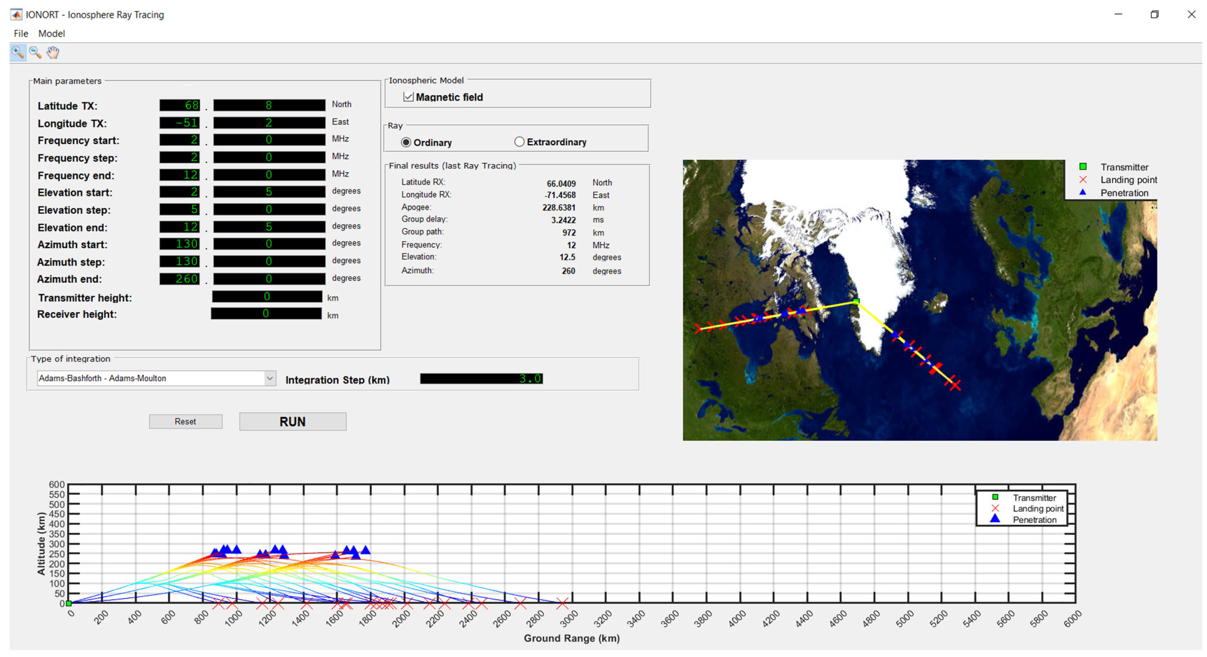
Figure 7 shows the ray tracing results for the O propagation mode for the epoch 6 January 2022 at 09:00 UT, simulating a transmitter positioned at Qasigiannguit (68.8°N, 51.2°W, Greenland), and setting loop cycles in frequency from 2 to 12 MHz (with a step of 2 MHz), and in elevation angle from 2.5° to 12.5° (with a step of 5°). Two values of the azimuth angle equal to 130° and 260° have been considered. For α = 130° the minimum length path (≈992 km, group delay ≈ 3.3112 ms) occurs for f = 2 MHz and ∆ = 7.5°, while the maximum length path (≈2448 km, group delay ≈ 8.1672 ms) occurs for f = 8 MHz and ∆ = 2.5°. For α = 260° the minimum length path (≈917 km, group delay ≈ 3.0685 ms) occurs for f = 2 MHz and ∆ = 12.5°, while the maximum length path (≈3013 km, group delay ≈ 10.0525 ms) occurs for f = 8 MHz and ∆ = 2.5°.

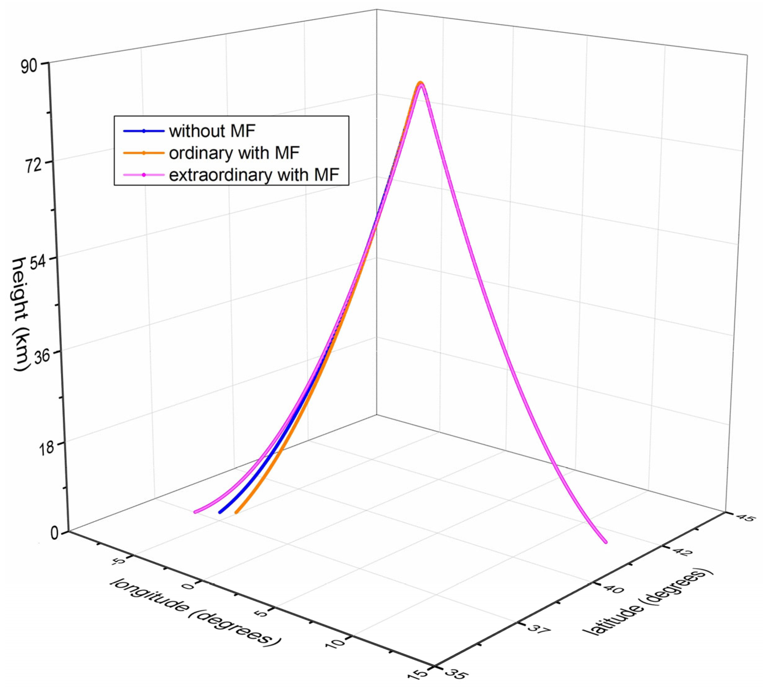
The same settings used to obtain the results shown in Figure 7 for the O propagation mode, were used to run IONORT for both the extraordinary (X) propagation mode and without including the geomagnetic field. The corresponding results are not shown here. Nevertheless, an example of the obtained ray paths for the O and X modes, as well as in absence of the geomagnetic field, are shown in Figure 8 for f = 6 MHz, ∆ = 12.5° and α = 130°.

In addition, the azimuthal displacement due to the anisotropy introduced by the presence of the Earth’s magnetic field has been calculated also for some of ray tracings drawn in the 2-D plot shown in Figure 7. Corresponding results are shown in

Table 1. Azimuthal displacement showed by the O propagation mode due to the presence of the geomagnetic field, for some of ray tracings of Figure 7, whose frequency and elevation angle are written in the first column.

f (MHz), ∆ (°)	αstart = 130° ∆α° (O)	αstart = 260° ∆α° (O)
4, 2.5	0.059	0.123
4, 12.5	0.280	0.211
6, 2.5	0.099	0.085
6, 7.5	0.161	0.132
6, 12.5	0.396	0.226
8, 2.5	0.090	0.085

, where α_start is the initial azimuth angle given as input through the GUI.

Figure 9 shows the ray tracing results for the O propagation mode for the epoch 24 May 2022 at 15:00 UT simulating a transmitter positioned in Rome (41.9°N, 12.5°E; Italy), with the same loop cycles of Figure 7. Azimuth angles equal to 110° and 260° have been chosen. For α = 110° the minimum length path (≈729 km, group delay ≈ 2.4319 ms) occurs for f = 2 MHz and ∆ = 12.5°, while the maximum length path (≈2054 km, group delay ≈ 6.8546 ms) occurs for f = 12 MHz and ∆ = 12.5°. For α = 260° the minimum length path (≈728 km, group delay ≈ 2.4293 ms) occurs for f = 2 MHz and ∆ = 12.5°, while the maximum length path (≈1768 km, group delay ≈ 5.9003 ms) occurs for f = 12 MHz and ∆ = 2.5°.

As carried out for the previous epoch, also in this case the same settings used to obtain the results shown in Figure 9 for the O mode of propagation, were used to run IONORT for both the X propagation mode and without including the geomagnetic field. An example of the obtained ray paths calculated for the O and X modes, as well as in absence of the geomagnetic field, are shown in Figure 10 for f = 2 MHz, ∆ = 2.5 °, and α = 260°.

In addition, the azimuthal displacement due to the anysotropy introduced by the presence of the Earth’s magnetic field has been calculated also for some of ray tracings drawn in the 2-D plot shown in Figure 9. Corresponding results are shown in

Table 2. Azimuthal displacement showed by the O propagation mode due to the presence of the geomagnetic field, for some of ray tracings of Figure 9, whose frequency and elevation angle are written in the first column.

f (MHz), ∆ (°)	αstart = 110° ∆α° (O)	αstart = 260° ∆α° (O)
4, 2.5	0.071	0.038
4, 12.5	0.075	0.040
6, 2.5	0.070	0.038
6, 7.5	0.072	0.039
6, 12.5	0.075	0.039
8, 2.5	0.070	0.038

, where α_start is the initial azimuth angle given as input through the GUI.

Comparing Table 1 with Table 2 it is clear how the effect of the geomagnetic field is more important at high latitudes than at middle latitudes. A larger value of the geomagnetic field at high latitudes causes a larger azimuthal displacement of the plane of propagation than at middle latitudes.

6. The Homing Feature: Some Results

In this section, two homing cases obtained by placing the transmitter and the receiver both in the Northern Europe and Middle East will be shown. As it was carried out in the previous section, the electron density background will be that output by the IRI model [24]. The homing simulations will be performed using as integration method the A-B/A-M, setting both modes of propagation, O and X, and considering as geomagnetic field model the International Geomagnetic Reference Field (IGRF-13) [52]. Moreover, different loop cycles in frequency, elevation angle, and azimuth angle are tried to find the “winner triplets”, namely those combinations of (f, ∆, α) that allow the homing. The synthetic oblique ionograms resulting from the homing will be shown superimposed to the list of the “winner triplets”. To highlight the global potentialities of IONORT, additional examples can be found in the Supplementary Material.

Figure 11 shows the homing result obtained for the epoch 9 August 2022 at 23:00 UT, for the O mode, simulating a transmitter located in London (51.5°N, 359.8°E; England) and a receiver located in Stockholm (59.3°N, 18.0°E; Sweden). The corresponding oblique ionogram shows a Maximum Usable Frequency (MUF) for the simulated radio link (ground range ≈ 1433 km) of 8.7 MHz.

Figure 12 shows the homing result for the same radio link considered in Figure 11, for the X propagation mode. The corresponding oblique ionogram shows that the MUF is now 9.3 MHz.

In Figure 13 the O and X trace have been plotted together to better visualize their differences.

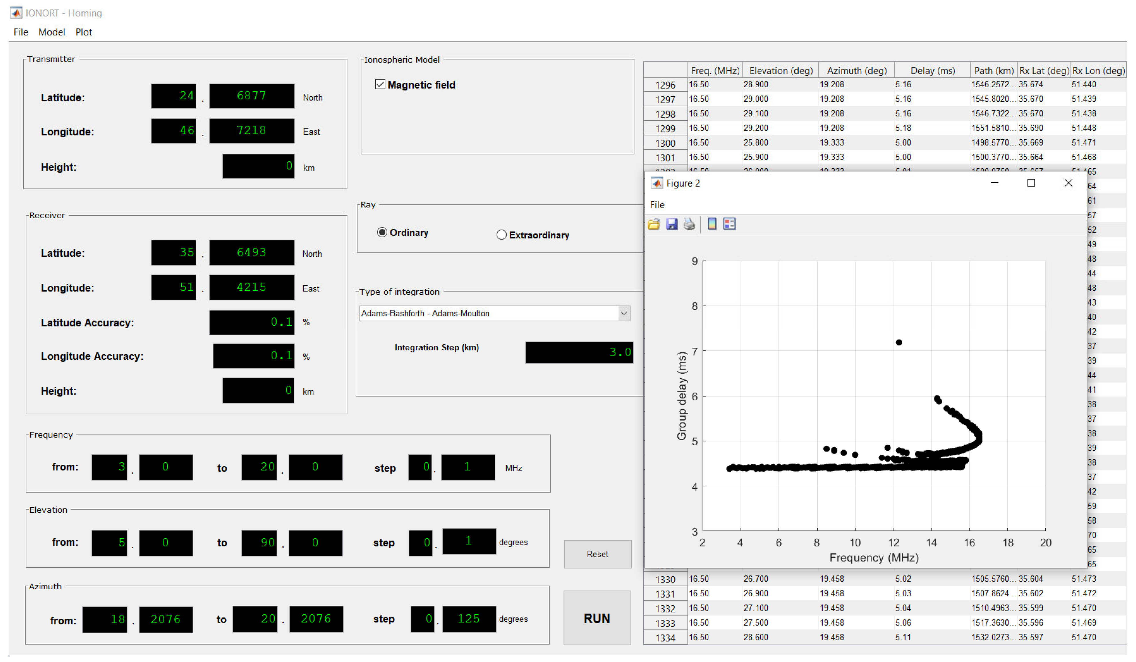
Figure 14 shows the homing result obtained for the epoch 29 July 2022 at 09:00 UT, for the O mode, simulating a transmitter located in Ryadh (24.6°N, 46.7°E; Saudi Arabia) and a receiver located at Teheran (35.6°N, 51.4°E; Iran). The oblique ionogram corresponding to the simulated radio link (ground range ≈ 1294 km) is constituted by two well distinct traces: the lower trace is related to the F1-layer, characterized by a MUF of about 16.0 MHz; the upper trace is related to the F2-layer, characterized by a MUF of 16.5 MHz.

Figure 15 shows the homing result for the same radio link considered in Figure 14, for the X propagation mode. The corresponding oblique ionogram shows a lower trace related to the F1-layer, characterized by a MUF slightly larger than 16.0 MHz, and an upper trace, related to the F2-layer, showing a MUF of 16.8 MHz.

As it was carried out for the previous case, in Figure 16 the O and X trace have been plotted together to better visualize their differences.

Comparing Figure 13 with Figure 16 it is clear how a larger value of the geomagnetic field at higher latitudes causes a larger difference between the O and X MUF values.

7. Conclusive Remarks

In this paper, the main novelties characterizing the new version of IONORT (version 2023.10), with respect to the previous one proposed by Azzarone et al. [39], have been shown and discussed. In particular, the most important improvement is that now the users can perform their own simulations anywhere in the world. Moreover, besides a ray tracing simulation, now a user has also the possibility to perform a homing simulation, obtaining as output all the triplets (frequency, elevation angle, and azimuth angle) that satisfy the initial conditions chosen in terms of accuracy values requested along the directions north–south and east–west. It is worth highlighting that all the simulations described in the paper have been performed using as electron density background that given by the IRI model [24]. Moreover, a user can use any other ionospheric model; obviously, the important thing is to respect the electron density matrix format currently in force. In this regard, one thing that needs to be underlined is that the IRI model is a climatological model, and consequently its use in the Space Weather context could be limiting [53]. With regard to this, the consideration of nowcasting methods, as for instance the IRI UPdate [35] or the IRI Real Time Assimilative Model [32], could be more appropriate. With regard to future developments, it is currently under study the calculation of the nondeviative absorption due to the propagation through the D layer. A further possible work could be based on testing IONORT under severe Space Weather events and comparing the results obtained with both a climatological and a nowcasting background.

References

1. Budden, K.G. The Propagation of Radio Waves: The Theory of Radio Waves of Low Power in the Ionosphere and Magnetosphere; Cambridge University Press: Cambridge, UK, 1988; p. 688. [Google Scholar]
2. Haselgrove, J. Ray Theory and a New Method for Ray Tracing. In The Physics of the Ionosphere: Report of the Physical Society Conference, Held at Cavendish Laboratory, Cambridge, September 1954; Physical Society: London, UK, 1955; pp. 355–364. [Google Scholar]
3. Haselgrove, C.B.; Haselgrove, J. Twisted ray paths in the ionosphere. Proc. Phys. Soc. 1960, 75, 357–363. [Google Scholar] [CrossRef]
4. Haselgrove, J. The Hamilton ray path equations. J. Atmos. Terr. Phys. 1963, 25, 397–399. [Google Scholar] [CrossRef]
5. Dudziak, W.F. Three-Dimensional Ray Trace Computer Program for Electromagnetic Wave Propagation Studies; Technical Military Planning Operation RM 61TMP-32, Defense Atomic Support Agency DASA 1232; General Electrical Company: Santa Barbara, CA, USA, 1961; p. 170. [Google Scholar]
6. Lawrence, R.S.; Posakony, D.J. A digital ray tracing program for ionospheric research. In Proceedings of the Second International Space Science Symposium, Florence, Italy, 10–14 April 1961; van de Hulst, H.C., de Jager, C., Moore, A.F., Eds.; North-Holland Publishing Co.: Amsterdam, The Netherlands; New York, NY, USA, 1961; Volume 2, pp. 258–276. [Google Scholar]
7. Croft, T.A.; Gregory, L. Fast, Versatile Ray-Tracing Program for IBM 7090 Digital Computers; Defense Technical Information Center, Ed.; Rept. SEL-63-107, TR 82, Contract No. 225 (64); Office of Naval Research, Advanced Research Projects Agency: Stanford, CA, USA, 1963; p. 28.
8. Jones, R.M. A Three Dimensional Ray Tracing Computer Program; ESSA Technical Report, IER 17-ITSA 17; Government Printing Office: Washington, DC, USA, 1966.
9. Jones, R.M.; Stephenson, J.J. A Versatile Three-Dimensional Ray Tracing Computer Program for Radiowaves in the Ionosphere; OT Report, 75–76; U.S. Department of Commerce, Office of Telecommunication, U.S. Government Printing Office: Washington, DC, USA, 1975.
10. Reilly, M.H. Upgrades for efficient three-dimensional ionospheric ray-tracing: Investigation of HF near vertical incidence sky wave effects. Radio Sci. 1991, 26, 971–980. [Google Scholar] [CrossRef]
11. Norman, R.J.; Bennett, J.A.; Dyson, P.L.; Nguyen, L. HIRT: Homing-in Ray Tracing Program; Research report; School of Physics, La Trobe University: Bundoora, VIC, Australia, 1994. [Google Scholar]
12. Norman, R.J.; Cannon, P.S. A two-dimensional analytic ray tracing technique accommodating horizontal gradients. Radio Sci. 1997, 32, 387–396. [Google Scholar] [CrossRef]
13. Anderson, D.N.; Forbes, J.M.; Codrescu, M. A fully analytic, low- and middle-latitude ionospheric model. J. Geophys. Res. 1989, 9, 1520–1524. [Google Scholar] [CrossRef]
14. Coleman, C.J. A ray-tracing formulation and its application to some problems in over-the-horizon radar. Radio Sci. 1998, 33, 1187–1197. [Google Scholar] [CrossRef]
15. Huang, X.; Reinisch, B. Real Time HF ray tracing through a tilted ionosphere. Radio Sci. 2006, 41, RS5S47. [Google Scholar] [CrossRef]
16. Nickisch, L.J. Practical applications of Haselgrove’s equations for HF systems. Radio Sci. Bull. 2008, 325, 36–48. [Google Scholar]
17. Tsai, L.C.; Liu, C.H.; Hsiao, T.Y.; Huang, J.Y. A near real-time phenomenological model of ionospheric electron density based on GPS radio occultation data. Radio Sci. 2009, 44, RS5002. [Google Scholar] [CrossRef]
18. Tsai, L.C.; Liu, C.H.; Huang, J.Y. Three-dimensional numerical ray tracing on a phenomenological ionospheric model. Radio Sci. 2010, 44, RS5017. [Google Scholar] [CrossRef]
19. Warrington, E.M.; Zaalov, N.Y.; Naylor, J.S.; Stocker, A.J. HF propagation modeling within the polar ionosphere. Radio Sci. 2012, 47, RS0L13. [Google Scholar] [CrossRef]
20. Cervera, M.A.; Harris, T.J. Modeling ionospheric disturbance features in quasi-vertically incident ionograms using 3-D magnetoionic ray tracing and atmospheric gravity waves. J. Geophys. Res. Space Phys. 2014, 119, 431–440. [Google Scholar] [CrossRef]
21. Cervera, M.A.; Francis, D.B.; Frazer, G.J. Climatological Model of Over-the-Horizon Radar. Radio Sci. 2018, 53, 988–1001. [Google Scholar] [CrossRef]
22. Pederick, L.K.; Cervera, M.A. Modeling the interference environment in the HF band. Radio Sci. 2016, 51, 82–90. [Google Scholar] [CrossRef]
23. Pederick, L.K.; Cervera, M.A. A directional HF noise model: Calibration and validation in the Australian region. Radio Sci. 2016, 51, 25–39. [Google Scholar] [CrossRef]
24. Bilitza, D.; Pezzopane, M.; Truhlik, V.; Altadill, D.; Reinisch, B.W.; Pignalberi, A. The International Reference Ionosphere model: A review and description of an ionospheric benchmark. Rev. Geophys. 2022, 60, e2022RG000792. [Google Scholar] [CrossRef]
25. Greenwald, R.A.; Baker, K.B.; Dudeney, J.R.; Pinnock, M.; Jones, T.B.; Thomas, E.C.; Villain, J.-P.; Cerisier, J.-C.; Senior, C.; Hanuise, C.; et al. DARN/SuperDARN: A global view of the dynamics of high-latitude convection. Space Sci. Rev. 1995, 71, 761–796. [Google Scholar] [CrossRef]
26. Michael, C.M.; Yeoman, T.K.; Wright, D.M.; Milan, S.E.; James, M.K. A Ray Tracing Simulation of HF Ionospheric Radar Performance at African Equatorial Latitudes. Radio Sci. 2020, 55, e2019RS006936. [Google Scholar] [CrossRef]
27. Coleman, C.J. Point-to-point ionospheric ray tracing by a direct variational method. Radio Sci. 2011, 46, RS5016. [Google Scholar] [CrossRef]
28. Strangeways, H.J. Effects of horizontal gradients on ionospherically reflected or transionospheric paths using a precise homing-in method. J. Atmos. Sol. Terr. Phys. 2000, 62, 1361–1376. [Google Scholar] [CrossRef]
29. Kashcheyev, A.; Nava, B.; Radicella, S.M. Estimation of higher-order ionospheric errors in GNSS positioning using a realistic 3-D electron density model. Radio Sci. 2012, 47, RS4008. [Google Scholar] [CrossRef]
30. Abdullah, M.; Strangeways, H.J.; Zulkifli, S.S.N. Ionospheric differential error determination using ray tracing for a short baseline. Adv. Space Res. 2010, 46, 1326–1333. [Google Scholar] [CrossRef]
31. McNamara, L.F. The Ionosphere: Communications, Surveillance, and Direction Finding; Krieger Pub Co., Technical Book Store: Malabar, FL, USA, 1991; p. 248. [Google Scholar]
32. Galkin, I.A.; Reinisch, B.W.; Huang, X.; Bilitza, D. Assimilation of GIRO data into a real-time IRI. Radio Sci. 2012, 47, RS0L07. [Google Scholar] [CrossRef]
33. Pezzopane, M.; Pietrella, M.; Pignatelli, A.; Zolesi, B.; Cander, L.R. Assimilation of autoscaled data and regional and local ionospheric models as input sources for real-time 3-D International Reference Ionosphere modeling. Radio Sci. 2011, 46, RS5009. [Google Scholar] [CrossRef]
34. Pezzopane, M.; Pietrella, M.; Pignatelli, A.; Zolesi, B.; Cander, L.R. Testing the three-dimensional IRI-SIRMUP-P mapping of the ionosphere for disturbed periods. Adv. Space Res. 2013, 52, 1726–1736. [Google Scholar] [CrossRef]
35. Pignalberi, A.; Pezzopane, M.; Rizzi, R.; Galkin, I. Effective solar indices for ionospheric modeling: A review and a proposal for a real-time regional IRI. Surv. Geophys. 2018, 39, 125–167. [Google Scholar] [CrossRef]
36. Pignalberi, A.; Pietrella, M.; Pezzopane, M.; Rizzi, R. Improvements and validation of the IRI UP method under moderate, strong, and severe geomagnetic storms. Earth Planets Space 2018, 70, 180. [Google Scholar] [CrossRef]
37. Pignalberi, A.; Habarulema, J.B.; Pezzopane, M.; Rizzi, R. On the development of a method for updating an empirical climatological ionospheric model by means of assimilated vTEC measurements from a GNSS receiver network. Space Weather 2019, 17, 1131–1164. [Google Scholar] [CrossRef]
38. Pietrella, M.; Pezzopane, M.; Zolesi, B.; Cander, L.R.; Pignalberi, A. The Simplified Ionospheric Regional Model (SIRM) for HF Prediction: Basic Theory, Its Evolution and Applications. Surv. Geophys. 2020, 41, 1143–1178. [Google Scholar] [CrossRef]
39. Azzarone, A.; Bianchi, C.; Pezzopane, M.; Pietrella, M.; Scotto, C.; Settimi, A. IONORT: A Windows soft-ware tool to calculate the HF ray tracing in the ionosphere. Comput. Geosci. 2012, 42, 57–63. [Google Scholar] [CrossRef]
40. Settimi, A.; Pezzopane, M.; Pietrella, M.; Bianchi, C.; Scotto, C.; Zuccheretti, E.; Makris, J. Testing the IONORT-ISP system: A comparison between synthesized and measured oblique ionograms. Radio Sci. 2013, 48, 167–179. [Google Scholar] [CrossRef]
41. Pietrella, M.; Pezzopane, M.; Settimi, A. Ionospheric response under the influence of the solar eclipse occurred on 20 March 2015: Importance of autoscaled data and their assimilation for obtaining a reliable modeling of the ionosphere. J. Atmos. Sol. Terr. Phys. 2016, 146, 49–57. [Google Scholar] [CrossRef]
42. Booker, H.G. The application of the magnetoionic theory to the ionosphere. Proc. R. Soc. Lond. Ser. A Math. Phys. Sci. 1935, 150, 267–286. [Google Scholar] [CrossRef]
43. Settimi, A. An in-depth analysis on the Quasi-Longitudinal approximations applied to ionospheric ray-tracing, oblique and vertical sounding, and absorption. Ann. Geophys. Italy 2022, 65, PA003. [Google Scholar] [CrossRef]
44. Elias, A.G.; Fagre, M.; Zossi, B.S.; Amite, H. Spitze Angle Changes during Rapid Geomagnetic Core Field Variation. Geomagn. Aeron. 2021, 61, 134–142. [Google Scholar] [CrossRef]
45. Bachvalov, N.S. Metodi Numerici; Editori Riuniti University Press: Rome, Italy, 2012; p. 620. (In Italian) [Google Scholar]
46. Butcher, J.C. Numerical Methods for Ordinary Differential Equations; John Wiley: Hoboken, NJ, USA, 2003; p. 103. [Google Scholar] [CrossRef]
47. Hairer, E.; Nørsett, S.P.; Wanner, G. Solving Ordinary Differential Equations I: Nonstiff Problems, 2nd ed.; Springer: Berlin, Germany, 1993. [Google Scholar]
48. Bianchi, C.; Settimi, A.; Scotto, C.; Azzarone, A.; Lozito, A. A method to test HF ray tracing algorithm in the ionosphere by means of the virtual time delay. Adv. Space Res. 2011, 48, 1600–1605. [Google Scholar] [CrossRef]
49. Liu, R.Y.; Smith, P.A.; King, J.W. A new solar index which leads to improved foF2 predictions using the CCIR Atlas. Telecommun. J. 1983, 50, 408–414. [Google Scholar]
50. Clette, F.; Svalgaard, L.; Vaquero, J.M.; Cliver, E.W. Revisiting the Sunspot Number. Space Sci. Rev. 2014, 186, 35–103. [Google Scholar] [CrossRef]
51. Clette, F.; Lefèvre, L. The New Sunspot Number: Assembling All Corrections. Sol. Phys. 2016, 291, 2629–2651. [Google Scholar] [CrossRef]
52. Thébault, E.; Beggan, C.D.; Amit, H.; Aubert, J.; Baerenzung, J.; Bondar, T.N.; Brown, W.J.; Califf, S.; Chambodut, A.; Chulliat, A.; et al. International Geomagnetic Reference Field: The thirteenth generation. Earth Planets Space 2021, 73, 49. [Google Scholar] [CrossRef]
53. Pignalberi, A.; Pezzopane, M.; Tozzi, R.; De Michelis, P.; Coco, I. Comparison between IRI and preliminary Swarm Langmuir probe measurements during the St. Patrick storm period. Earth Planets Space 2016, 68, 93. [Google Scholar] [CrossRef]
Figure 1. Geocentric reference system in spherical (ρ, θ, φ) and Cartesian (x, y, z) coordinates. k is the wave vector, with corresponding projections along the versors iρ (orange), iθ (blue), and iφ(purple).
Remotesensing 15 05111 g001
Figure 2. Sketch illustrating the geometry of an oblique circuit. Tx-Bi-Rx is the real oblique path. Tx-Ci-Rx is the equivalent virtual path. ∆ and ϕ are, respectively, the elevation angle and the incidence angle on the ionosphere of the wave. hi is the real height of reflection, while Ci denotes the height of the virtual reflector hv,i. D is the distance Tx-Rx, which is the ground range. RT is the Earth’s radius. θ is the angle at the center of the Earth subtended by the path.
Remotesensing 15 05111 g002
Figure 3. Trends of group time delays calculated by the IONORT algorithm (blue) and through Equation (8) (dashed red), and corresponding percentage relative error (black) given by Equation (9), for an elevation angle of 30°.
Remotesensing 15 05111 g003
Figure 4. The initial GUI of IONORT.
Remotesensing 15 05111 g004
Figure 5. The ray tracing GUI appearing after clicking the ray tracing button shown in Figure 4.
Remotesensing 15 05111 g005
Figure 6. The homing GUI appearing after clicking the homing button shown in Figure 4.
Remotesensing 15 05111 g006
Figure 7. Ray tracing results in the Arctic region obtained for the O ray in presence of the geomagnetic field, simulating a transmitter positioned in Qasigiannguit for the epoch 6 January 2022 at 09:00 UT. The geographical map shows that the farthest landing points reach the Atlantic Ocean and Canada for α = 130° and α = 260°, respectively. Looking at the altitude vs. ground range plot some penetration cases are observed. Colors are indicative of the different altitudes reached by the electromagnetic wave.
Remotesensing 15 05111 g007
Figure 8. Example of 3-D ray tracing calculated by IONORT for f = 6 MHz, ∆ = 12.5 °, and α = 130°, for the epoch 6 January 2022 at 09:00 UT, for the O (orange) and X (magenta) propagation modes, and in the absence of the geomagnetic field (blue). The azimuthal displacement of the propagation plane due to the anisotropy introduced by the presence of the Earth’s magnetic field is, respectively, ∆α ≈ 0.396°and ∆α ≈ 0.014° for the O and X ray.
Remotesensing 15 05111 g008
Figure 9. Ray tracing results in the middle latitude European region obtained for the O ray in presence of the geomagnetic field, simulating a transmitter positioned in Rome for the epoch 24 May 2022 at 15:00 UT. The geographical map exhibits landing points on the Mediterranean Sea along the direction α = 110°, while along the direction α = 260° landing points on the southern part of Spain and Portugal are observed. Looking at the altitude vs. ground range plot, no penetration case is observed. Colors are indicative of the different altitudes reached by the electromagnetic wave.
Remotesensing 15 05111 g009
Figure 10. Example of 3-D ray tracing calculated by IONORT for f = 2 MHz, ∆ = 2.5 °, and α = 260°, for the epoch 24 May 2022 at 15:00 UT, for the O (orange) and X (magenta) propagation modes, and in the absence of the geomagnetic field (blue). The azimuthal displacement of the propagation plane due to the anisotropy introduced by the presence of the Earth’s magnetic field is, respectively, ∆α ≈ 0.039°and ∆α ≈ 0.036° for the O and X ray.
Remotesensing 15 05111 g010
Figure 11. Example of homing simulation obtained in the Northern Europe for the epoch 9 August 2022 at 23:00 UT, for the O propagation mode. The left side of the GUI shows the main input parameters that are: the geographic coordinates of both the transmitter (London) and the receiver (Stockholm); the loop cycles in frequency (3–20 MHz, step = 0.1 MHz), elevation (10–90°, step = 0.1°), and azimuth (44.6–46.6°, step = 0.125°). The right side of the GUI shows the list of the “winner triplets”, that in the specific case are 960. The synthetic oblique ionogram obtained plotting the 960 pairs (frequency vs. group time delay) is also shown.
Remotesensing 15 05111 g011
Figure 12. Example of homing simulation obtained in the Northern Europe for the epoch 9 August 2022 at 23:00 UT, for the X propagation mode. The left side of the GUI shows the main input parameters that are: the geographic coordinates of both the transmitter (London) and the receiver (Stockholm); the loop cycles in frequency (3–20 MHz, step = 0.1 MHz), elevation (10–90°, step = 0.1°), and azimuth (44.6–46.6°, step = 0.125°). The right side of the GUI shows the list of the “winner triplets”, that in the specific case are 1076. The synthetic oblique ionogram obtained plotting the 1076 pairs (frequency vs. group time delay) is also shown.
Remotesensing 15 05111 g012
Figure 13. The O (green) and X (red) oblique ionograms shown in Figure 11 and Figure 12 are here plotted together. The MUF value of the X trace exceeds that of the O trace by 0.6 MHz.
Remotesensing 15 05111 g013
Figure 14. Example of homing simulation obtained in the Middle East for the epoch 29 July 2022 at 09:00 UT, for the O propagation mode. The left side of the GUI shows the main input parameters that are: the geographic coordinates of both the transmitter (Ryadh) and the receiver (Teheran); the loop cycles in frequency (3–20 MHz, step = 0.1 MHz), elevation (5–90°, step = 0.1°), and azimuth (18.2–20.2°, step = 0.125°). The right side of the GUI shows the list of the “winner triplets”, that in the specific case are 1334. The synthetic oblique ionogram obtained plotting the 1334 pairs (frequency vs. group time delay) is also shown.
Remotesensing 15 05111 g014
Figure 15. Example of homing simulation obtained in the Middle East for the epoch 29 July 2022 at 09:00 UT, for the X propagation mode. The left side of the GUI shows the main input parameters that are: the geographic coordinates of both the transmitter (Ryadh) and the receiver (Teheran); the loop cycles in frequency (3–20 MHz, step = 0.1 MHz), elevation (5–90°, step = 0.1°), and azimuth (18.2–20.2°, step = 0.125°). The right side of the GUI shows the list of the “winner triplets”, that in the specific case are 1239. The synthetic oblique ionogram obtained plotting the 1239 pairs (frequency vs. group time delay) is also shown.
Remotesensing 15 05111 g015
Figure 16. The O (green) and X (red) oblique ionograms shown in Figure 14 and Figure 15 are here plotted together. The MUF value of the X trace exceeds that of the O trace by 0.3 MHz.
Remotesensing 15 05111 g016