
Analysis of Winter Anomaly and Annual Anomaly Based on Regression Approach

Abstract
:1. Introduction
2. Data and Approach
2.1. Data
2.2. Approach
3. Results
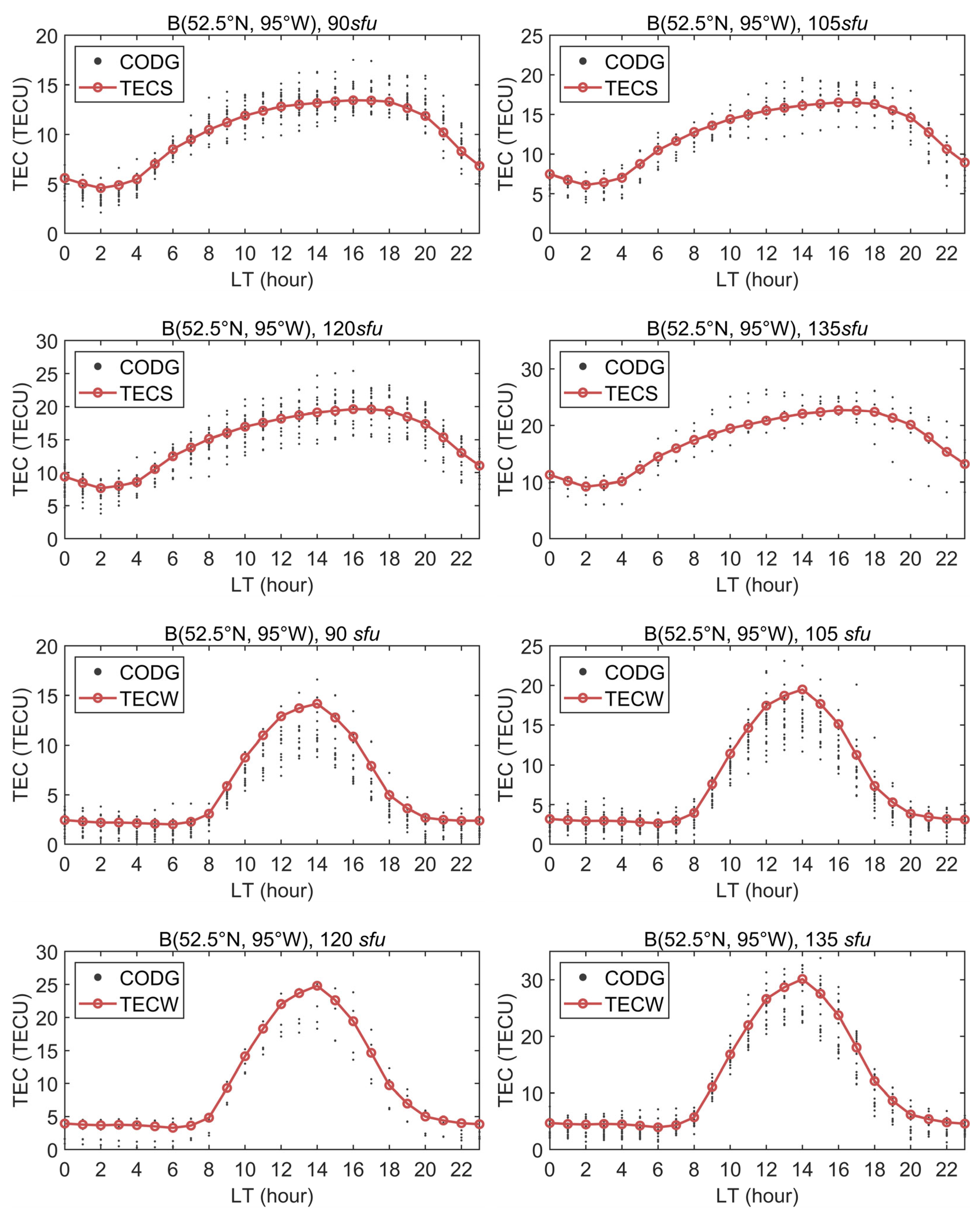
3.1. Viability Analysis
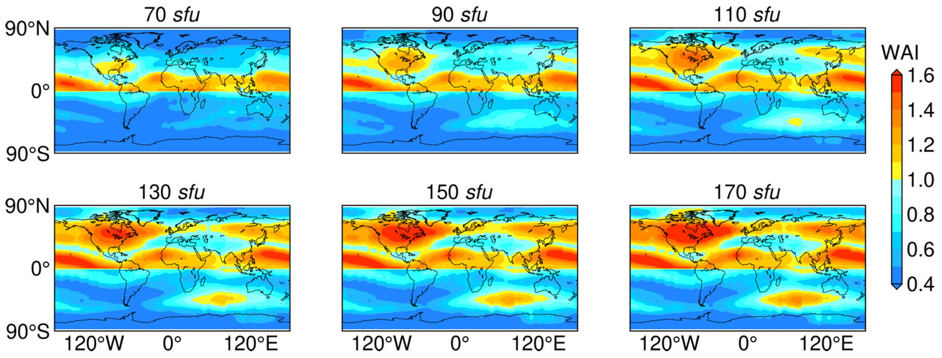
3.2. Winter Anomaly
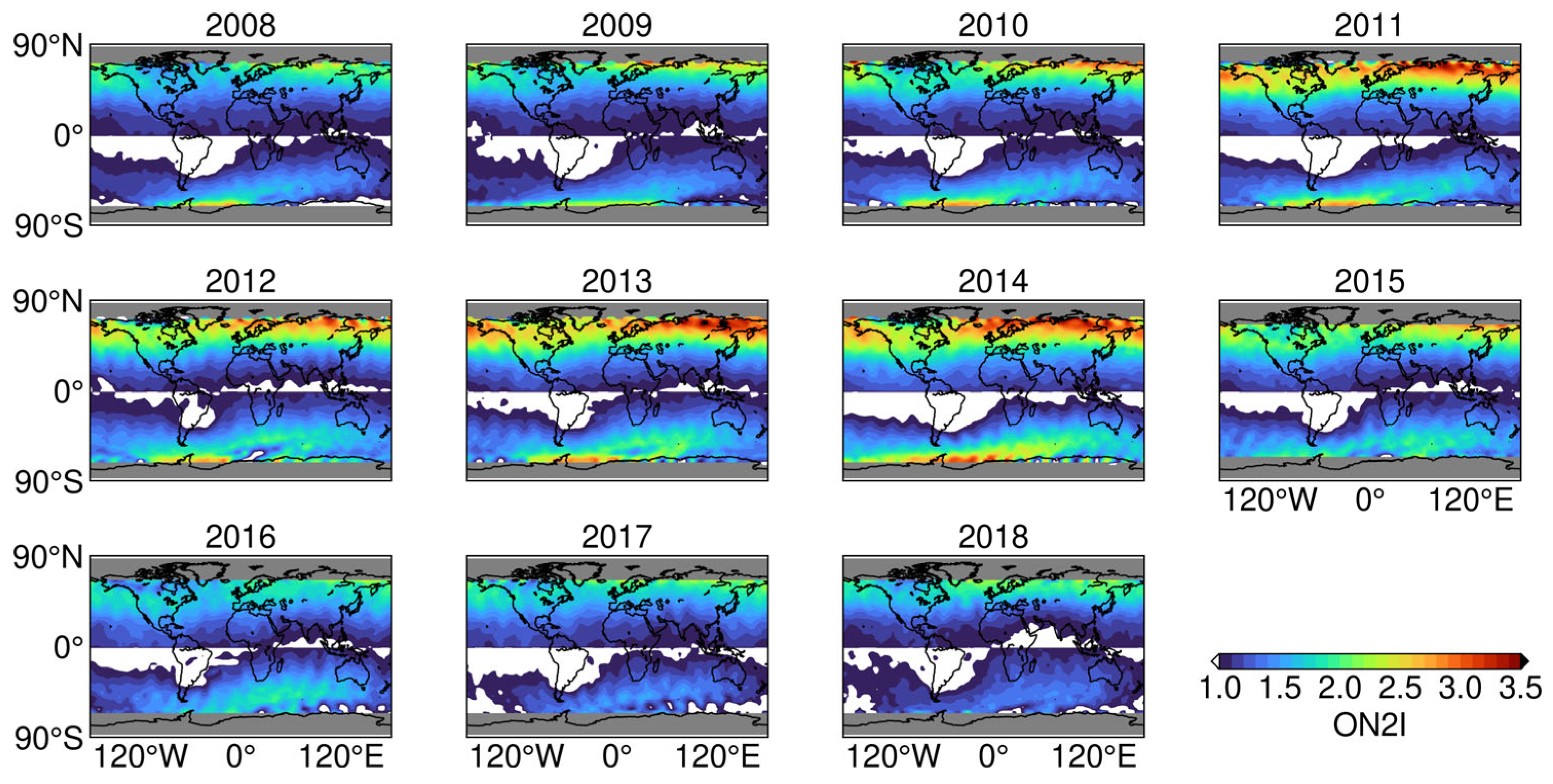
3.3. Annual Anomaly
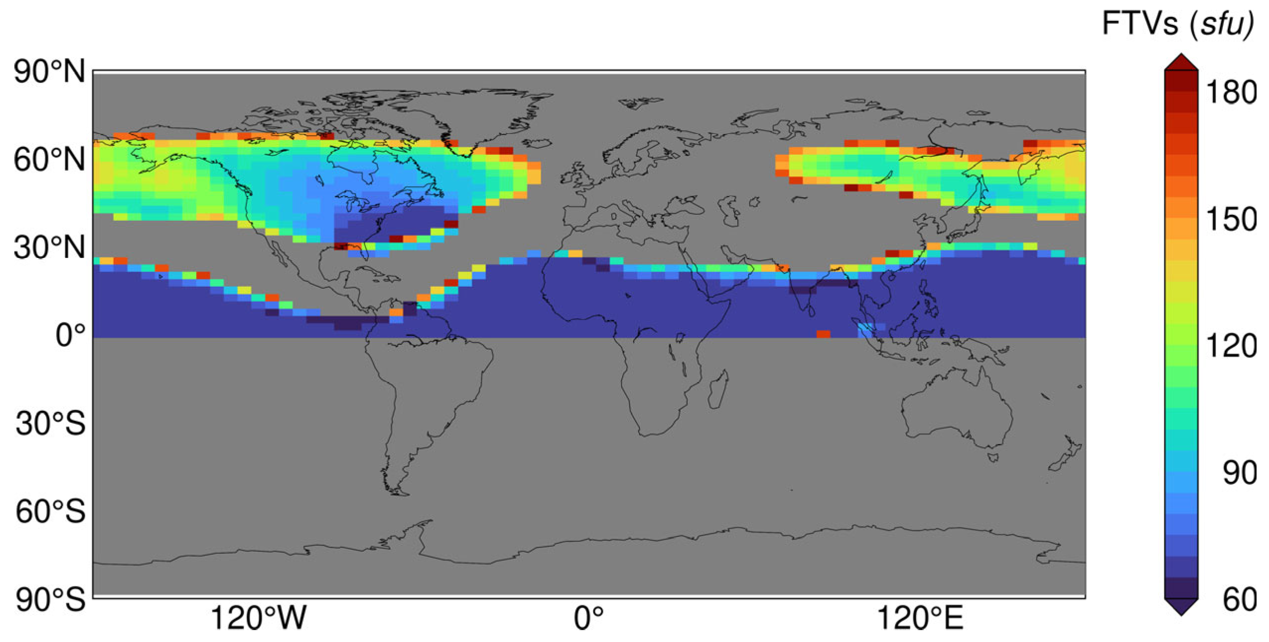
3.4. Contribution of the Winter Anomaly to Annual Anomaly
4. Summary and Conclusions
Author Contributions
Funding
Data Availability Statement
Acknowledgments
Conflicts of Interest
Appendix A
References
- Appleton, E.V.; Naismith, R. Some Further Measurements of Upper Atmospheric Ionization. Proc. R. Soc. Lond. Ser. A Math. Phys. Sci. 1935, 150, 685–708. [Google Scholar] [CrossRef]
- Mendillo, M.; Huang, C.-L.; Pi, X.; Rishbeth, H.; Meier, R. The Global Ionospheric Asymmetry in Total Electron Content. J. Atmos. Sol.-Terr. Phys. 2005, 67, 1377–1387. [Google Scholar] [CrossRef]
- Berkner, L.V.; Wells, H.W. Non-Seasonal Change of F2-Region Ion-Density. Terr. Magn. Atmos. Electr. 1938, 43, 15–36. [Google Scholar] [CrossRef]
- Rishbeth, H. How the Thermospheric Circulation Affects the Ionospheric F2-Layer. J. Atmos. Sol.-Terr. Phys. 1998, 60, 1385–1402. [Google Scholar] [CrossRef]
- Berkner, L.V.; Wells, H.W.; Seaton, S.L. Characteristics of the Upper Region of the Ionosphere. Terr. Magn. Atmos. Electr. 1936, 41, 173–184. [Google Scholar] [CrossRef]
- Appleton, E.V. Two Anomalies in the Ionosphere. Nature 1946, 157, 691. [Google Scholar] [CrossRef]
- Thampi, S.V.; Lin, C.; Liu, H.; Yamamoto, M. First Tomographic Observations of the Midlatitude Summer Nighttime Anomaly over Japan. J. Geophys. Res. Space Phys. 2009, 114, 1–10. [Google Scholar] [CrossRef]
- Torr, M.R.; Torr, D.G. The Seasonal Behaviour of the F2-Layer of the Ionosphere. J. Atmos. Terr. Phys. 1973, 35, 2237–2251. [Google Scholar] [CrossRef]
- Yasyukevich, Y.; Yasyukevich, A.; Ratovsky, K.; Klimenko, M.; Klimenko, V.; Chirik, N. Winter Anomaly in NmF2 and TEC: When and Where It Can Occur. J. Space Weather Space Clim. 2018, 8, A45. [Google Scholar] [CrossRef]
- Azpilicueta, F.; Nava, B. A Different View of the Ionospheric Winter Anomaly. Adv. Space Res. 2021, 67, 150–162. [Google Scholar] [CrossRef]
- Pavlov, A.V.; Pavlova, N.M. Variations in Statistical Parameters of the NmF2 Winter Anomaly with Latitude and Solar Activity. Geomagn. Aeron. 2012, 52, 335–343. [Google Scholar] [CrossRef]
- Zhao, B.; Wan, W.; Liu, L.; Mao, T.; Ren, Z.; Wang, M.; Christensen, A.B. Features of Annual and Semiannual Variations Derived from the Global Ionospheric Maps of Total Electron Content. Ann. Geophys. 2007, 25, 2513–2527. [Google Scholar] [CrossRef]
- Lee, W.K.; Kil, H.; Kwak, Y.-S.; Wu, Q.; Cho, S.; Park, J.U. The Winter Anomaly in the Middle-Latitude F Region during the Solar Minimum Period Observed by the Constellation Observing System for Meteorology, Ionosphere, and Climate. J. Geophys. Res. Space Phys. 2011, 116, 1–10. [Google Scholar] [CrossRef]
- Meza, A.; Natali, M.; Fernandez, L. Analysis of the Winter and Semiannual Ionospheric Anomalies in 1999–2009 Based on GPS Global International GNSS Service Maps. J. Geophys. Res. Space Phys. 2012, 117, 1319. [Google Scholar] [CrossRef]
- Huo, X.L.; Yuan, Y.B.; Ou, J.K.; Zhang, K.F.; Bailey, G.J. Monitoring the Global-Scale Winter Anomaly of Total Electron Contents Using GPS Data. Earth Planets Space 2009, 61, 1019–1024. [Google Scholar] [CrossRef]
- Mikhailov, A.V.; Perrone, L. Comment on “The Winter Anomaly in the Middle-Latitude F Region during the Solar Minimum Period Observed by the Constellation Observing System for Meteorology, Ionosphere, and Climate” by W. K. Lee, H. Kil, Y.-S. Kwak, Q. Wu, S. Cho, and J. U. Park. J. Geophys. Res. Space Phys. 2014, 119, 7972–7978. [Google Scholar] [CrossRef]
- Klimenko, M.V.; Klimenko, V.V.; Zakharenkova, I.E.; Ratovsky, K.G.; Yasyukevich, A.S.; Yasyukevich, Y.V. Altitudinal Extent of Winter Anomaly and Its Manifestation in the Total Electron Content. Russ. J. Phys. Chem. B 2019, 13, 884–891. [Google Scholar] [CrossRef]
- Rishbeth, H.; Setty, C.S.G.K. The F-Layer at Sunrise. J. Atmos. Terr. Phys. 1961, 20, 263–276. [Google Scholar] [CrossRef]
- King, G.A.M. The Dissociation of Oxygen and High Level Circulation in the Atmosphere. J. Atmos. Sci. 1964, 21, 231–237. [Google Scholar] [CrossRef]
- Burns, A.G.; Wang, W.; Qian, L.; Solomon, S.C.; Zhang, Y.; Paxton, L.J.; Yue, X. On the Solar Cycle Variation of the Winter Anomaly. J. Geophys. Res. Space Phys. 2014, 119, 4938–4949. [Google Scholar] [CrossRef]
- Zou, L.; Rishbeth, H.; Müller-Wodarg, I.C.F.; Aylward, A.D.; Millward, G.H.; Fuller-Rowell, T.J.; Idenden, D.W.; Moffett, R.J. Annual and Semiannual Variations in the Ionospheric F2-Layer. I. Modelling. Ann. Geophys. 2000, 18, 927–944. [Google Scholar] [CrossRef]
- Qian, L.; Burns, A.G.; Wang, W.; Solomon, S.C.; Zhang, Y.; Hsu, V. Effects of the Equatorial Ionosphere Anomaly on the Interhemispheric Circulation in the Thermosphere. J. Geophys. Res. Space Phys. 2016, 121, 2522–2530. [Google Scholar] [CrossRef]
- Torr, D.G.; Torr, M.R.; Richards, P.G. Causes of the F Region Winter Anomaly. Geophys. Res. Lett. 1980, 7, 301–304. [Google Scholar] [CrossRef]
- Yonezawa, T. The Solar-Activity and Latitudinal Characteristics of the Seasonal, Non-Seasonal and Semi-Annual Variations in the Peak Electron Densities of the F2-Layer at Noon and at Midnight in Middle and Low Latitudes. J. Atmos. Terr. Phys. 1971, 33, 889–907. [Google Scholar] [CrossRef]
- Rishbeth, H.; Müller-Wodarg, I.C.F.; Zou, L.; Fuller-Rowell, T.J.; Millward, G.H.; Moffett, R.J.; Idenden, D.W.; Aylward, A.D. Annual and Semiannual Variations in the Ionospheric F2-Layer: II. Physical Discussion. Ann. Geophys. 2000, 18, 945–956. [Google Scholar] [CrossRef]
- Rishbeth, H.; Müller-Wodarg, I.C.F. Why Is There More Ionosphere in January than in July? The Annual Asymmetry in the F2-Layer. Ann. Geophys. 2006, 24, 3293–3311. [Google Scholar] [CrossRef]
- Su, Y.Z.; Bailey, G.J.; Oyama, K.-I. Annual and Seasonal Variations in the Low-Latitude Topside Ionosphere. Ann. Geophys. 1998, 16, 974–985. [Google Scholar] [CrossRef]
- Gowtam, V.S.; Ram, S.T. Ionospheric Winter Anomaly and Annual Anomaly Observed from Formosat-3/COSMIC Radio Occultation Observations during the Ascending Phase of Solar Cycle 24. Adv. Space Res. 2017, 60, 1585–1593. [Google Scholar] [CrossRef]
- Rishbeth, H. Thermospheric Targets. Eos Trans. Am. Geophys. Union 2007, 88, 189–193. [Google Scholar] [CrossRef]
- Roma-Dollase, D.; Hernández-Pajares, M.; Krankowski, A.; Kotulak, K.; Ghoddousi-Fard, R.; Yuan, Y.; Li, Z.; Zhang, H.; Shi, C.; Wang, C.; et al. Consistency of Seven Different GNSS Global Ionospheric Mapping Techniques during One Solar Cycle. J. Geod. 2018, 92, 691–706. [Google Scholar] [CrossRef]
- Feng, J.; Wang, K.; Li, W.; Han, B.; Zhao, Z.; Zhang, T.; Meng, D. Analysis of Temporal and Spatial Variation Characteristics of Midlatitude Summer Nighttime Anomaly in Low and Middle Solar Activity Period. Adv. Space Res. 2023, 71, 4351–4360. [Google Scholar] [CrossRef]
- Feng, J.; Han, B.; Zhao, Z.; Wang, Z. A New Global Total Electron Content Empirical Model. Remote Sens. 2019, 11, 706. [Google Scholar] [CrossRef]
- Feng, J.; Yuan, Y.; Zhang, T.; Zhang, Z.; Meng, D. Analysis of Ionospheric Anomalies before the Tonga Volcanic Eruption on 15 January 2022. Remote Sens. 2023, 15, 4879. [Google Scholar] [CrossRef]
- Feng, J.; Zhang, T.; Li, W.; Zhao, Z.; Han, B.; Wang, K. A New Global TEC Empirical Model Based on Fusing Multi-Source Data. GPS Solut. 2022, 27, 20. [Google Scholar] [CrossRef]
- Jakowski, N.; Hoque, M.M.; Mayer, C. A New Global TEC Model for Estimating Transionospheric Radio Wave Propagation Errors. J. Geod. 2011, 85, 965–974. [Google Scholar] [CrossRef]
- Hoque, M.M.; Jakowski, N.; Orús-Pérez, R. Fast Ionospheric Correction Using Galileo Az Coefficients and the NTCM Model. GPS Solut. 2019, 23, 41. [Google Scholar] [CrossRef]
- Schaer, S. Mapping and Predicting the Earth’s Ionosphere Using the Global Positioning System; Institutfür Geodäsie und Photogrammetrie, Eidg, Technische Hochschule Zürich: Zürich, Switzerland, 1999. [Google Scholar]
- Lei, J.; Liu, L.; Wan, W.; Zhang, S.-R. Variations of Electron Density Based on Long-Term Incoherent Scatter Radar and Ionosonde Measurements over Millstone Hill. Radio Sci. 2005, 40, 1–10. [Google Scholar] [CrossRef]
- Alken, P.; Thébault, E.; Beggan, C.D.; Amit, H.; Aubert, J.; Baerenzung, J.; Bondar, T.N.; Brown, W.J.; Califf, S.; Chambodut, A.; et al. International Geomagnetic Reference Field: The Thirteenth Generation. Earth Planets Space 2021, 73, 49. [Google Scholar] [CrossRef]
- Oinats, A.V.; Ratovsky, K.G.; Kotovich, G.V. Influence of the 27-Day Solar Flux Variations on the Ionosphere Parameters Measured at Irkutsk in 2003–2005. Adv. Space Res. 2008, 42, 639–644. [Google Scholar] [CrossRef]


| Year | 2008 | 2009 | 2010 | 2011 | 2012 | 2013 | 2014 | 2015 | 2016 | 2017 | 2018 |
|---|---|---|---|---|---|---|---|---|---|---|---|
| June | 68.3 | 70.9 | 75.9 | 98.2 | 127.8 | 117.5 | 130.5 | 123.0 | 87.1 | 77.3 | 73.2 |
| December | 67.1 | 74.7 | 81.4 | 136.9 | 110.9 | 145.4 | 151.1 | 107.4 | 73.8 | 69.4 | 67.9 |
Disclaimer/Publisher’s Note: The statements, opinions and data contained in all publications are solely those of the individual author(s) and contributor(s) and not of MDPI and/or the editor(s). MDPI and/or the editor(s) disclaim responsibility for any injury to people or property resulting from any ideas, methods, instructions or products referred to in the content. |
© 2023 by the authors. Licensee MDPI, Basel, Switzerland. This article is an open access article distributed under the terms and conditions of the Creative Commons Attribution (CC BY) license (https://creativecommons.org/licenses/by/4.0/).
Share and Cite
Wang, K.; Feng, J.; Zhao, Z.; Han, B. Analysis of Winter Anomaly and Annual Anomaly Based on Regression Approach. Remote Sens. 2023, 15, 4968. https://doi.org/10.3390/rs15204968
Wang K, Feng J, Zhao Z, Han B. Analysis of Winter Anomaly and Annual Anomaly Based on Regression Approach. Remote Sensing. 2023; 15(20):4968. https://doi.org/10.3390/rs15204968
Chicago/Turabian StyleWang, Kaixin, Jiandi Feng, Zhenzhen Zhao, and Baomin Han. 2023. "Analysis of Winter Anomaly and Annual Anomaly Based on Regression Approach" Remote Sensing 15, no. 20: 4968. https://doi.org/10.3390/rs15204968