

Mapping of Mean Deformation Rates Based on APS-Corrected InSAR Data Using Unsupervised Clustering Algorithms

 , , ,
, , ,  , and
, and
Abstract
:1. Introduction
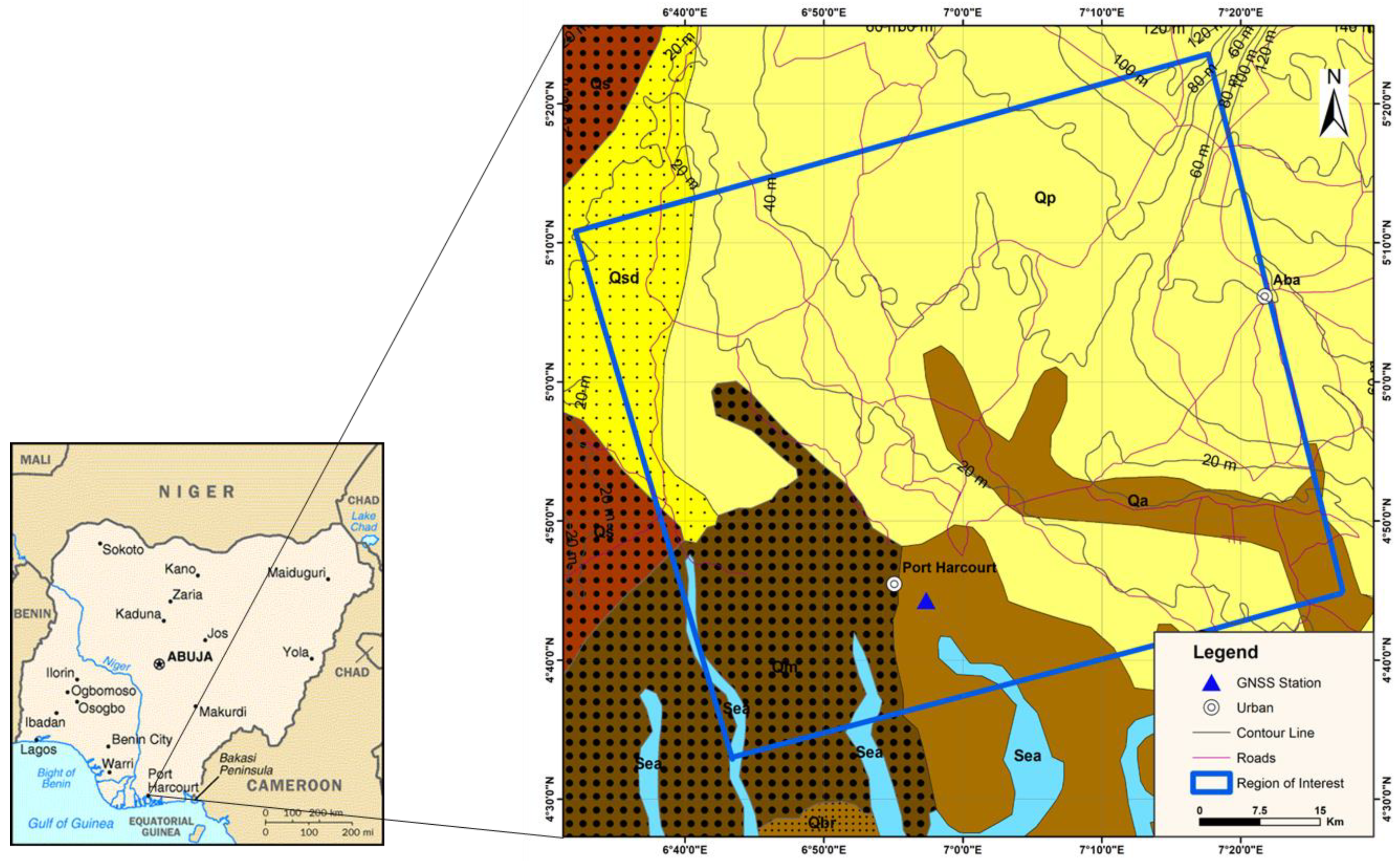
2. Case Study
3. Datasets
4. Methods
4.1. Interferometric Processing
4.1.1. Interferometric SAR (Two-Pass Interferometry, InSAR)
4.1.2. PSI Method
4.1.3. SBAS Method
4.2. Atmospheric Correction on InSAR Signals
Tropospheric Correction Using the AIM
4.3. Data Classification
4.3.1. Unsupervised Clustering
- Exclusive clustering.
- Overlapping clustering.
- 3.
- K-means.
- 4.
- Fuzzy K-means.
- 5.
- K-medians.
K-Means Clustering
K-Medians Clustering
Fuzzy K-Means Clustering
4.4. Evaluation Methods of Clustering Algorithms
4.4.1. Davies–Boldin Index
4.4.2. Similarity Measure
4.5. Satellite Observation Evaluation
5. Results and Validation
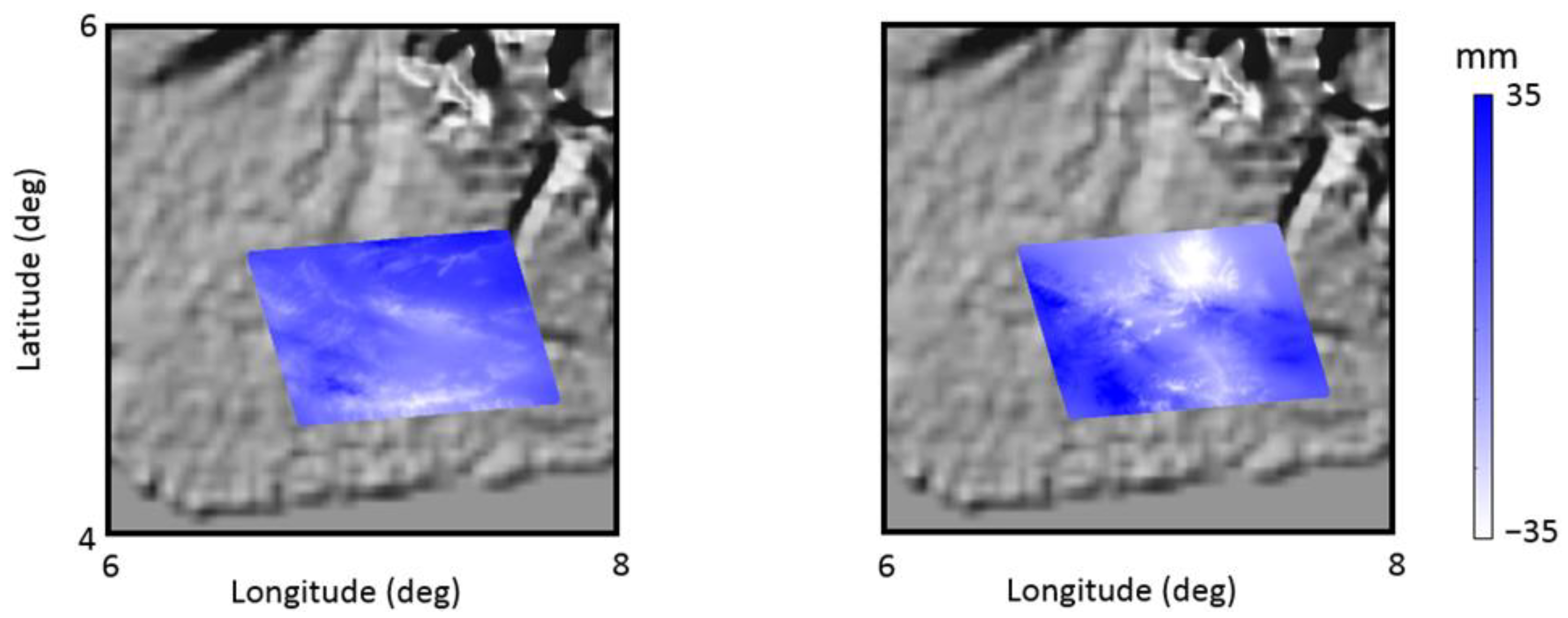
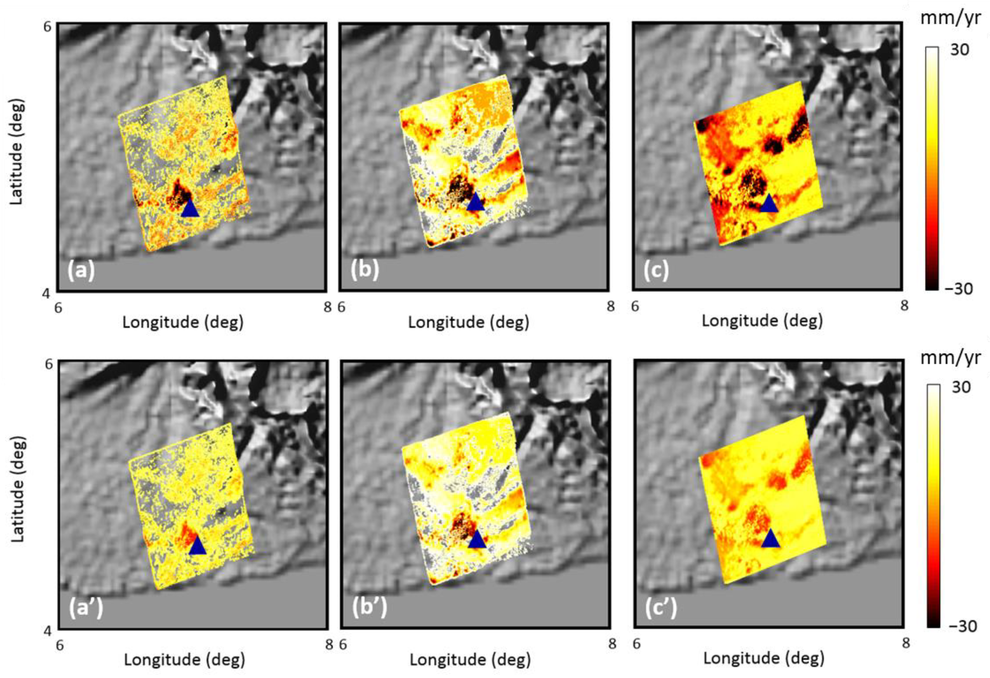
5.1. Subsidence Signals from InSAR Data
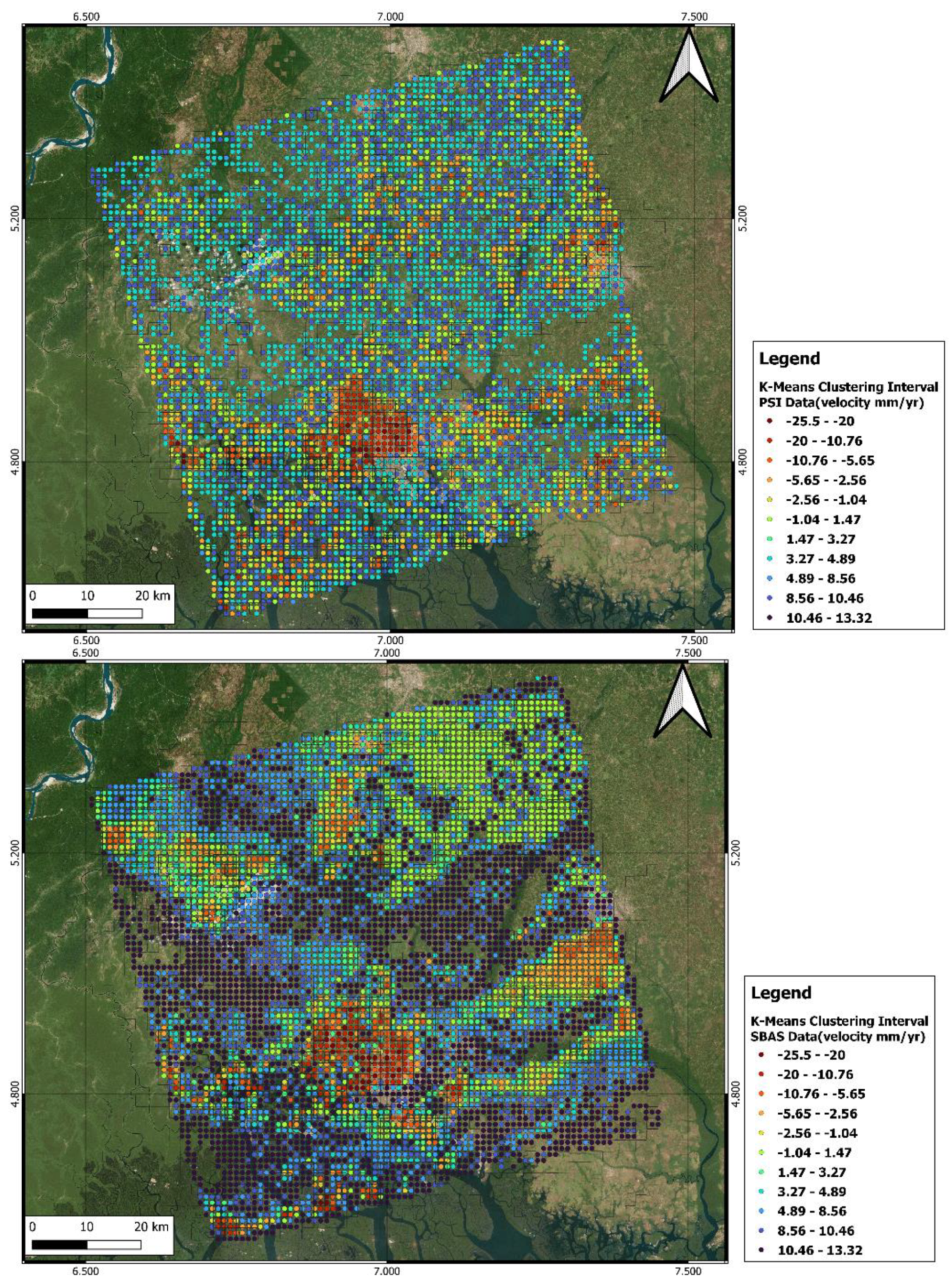
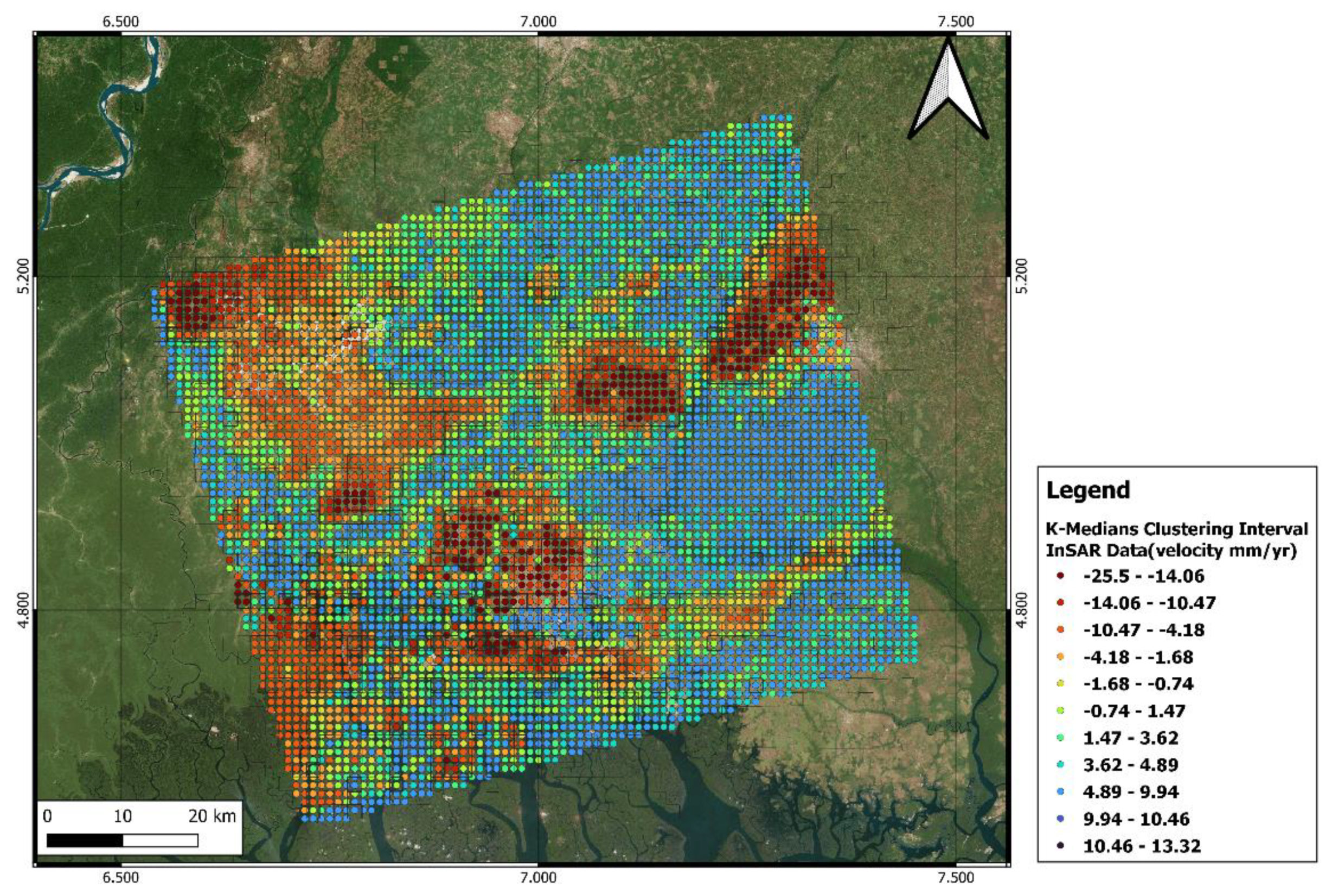
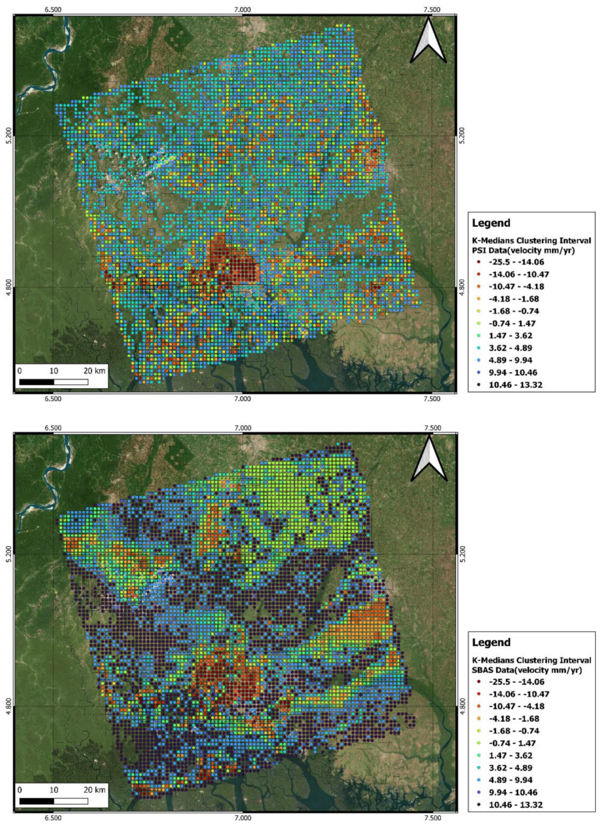
5.2. Classified Subsidence Signals
Unsupervised Clustering
6. Discussion
7. Conclusions
- The AIM for APS correction with ERA5 meteorological data significantly reduced the troposphere and atmospheric delays. One of this paper’s most critical aspects is using the AIM for the first time in three different processing approaches, including SBAS, PSI, and InSAR.
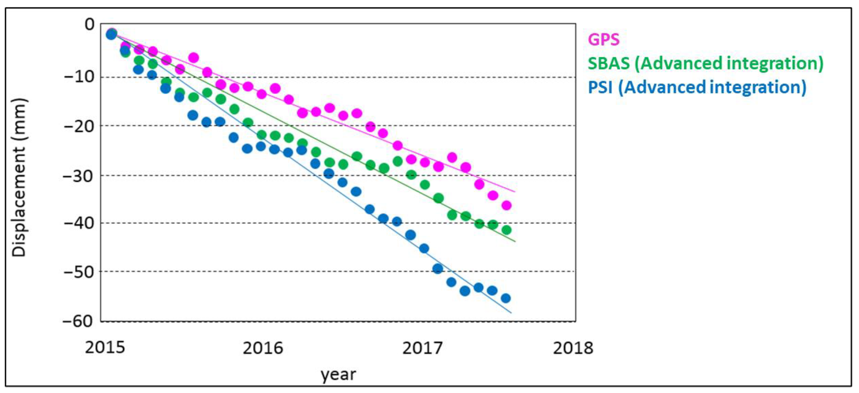
- After implementing the APS correction method for the InSAR, PSI, and SBAS techniques, it was demonstrated that this correction method has improved by 58%, 42%, and 28% for them, respectively, which means that the SBAS technique has created interferograms with higher accuracy during processing in this study area. Additionally, the corrected result value of the SBAS method is consistent and more similar to the vertical component of the GNSS station.
- When the specialists start to process SAR data, they use the intervals of software or packages, either commercial or open source. It is important to emphasize that the MDRMs will change when we use different intervals in the case study. To illustrate reliable deformation parts of the case study, it is essential to identify the best and most accurate intervals based on the case study and deformation zone.
- After choosing the best method with which to find the most reliable and accurate intervals via similarity measures and the DBI, an evaluation of the deformations around the GNSS station within a radius of 500 m was performed. As stated in the Section 4, clustering methods were used to update the points according to latitude, longitude, and velocity. A subsequent analysis of the deformation of the SBAS technique results was conducted without considering the clustering methods, and the same analysis was performed for the SBAS K-medians. Finally, we can observe that the outputs provided by the point position update in clustering methods are 5.5% more accurate than the vertical displacements of the GNSS station.
Author Contributions
Funding
Data Availability Statement
Acknowledgments
Conflicts of Interest
References
- Stramondo, S.; Saroli, M.; Tolomei, C.; Moro, M.; Doumaz, F.; Pesci, A.; Loddo, F.; Baldi, P.; Boschi, E. Surface movements in Bologna (Po Plain—Italy) detected by multitemporal DInSAR. Remote Sens. Environ. 2007, 110, 304–316. [Google Scholar] [CrossRef]
- Bitelli, G.; Bonsignore, F.; Pellegrino, I.; Vittuari, L. Evolution of the techniques for subsidence monitoring at regional scale: The case of Emilia-Romagna region (Italy). Proc. IAHS 2015, 372, 315–321. [Google Scholar] [CrossRef] [Green Version]
- Fiaschi, S.; Tessitore, S.; Bonì, R.; Di Martire, D.; Achilli, V.; Borgstrom, S.; Ibrahim, A.; Floris, M.; Meisina, C.; Ramondini, M.; et al. From ERS-1/2 to Sentinel-1: Two decades of subsidence monitored through A-DInSAR techniques in the Ravenna area (Italy). GISci. Remote Sens. 2017, 54, 305–328. [Google Scholar] [CrossRef]
- Gumilar, I.; Abidin, H.Z.; Hutasoit, L.M.; Hakim, D.M.; Sidiq, T.P.; Andreas, H. Land Subsidence in Bandung Basin and its Possible Caused Factors. Procedia Earth Planet. Sci. 2015, 12, 47–62. [Google Scholar] [CrossRef] [Green Version]
- Coda, S.; Confuorto, P.; De Vita, P.; Di Martire, D.; Allocca, V. Uplift Evidences Related to the Recession of Groundwater Abstraction in a Pyroclastic-Alluvial Aquifer of Southern Italy. Geosciences 2019, 9, 215. [Google Scholar] [CrossRef] [Green Version]
- Coda, S.; Tessitore, S.; Di Martire, D.; Calcaterra, D.; De Vita, P.; Allocca, V. Coupled ground uplift and groundwater rebound in the metropolitan city of Naples (southern Italy). J. Hydrol. 2019, 569, 470–482. [Google Scholar] [CrossRef]
- Valente, E.; Allocca, V.; Riccardi, U.; Camanni, G.; Di Martire, D. Studying a Subsiding Urbanized Area from a Multidisciplinary Perspective: The Inner Sector of the Sarno Plain (Southern Apennines, Italy). Remote Sens. 2021, 13, 3323. [Google Scholar] [CrossRef]
- Foumelis, M.; Papageorgiou, E.; Stamatopoulos, C. Episodic ground deformation signals in Thessaly Plain (Greece) revealed by data mining of SAR interferometry time series. Int. J. Remote Sens. 2016, 37, 3696–3711. [Google Scholar] [CrossRef]
- Baniani, S.R.; Chang, L.; Maghsoudi, Y. Mapping and Analyzing Land Subsidence for Tehran Using Sentinel-1 SAR and GPS and Geological Data. In Proceedings of the EGU General Assembly, Virutal, 19–30 April 2021. [Google Scholar]
- Ghorbani, Z.; Khosravi, A.; Maghsoudi, Y.; Mojtahedi, F.F.; Javadnia, E.; Nazari, A. Use of InSAR data for measuring land subsidence induced by groundwater withdrawal and climate change in Ardabil Plain, Iran. Sci. Rep. 2022, 12, 13998. [Google Scholar] [CrossRef]
- Lazos, I.; Papanikolaou, I.; Sboras, S.; Foumelis, M.; Pikridas, C. Geodetic Upper Crust Deformation Based on Primary GNSS and INSAR Data in the Strymon Basin, Northern Greece—Correlation with Active Faults. Appl. Sci. 2022, 12, 9391. [Google Scholar] [CrossRef]
- Franceschetti, G.; Lanari, R. Synthetic Aperture Radar Processing; CRC Press: Boca Raton, FL, USA, 2018; ISBN 978-0-203-73748-4. [Google Scholar]
- Ferretti, A.; Savio, G.; Barzaghi, R.; Borghi, A.; Musazzi, S.; Novali, F.; Prati, C.; Rocca, F. Submillimeter Accuracy of InSAR Time Series: Experimental Validation. IEEE Trans. Geosci. Remote Sens. 2007, 45, 1142–1153. [Google Scholar] [CrossRef]
- Gabriel, A.K.; Goldstein, R.M.; Zebker, H.A. Mapping small elevation changes over large areas: Differential radar interferometry. J. Geophys. Res. Solid Earth 1989, 94, 9183–9191. [Google Scholar] [CrossRef]
- Ferretti, A.; Prati, C.; Rocca, F. Permanent scatterers in SAR interferometry. IEEE Trans. Geosci. Remote Sens. 2001, 39, 8–20. [Google Scholar] [CrossRef]
- Berardino, P.; Fornaro, G.; Lanari, R.; Sansosti, E. A new algorithm for surface deformation monitoring based on small baseline differential SAR interferograms. IEEE Trans. Geosci. Remote Sens. 2002, 40, 2375–2383. [Google Scholar] [CrossRef] [Green Version]
- Zebker, H.A.; Rosen, P.A.; Hensley, S. Atmospheric effects in interferometric synthetic aperture radar surface deformation and topographic maps. J. Geophys. Res. Solid Earth 1997, 102, 7547–7563. [Google Scholar] [CrossRef]
- Aghajany, S.H.; Voosoghi, B.; Yazdian, A. Estimation of north Tabriz fault parameters using neural networks and 3D tropospherically corrected surface displacement field. Geomat. Nat. Hazards Risk 2017, 8, 918–932. [Google Scholar] [CrossRef] [Green Version]
- Haji-Aghajany, S.; Amerian, Y. Hybrid Regularized GPS Tropospheric Sensing Using 3-D Ray Tracing Technique. IEEE Geosci. Remote Sens. Lett. 2018, 15, 1475–1479. [Google Scholar] [CrossRef]
- Haji-Aghajany, S.; Voosoghi, B.; Amerian, Y. Estimating the slip rate on the north Tabriz fault (Iran) from InSAR measurements with tropospheric correction using 3D ray tracing technique. Adv. Space Res. 2019, 64, 2199–2208. [Google Scholar] [CrossRef]
- Crosetto, M.; Monserrat, O.; Cuevas-González, M.; Devanthéry, N.; Crippa, B. Persistent Scatterer Interferometry: A review. ISPRS J. Photogramm. Remote Sens. 2016, 115, 78–89. [Google Scholar] [CrossRef] [Green Version]
- Jia, H.; Liu, L. A technical review on persistent scatterer interferometry. J. Mod. Transport. 2016, 24, 153–158. [Google Scholar] [CrossRef]
- Pawluszek-Filipiak, K.; Borkowski, A. Integration of DInSAR and SBAS Techniques to Determine Mining-Related Deformations Using Sentinel-1 Data: The Case Study of Rydułtowy Mine in Poland. Remote Sens. 2020, 12, 242. [Google Scholar] [CrossRef] [Green Version]
- Guerriero, L.; Di Martire, D.; Calcaterra, D.; Francioni, M. Digital Image Correlation of Google Earth Images for Earth’s Surface Displacement Estimation. Remote Sens. 2020, 12, 3518. [Google Scholar] [CrossRef]
- Cao, Y.; Jónsson, S.; Li, Z. Advanced InSAR Tropospheric Corrections From Global Atmospheric Models that Incorporate Spatial Stochastic Properties of the Troposphere. J. Geophys. Res. Solid Earth 2021, 126, e2020JB020952. [Google Scholar] [CrossRef]
- Hartigan, J.A.; Wong, M.A. Algorithm AS 136: A K-Means Clustering Algorithm. J. R. Stat. Soc. Ser. C Appl. Stat. 1979, 28, 100–108. [Google Scholar] [CrossRef]
- Jain, A.K.; Dubes, R.C. Algorithms for Clustering Data; Prentice-Hall: Hoboken, NJ, USA, 1988; ISBN 013022278X. [Google Scholar]
- Hung, C.-C.; Kulkarni, S.; Kuo, B.-C. A New Weighted Fuzzy C-Means Clustering Algorithm for Remotely Sensed Image Classification. IEEE J. Sel. Top. Signal Process. 2011, 5, 543–553. [Google Scholar] [CrossRef]
- Assent, I. Clustering high dimensional data. WIREs Data Min. Knowl. Discov. 2012, 2, 340–350. [Google Scholar] [CrossRef]
- Bronstein, M.M.; Bruna, J.; LeCun, Y.; Szlam, A.; Vandergheynst, P. Geometric Deep Learning: Going beyond Euclidean data. IEEE Signal Process. Mag. 2017, 34, 18–42. [Google Scholar] [CrossRef] [Green Version]
- Ruzza, G.; Guerriero, L.; Grelle, G.; Guadagno, F.M.; Revellino, P. Multi-Method Tracking of Monsoon Floods Using Sentinel-1 Imagery. Water 2019, 11, 2289. [Google Scholar] [CrossRef] [Green Version]
- Yu, Y.; Gong, Z.; Zhong, P.; Shan, J. Unsupervised Representation Learning with Deep Convolutional Neural Network for Remote Sensing Images. In Image and Graphics, Proceedings of the 9th International Conference, ICIG 2017, Shanghai, China, 13–15 September 2017; Zhao, Y., Kong, X., Taubman, D., Eds.; Springer International Publishing: Cham, Switzerland, 2017; pp. 97–108. [Google Scholar]
- Nguyen, C.; Starek, M.J.; Tissot, P.; Gibeaut, J. Unsupervised Clustering Method for Complexity Reduction of Terrestrial Lidar Data in Marshes. Remote Sens. 2018, 10, 133. [Google Scholar] [CrossRef] [Green Version]
- Saleem, A. Remote Sensing by using Unsupervised Algorithm. Preprints 2021, 2021070257. [Google Scholar] [CrossRef]
- Van Strien, M.J.; Grêt-Regamey, A. Unsupervised deep learning of landscape typologies from remote sensing images and other continuous spatial data. Environ. Model. Softw. 2022, 155, 105462. [Google Scholar] [CrossRef]
- Yalvac, S. Validating InSAR-SBAS results by means of different GNSS analysis techniques in medium- and high-grade deformation areas. Environ. Monit. Assess. 2020, 192, 120. [Google Scholar] [CrossRef]
- Kinnaird, P.B.J.A. Geology and Mineralization of the Nigerian Anorogenic Ring Complexes; Schweizerbart Science Publishers: Stuttgart, Germany, 1984; ISBN 978-3-510-96289-1. [Google Scholar]
- Odigi, M.I.; Amajor, L.C. Brittle deformation in the Afikpo Basin (Southeast Nigeria): Evidence for a terminal Cretaceous extensional regime in the Lower Benue Trough, Nigeria. Chin. J. Geochem. 2009, 28, 369. [Google Scholar] [CrossRef]
- Ananaba, S.E.; Ajakaiye, D.E. Evidence of tectonic control of mineralization in Nigeria from lineament density analysis A Landsat-study. Int. J. Remote Sens. 1987, 8, 1445–1453. [Google Scholar] [CrossRef]
- Jimoh, A.Y.; Ojo, O.J.; Akande, S.O. Organic petrography, Rock–Eval pyrolysis and biomarker geochemistry of Maastrichtian Gombe Formation, Gongola Basin, Nigeria. J. Pet. Explor. Prod. Technol. 2020, 10, 327–350. [Google Scholar] [CrossRef] [Green Version]
- Odigi, M.I.; Amajor, L.C. Geochemical characterization of Cretaceous sandstones from the Southern Benue Trough, Nigeria. Chin. J. Geochem. 2009, 28, 44–54. [Google Scholar] [CrossRef]
- Hersbach, H.; Bell, B.; Berrisford, P.; Hirahara, S.; Horányi, A.; Muñoz-Sabater, J.; Nicolas, J.; Peubey, C.; Radu, R.; Schepers, D.; et al. The ERA5 global reanalysis. Q. J. R. Meteorol. Soc. 2020, 146, 1999–2049. [Google Scholar] [CrossRef]
- Longuevergne, L.; Wilson, C.R.; Scanlon, B.R.; Crétaux, J.F. GRACE water storage estimates for the Middle East and other regions with significant reservoir and lake storage. Hydrol. Earth Syst. Sci. 2013, 17, 4817–4830. [Google Scholar] [CrossRef] [Green Version]
- Tourian, M.J.; Elmi, O.; Chen, Q.; Devaraju, B.; Roohi, S.; Sneeuw, N. A spaceborne multisensor approach to monitor the desiccation of Lake Urmia in Iran. Remote Sens. Environ. 2015, 156, 349–360. [Google Scholar] [CrossRef]
- Dahri, Z.H.; Ludwig, F.; Moors, E.; Ahmad, S.; Ahmad, B.; Shoaib, M.; Ali, I.; Iqbal, M.S.; Pomee, M.S.; Mangrio, A.G.; et al. Spatio-temporal evaluation of gridded precipitation products for the high-altitude Indus basin. Int. J. Climatol. 2021, 41, 4283–4306. [Google Scholar] [CrossRef]
- Hanssen, R.F. Radar Interferometry: Data Interpretation and Error Analysis; Springer Science & Business Media: Berlin/Heidelberg, Germany, 2001; ISBN 978-0-7923-6945-5. [Google Scholar]
- Hooper, A. A multi-temporal InSAR method incorporating both persistent scatterer and small baseline approaches. Geophys. Res. Lett. 2008, 35, L16302. [Google Scholar] [CrossRef] [Green Version]
- Hooper, A.; Zebker, H.; Segall, P.; Kampes, B. A new method for measuring deformation on volcanoes and other natural terrains using InSAR persistent scatterers. Geophys. Res. Lett. 2004, 31, L23611. [Google Scholar] [CrossRef]
- Gray, A.L.; Mattar, K.E.; Sofko, G. Influence of ionospheric electron density fluctuations on satellite radar interferometry. Geophys. Res. Lett. 2000, 27, 1451–1454. [Google Scholar] [CrossRef]
- Hanssen, R.F. Atmospheric Heterogeneities in ERS Tandem SAR Interferometry; Delft University Press: Delft, The Netherlands, 1998. [Google Scholar]
- Jolivet, R.; Agram, P.S.; Lin, N.Y.; Simons, M.; Doin, M.-P.; Peltzer, G.; Li, Z. Improving InSAR geodesy using Global Atmospheric Models. J. Geophys. Res. Solid Earth 2014, 119, 2324–2341. [Google Scholar] [CrossRef]
- Chen, C.W.; Zebker, H.A. Phase unwrapping for large SAR interferograms: Statistical segmentation and generalized network models. IEEE Trans. Geosci. Remote Sens. 2002, 40, 1709–1719. [Google Scholar] [CrossRef] [Green Version]
- Dee, D.P.; Uppala, S.M.; Simmons, A.J.; Berrisford, P.; Poli, P.; Kobayashi, S.; Andrae, U.; Balmaseda, M.A.; Balsamo, G.; Bauer, P.; et al. The ERA-Interim reanalysis: Configuration and performance of the data assimilation system. Q. J. R. Meteorol. Soc. 2011, 137, 553–597. [Google Scholar] [CrossRef]
- Ahuja Greenlaw, R.; Kantabutra, S. Introduction to Clustering. In Dynamic and Advanced Data Mining for Progressing Technological Development; IGI Global: Hershey, PA, USA, 2010; pp. 224–254. [Google Scholar]
- Bezdek, J.C. Cluster Validity. In Pattern Recognition with Fuzzy Objective Function Algorithms; Advanced Applications in Pattern Recognition; Bezdek, J.C., Ed.; Springer: Boston, MA, USA, 1981; pp. 95–154. ISBN 978-1-4757-0450-1. [Google Scholar]
- Jiang, D.; Tang, C.; Zhang, A. Cluster analysis for gene expression data: A survey. IEEE Trans. Knowl. Data Eng. 2004, 16, 1370–1386. [Google Scholar] [CrossRef]
- Pearson, K. Contributions to the Mathematical Theory of Evolution. Philos. Trans. R. Soc. London. A 1894, 185, 71–110. [Google Scholar]
- Ikuemonisan, F.E.; Ozebo, V.C. Characterisation and mapping of land subsidence based on geodetic observations in Lagos, Nigeria. Geod. Geodyn. 2020, 11, 151–162. [Google Scholar] [CrossRef]


| Mission | Acquisition Time (Images) | Product | Path | Swath | Pass | Central Look Angle (Deg) | Polarization |
|---|---|---|---|---|---|---|---|
| Sentinel-1A | 2015 to 2017 (37) | Single-look complex (SLC) | 103 | IW TOPS | Ascending | 38° | VV |
| SAR Processing Approaches at the Specific Point Near the GNSS Station | Velocity (mm/yr) before APS Correction | Velocity (mm/yr) after APS Correction | The Percentage of Improvement |
|---|---|---|---|
| SBAS | −27.7 | −20.3 | 28% |
| PSI | −47.0 | −27.3 | 42% |
| InSAR | −80.2 | −33.7 | 58% |
| InSAR Processing Techniques with Three Clustering Methods | DBI |
|---|---|
| InSAR technique with fuzzy clustering | 0.535586 |
| PSI technique with fuzzy clustering | 0.454458 |
| SBAS technique with fuzzy clustering | 0.478788 |
| InSAR technique with K-means clustering | 0.513885 |
| PSI technique with K-means clustering | 0.443950 |
| SBAS technique with K-means clustering | 0.438856 |
| InSAR technique with K-medians clustering | 0.569536 |
| PSI technique with K-medians clustering | 0.493579 |
| SBAS technique with K-medians clustering | 0.397198 |
| InSAR Processing Techniques with Three Clustering Methods | Accuracy |
|---|---|
| InSAR technique with fuzzy clustering | 0.8645 |
| PSI technique with fuzzy clustering | 0.8649 |
| SBAS technique with fuzzy clustering | 0.8954 |
| InSAR technique with K-means clustering | 0.8736 |
| PSI technique with K-means clustering | 0.8497 |
| SBAS technique with K-means clustering | 0.8984 |
| InSAR technique with K-medians clustering | 0.8796 |
| PSI technique with K-medians clustering | 0.8826 |
| SBAS technique with K-medians clustering | 0.9146 |
| Method | Similarity with GNSS Station |
|---|---|
| SBAS | 89% |
| SBAS technique with K-medians clustering | 94.5% |
Disclaimer/Publisher’s Note: The statements, opinions and data contained in all publications are solely those of the individual author(s) and contributor(s) and not of MDPI and/or the editor(s). MDPI and/or the editor(s) disclaim responsibility for any injury to people or property resulting from any ideas, methods, instructions or products referred to in the content. |
© 2023 by the authors. Licensee MDPI, Basel, Switzerland. This article is an open access article distributed under the terms and conditions of the Creative Commons Attribution (CC BY) license (https://creativecommons.org/licenses/by/4.0/).
Share and Cite
Khalili, M.A.; Voosoghi, B.; Guerriero, L.; Haji-Aghajany, S.; Calcaterra, D.; Di Martire, D. Mapping of Mean Deformation Rates Based on APS-Corrected InSAR Data Using Unsupervised Clustering Algorithms. Remote Sens. 2023, 15, 529. https://doi.org/10.3390/rs15020529
Khalili MA, Voosoghi B, Guerriero L, Haji-Aghajany S, Calcaterra D, Di Martire D. Mapping of Mean Deformation Rates Based on APS-Corrected InSAR Data Using Unsupervised Clustering Algorithms. Remote Sensing. 2023; 15(2):529. https://doi.org/10.3390/rs15020529
Chicago/Turabian StyleKhalili, Mohammad Amin, Behzad Voosoghi, Luigi Guerriero, Saeid Haji-Aghajany, Domenico Calcaterra, and Diego Di Martire. 2023. "Mapping of Mean Deformation Rates Based on APS-Corrected InSAR Data Using Unsupervised Clustering Algorithms" Remote Sensing 15, no. 2: 529. https://doi.org/10.3390/rs15020529