Article

Tree Species Classification Using Airborne LiDAR Data Based on Individual Tree Segmentation and Shape Fitting

School of Remote Sensing and Information Engineering, Wuhan University, Wuhan 430070, China
*
Author to whom correspondence should be addressed.
These authors contributed equally to this work.
Remote Sens. 2023, 15(2), 406; https://doi.org/10.3390/rs15020406
Submission received: 3 December 2022 / Revised: 29 December 2022 / Accepted: 3 January 2023 / Published: 9 January 2023
(This article belongs to the Special Issue 3D Point Clouds in Forest Remote Sensing II)

Abstract

:
Individual tree species classification is of strategic importance for forest monitoring, analysis, and management, which are critical for sustainable forestry development. In this regard, the paper proposes a method based on the profile of segmented individual tree laser scanning points to identify tree species. The proposed methodology mainly takes advantage of three-dimensional geometric features of a tree crown captured by a laser point cloud to identify tree species. Firstly, the Digital Terrain Model (DTM) and Digital Surface Model (DSM) are used for Crown Height Model (CHM) generation. Then, local maximum algorithms and improved rotating profile-based delineations are used to segment individual trees from the profile CHM point data. In the next step, parallel-line shape fitting is used to fit the tree crown shape. In particular, three basic geometric shapes, namely, triangle, rectangle, and arc are used to fit the tree crown shapes of different tree species. If the crown belongs to the same crown shape or shape combination, parameter classification is used, such as the ratio of crown width and crown height or the apex angle range of the triangles. The proposed method was tested by two real datasets which were acquired from two different sites located at Tiger and Leopard National Park in Northeast China. The experimental results indicate that the average tree classification accuracy is 90.9% and the optimal classification accuracy reached 95.9%, which meets the accuracy requirements for rapid forestry surveying.

1. Introduction

Tree species information is a basic parameter in vegetation monitoring, change detection, forest inventory, tree growth condition analyzing, and carbon stock predicting, to mention only a few [1,2,3,4,5]. In sustainable forest management, spatial and structure information of individual trees offer crucial information for management decisions.
Tree species classification originally relied on expensive and time-consuming field investigations to measure structure attributes such as tree height, leaf area index, branch angle etc. of individual trees, then identified the tree species by comparing these parameters to a standard one, where visual inspection by a botanist is usually necessary [6]. With the development of the remote sensing technique, large-scale classification of tree species became possible. Most studies conducted in the past two decades tried to enhance the performance of extraction of structure parameters of individual trees from both optical and Synthetic Aperture Radar (SAR) images, then input them into a classifier to identify each individual tree species [7,8]. Some earlier research also tried to establish the statistical, physical, and geometric relationships between electromagnetic scattering characteristics of various tree species and parameters of interest [9], leading to the intensive study of forest parameters retrieval, such as biomass, leaf and basal area, net and gross primary production (NPP/GPP), etc. [8,10,11,12,13,14] from remote sensing data. The existing studies show that conventional optical remote sensing data are applicable for large-scale forest monitoring and classification, because tree components such as water and chlorophyll show strong absorption in the visible and infrared spectral bands [15,16]. Many machine learning methods have been developed for pixel-level classification based on spectral differences among tree species, which are generally caused by their differences in foliar properties [17,18,19]. SAR data, especially in L-band or P-band, have showed superiority in small scale forest monitoring and species identification due to its penetrability of the tree canopy [20,21,22,23], But the inherent speckle noises in SAR data pose huge challenges for extracting fine structural information from them, and it is difficult to use SAR data alone for accurate classification of tree species [24]. As a result, for large-scale tree species identification, it is difficult, if not impossible, to extract structural information on individual trees from SAR data.
Airborne LiDAR is another kind of active remote sensing technique developed in the early 1960s using pulsed lasers to detect and measure terrain and object surfaces, providing range data in the form of three-dimensional point clouds [25,26]. The application of LiDAR data in forest inventory began in the early 1980s [27], though it had already been employed to generate the Digital Elevation Model (DEM) [28], because it acquires high precision 3D coordinate values of the Earth’s surface. Most research on tree species classification using airborne LiDAR data pays the most attention to the extraction of structural parameters from the data, for example, Holmgren and Persson [29] classified Norway spruce and Scotch Pine with an overall accuracy of 95%, which applied tree height and average forest plot height, such as Lorey’s mean height, and predominant tree height extracted from laser scanning point clouds put to supervised classifiers. In this aspect, differences in the definitions of tree structure parameters can change the classification accuracy [30]. For instance, mean tree height may be taken as the average height of dominant and co-dominant trees [31], whereas others may consider the contribution from suppressed trees [32,33,34].
Full waveform LiDAR data, which can be acquired by installing a full waveform digitizer to the traditional discrete LiDAR system, provide a higher point density and additional information about the vertical characteristics of a tree which has been proved to apply to tree species classification [35,36,37]. Some attempts were made to fully use the structure information of the tree canopy for species classification, which needs to decompose the waveform data to obtain the high-density point cloud data and to retrieve the more vertical structure information of individual tree crowns, e. g., Riaño, Reitberger et al. [34,38]. However, full waveform decomposition is complex and time-consuming, and different decomposition algorithms may achieve different parameters, which hinder their application to large scale tree species classification.
Accuracy can be improved by using the LiDAR intensity values through a multiple band LiDAR system [39], both for individual tree segmentation and tree species classification [40,41,42,43,44,45,46,47,48,49,50,51], two main aspects in terms of applying LiDAR data for automatic forest inventory. For example, Sooyoung Kim et al. in 2009 [47] and 2011 [52] employed the mean intensity values of individual tree crowns to identify the leaf-on and leaf-off tree species; also, Reitberger et al. [38] applied supervised and unsupervised classification to classify fir and spruce by combining intensity values with other attributes from full waveform LiDAR data. Other strategies to improve both segmentation and classification accuracy include point clouds and spectral image fusion, and the application of recently developed machine learning algorithms such as deep neural networks [42,43]. Though promising experimental results were achieved, the former largely depended on the registration accuracy of point clouds and image data, while the latter required a large quantity of training samples.
Based on the above, the classification and recognition of tree species based on remote sensing technology has been highly developed, which enables determination of the key driving factors affecting forest biomass from complex predictors to obtain the quantitative estimation of above ground biomass [53,54]. Also, some tree species results from LiDAR points have been successfully applied to cultivated or invasive tree species above ground biomass estimation [55,56,57,58].
However, in summary, tree species classification based on remotely sensed data still shows the following challenges:
(1) It is difficult to obtain tree structure information by solely using optical images or SAR data, hence it is not easy to achieve high accuracy tree species classification at the crown level.
(2) More precise tree structure information can be retrieved from full waveform data than from the point cloud, but the identification results rely heavily on the precision of waveform decomposition. Moreover, to acquire full waveform data, more budget and more storage resources are required.
(3) The LiDAR point cloud shows promising results in terms of tree species identification by the parameters describing the structural information of tree crowns. However, the parameters depend on the quality of the point cloud in general, and the point cloud density in particular. A better strategy for accurate tree species identification or classification requires the integration of structural and spectral information from the optical images and point cloud, respectively.
Bearing the above-mentioned challenges in mind, the paper attempts to match the segmented tree crown with specific geometric shapes, that is, based on the extraction of the outer contour of a tree crown, a specific shape or the combination of several shapes are used to represent it to avoid the impact of point cloud density on the tree species classification. After the crown segmentation, it is possible to select a limited number of basic shapes, namely triangles, rectangles, or arcs as the basic geometric elements to fit the tree crown shape. If the crown shape is relatively complex, a combination of basic shapes will be adopted to fit it. Then, if the crown belongs to the same type of shape, parameter classification, which completely transforms the crown into relative structure parameters to eliminate the influence of the tree size and the density of the point cloud, is used. The developed method showed a high accuracy of 90.9% in individual tree species classification by using the two test datasets acquired from two sites in Northeastern China.

2. Data and Method

2.1. Data

2.1.1. Study Site

Northeast Hupao National Park is located in the southern area of Laoyeling at the junction of Jilin and Heilongjiang provinces, with a total area of 14,612 square kilometers. Among them, Jilin province accounted for 69.41% and Heilongjiang accounted for 30.59%.
Northeast Hupao National Park is located in the center of the temperate coniferous and broad-leaved mixed forest ecosystem in Asia, containing extremely rich temperate forest plant species in the park. The soil is mainly dark brown soil and marshland, belonging to the continental humid monsoon climate area, with a forest coverage of 92.94%.
From Figure 1, sample plots of diameters of 30 m were set up in the survey area of Northeast Hupao National Park, which mainly includes five types of trees, including Pine, Birch, Cedar, Tsubaki, and Shrub. Then, ten sample plots were selected to test the algorithm, which contains various origins, terrains, and slope directions that meet the test requirements of DTM acquisition, tree crown segmentation, tree location, and finally, tree species classification.

2.1.2. LiDAR Data

Airborne laser point cloud data are carried out by an airborne lidar scanning system, combined with IMU/DGPS assisted aerial measurement technology. Specifically, a Cessna 208b aircraft is selected to carry a riegl-vq-1560i lidar load (seamless integration of inertial navigation IMU and GNSS system). The Cessna 208b aircraft is also observed and obtained jointly with the ground CORS station and artificial base station. The flight height of LiDAR data acquiring is set at an average of 1000 m above ground level (AGL), and the laser records four returns per laser pulse. With a 20% overlap of flight lines, the average laser point density is 20 ppm2. The reported horizontal accuracy is 15 to 25 cm, and vertical accuracy is about 15 cm for the mission specifications of this project. And all the details are listed in Table 1.

2.2. Methods

2.2.1. Procedure Instruction

Figure 2 shows the framework applied by our algorithms. The only input to the algorithm is the raw LiDAR points data. First of all, the TIN filtering method is used to get the terrain points, and the high vegetation points can be extracted by using height from the ground, which returns information. Secondly, we developed a new method designed to acquire the priori information required by a rotating profile analysis algorithm (RPAA). Finally, the section profile method works for extracting the basic shape characteristics of the segmented tree crowns. In addition, a parallel-line shape fitting method is used for fitting the tree crown shapes to the basic geometrical shapes or the combination of shapes and to classify the tree species.

2.2.2. The DEM Generation

Point cloud filtering is the process of separating ground points and non-ground points in the airborne LiDAR point cloud data. The obtained ground points can generate a DEM. Triangulated Irregular Network progressive adaptive filtering algorithm is a universal algorithm which was first proposed by Axelsson [59]. As the Figure 3 shows, the algorithm first selects the initial seed point to construct an initial TIN, and then gradually judges and adds other points to the ground points. The criteria are the angle and vertical distance from this point to the original triangular plane. When the angle and vertical distance are both less than the set thresholds, the point is classified as a ground point. The specific steps of the algorithm are as follows:
  • Selection of initial seed points. The ten plots in this study are all forest plots without buildings, so the default value of 20 m is used as the grid length to divide, and the lowest elevation point in each grid is taken as the starting seed point for the algorithm.
  • Construction of a triangulation network. Use of the starting seed point to construct a sparse TIN as the initial triangulation.
  • Iterative processing. In a certain iteration, judge the points one by one based on the initial triangulation. Take point P as an example: calculate the distance from P to the TIN and the maximum angle between the three vertices of the triangle; if both are within the set threshold ranges, mark P as a ground point and add it to the TIN (otherwise P is classified as a non-ground point). Repeat this process until all points that meet the threshold conditions are classified as ground points. The next iteration obtains new ground points until no more points meet the threshold conditions and the iteration stops.
The experimental results show that the filtering algorithm based on the irregular triangle network has fewer iterations and performs well for most terrain data.

2.2.3. The Normalized Tree Points (NTP)

The elevation value of the airborne LiDAR point cloud data is the superposition of the ground object elevation value and the ground elevation value. In forestry applications, if the terrain causes the tall vegetation on the lowland to undulate greatly, the terrain will have a higher elevation value than the low vegetation on the highland, which makes the elevation value of the LiDAR point cloud data unable to directly reflect the true height of vegetation. Therefore, it is usually necessary to normalize the LiDAR data for the vegetation related research.
Point cloud normalization refers to subtracting the elevation value of the DEM, which is generated by the denoised point cloud. The normalized LiDAR point cloud data can eliminate the influence of the terrain; then the highest single tree point obtained after segmentation can be approximated as the tree height. In this process, the software LiDARMate is used to get the normalized tree points.

2.2.4. Rough Location of Trees

The normalized tree points CNTP are used to derive the tree locations by pinpointing the treetop points which are literally scattered on top among the trees.
Grids derived from points cluster CNTP are required. The size of each grid cell depends on the average distance d ¯ between terrain points, as shown in (1). All tree points are divided into grids accordingly and a a certain value to each grid (GV) via the following formula:
W g r i d = k d ¯   ,   k > 0
G V = { 0 ,                               m = 0 max ( Z N T P i ) ,           m 1 ,   i = 1 ,   2 ,   3 , , m
where
  • GV: the value of the grid cell
  • m: he tree point amount in one grid
  • ZNTP: the Z value of the tree points
The cell containing the treetop point should have the biggest value among the eight neighboring cells, and the top point at center should not be adjacent to any grid without tree points. The template in (2) is applied to derive the treetop grids GVtop. Among all the GVtop, the point with the biggest value is regarded as the initial treetop point Ptop, and every point Ptop in the grids is clustered as point set of CPtop .
T = [ 1 1 1 1 8 1 1 1 1 ]
H ( G V ) = T · G V
{ H ( G V ) i j     G V t o p                     H ( G V ) i j > H T     p     C p t o p                                           Z p = max ( Z p t )  
where
  • T: the convolution template
  • GV: the Z value of the current gird
  • H (GV): judgement value for treetop
  • HT: threshold value of H(GV)
  • p: certain tree point in current grid
  • Zp, Zpt: Z value of the point
In the case of missing small treetops, the size of the grid cell is condensed into an acceptable small range, which results in redundancy in that there are some small treetops belonging to their neighboring tall tree (see Figure 4). Assuming that the tree top point stands for the tree location, the point set CPtop is lowered by the Z value, according to the symmetric structure of trees, and the treetop point can be seen as the center of the tree trunk.
To percolate the fake treetop points, Formula (6) is used. Once treetop points are refined, the number of points is exactly the number of trees.
{ max ( P i   ,   P i + 1     ) C t o p ,                   P i   P i + 1     < D                       P i   ,   P i + 1     C t o p ,     P i   P i + 1     > D
where
  • D: threshold distance of two treetops.
From Figure 4, the distance between the p1, p2, and p2, p3 are both less than threshold D, but p1 is taller than p3, so p2 will be merged with p1 and that is in line with the fact that the taller the tree is, the larger the crown will be.
In this section, all the tree locations can be detected, including the false ones, because the template calculation is more sensitive to elevation fluctuations. As Figure 5 shows, in one tree, there may be multiple treetops. And the Figure 6 shows the process of obtaining original treetop points.

2.2.5. Extraction of the Individual Tree

In this section, the rotating profile is used to segment the tree points and refine the tree locations simultaneously as Figure 7 shows. Section profiles differ with different directions. To identify individual trees precisely, the parameters can be extracted by analyzing a series of rotating pieces of profile information at a certain angle (RPAA), with the steps detailed below:
(1) Descend the treetop points Ctop by Z value. The first point P with the biggest Z value is defined as the highest tree in the test site.
(2) Given a Ptop, get a certain profile with rotation angle. Then divide the section profile into N sub-segments, set Zt as the maximum Z of the point Pt of tree points in sub-segment St ( 0   t N ). From both sides of the St, find out the point Pedge and the point Pcross (see Figure 8 and formula [7]).
(3) Rotate the profile to another angle around the Ptop and get the new point Pedge and the point Pcross and repeat rotating profiles until the rotating angle reaches 180° and all the possible edge points of trees can be obtained and get the coarse range Rt of the trees.
(4) Traverse the remaining treetops; if some fall within the Rt, remove those treetop points from the Ctop. All the high vegetation points within the scope Rt can be classified into the tree cluster segment with treetop of Ptop.
(5) Repeat 1–4, until all the treetops finish the points cluster segment.
(6) The remaining high vegetation points can be grouped into corresponding segmented tree crown points set using the shortest distance (ds) to the tree’s central axis. Where the tree’s central axis is a straight line from the center of the canopy point of gravity to the ground, and the ds is less than the threshold Dmax, which can exclude some isolated high vegetation points.
P t i = {   P e d g e     ,     Z t i min ( Z )                                                         P c r o s s   ,     Z t i < Z t i 1 ,   Z t i < Z t i + 1                          
where
  • Pt: treetop point in one section profile
  •   P t i : the ith point on left side of Pt
  • Z t i : Z value of Pti , 0  ti, i, t < N, t  0

2.2.6. Tree Species Classification

The Key Points of the Tree Crowns

Tree species differ significantly in terms of canopy height and growth pattern, and after the segmentation processing, the tree crown points can be classified as a group. From Figure 9, different tree species have different profile structures. In this paper, the profile of the tree crown points is used to get key points which can definitely denote the shapes of the tree crown. In order to get the key points, a Parallel Line Cutting method is used to browse the entire profile points. The details are listed as Figure 10 shows:
(1) For a given segmented tree point group, draw a vertical line L from the tree top vertex to the ground;
(2) Taking the treetop as the center, get a profile with a certain width D. the size of D is related to the average point spacing distance dis of the point cloud, generally D = 2dis;
(3) On the point cloud profile, draw parallel lines along the line L with a certain spacing d to obtain the point cloud coordinates of the endpoints within the parallel line interval;
(4) After the browsing, all the endpoints can be defined as the key points of the tree crown.

The Parallel-Line Shape Fitting of the Key Points

From the Figure 9 and Figure 10, the tree crown can be simplified into a combination of basic shapes such as sectors, isosceles triangles, and rectangles. In other words, all the crown shapes can be fitted to combinations of basic shapes from the key points of the tree crowns.
(1)
From Section 2.2.5, the treetops and the segmented tree crowns can be obtained. And then in the top view, take the tree top point as the center, the crown length of the tree crown as the profile length, and take w as the width of the cross-sectional view of the crown, then the profile points of the tree crowns points C c r o w n p r o f i l e can be generated, and all the details are shown in Figure 11.
(2)
The tree crowns points C c r o w n p r o f i l e can be projected onto the plane of the profile plane, and in that way, the 3D points can be transferred to 2D points C c r o w n p r o f i l e 2 D , then a series of excellent algorithms can be used, such as the alpha shapes algorithm [60] which is one of the best algorithms to get the shape of the point set δC as the Figure 12 shows. In addition, the user can also control the shape δC of set C c r o w n p r o f i l e 2 D by adjusting the unique parameter α of the algorithm.
(3)
The generation of the key points of the δC. As the Figure 13 shows, select any point A1 of the δC as the starting point and calculate the distance to the connecting line of the adjacent two points. If the distance d is bigger than the threshold T, the point is signed as a key point, otherwise it is signed as an un-key point. Keep calculating until all the edge points are judged, then the first turnkey point set is obtained. Use the same method to judge the key points set and keep iterating until the number of key points does not change and finally the key point set of the crown section boundary is obtained.
(4)
In the sparse northeast forest region of China, airborne LiDAR points data can basically obtain the complete shapes of the tree crowns. Therefore, the shape information of the tree crown can be extracted by obtaining the outer contour of the tree crown key points. In this paper, the parallel line segment length comparison method (PLSM) is used to realize the fitting of the crown shape, and to finally realize the structural composition of the whole crown. The specific steps of PLSM are as follows:
(a)
From (3), the crown shape can be described by the key points, and the key points can be sorted in descending order by the Z value of the key points.
(a)
Starting from the top of the tree, parallel lines are divided along the direction of the tree stem, which can be defined as the vertical line connecting the top of the tree crown and the root ground point. As shown in Figure 14, the intersection points of the parallel line and the line segments of the key points are calculated. The horizontal distance of the intersection points is the length of the line segment. The length of the intersection line of each line segment is recorded, and the length of adjacent line segments is compared, as in the following situation:
(b-1) As Figure 14 shows, if i = 1, the line segment AiBi is signed red.
(b-2) Take any line segment AiBi, and the length of the line segment AiBi is signed as LAiBi ; if the LAi-1Bi-1 < LAiBi < LAi+1Bi+1 or LAi−1Bi−1 > LAiBi > LAi+1Bi+1 (i > 1), then the line segment AiBi is signed red; otherwise the line segment AiBi is signed green.
(b-3) After coloring the line segments, if Ai−1Bi−1 and the following N (N > 2) line segments all have the same color red (green), and the AiBi is green (red), then change the color of AiBi to red(green). If i = 1, and the following N line segments have different colors, then change the color of A1B1.
  • (c)
    From Figure 14, using the line segments color, the shapes of the tree crowns can be classified into two basic shapes, namely triangles and rectangles. Triangles are further classified into triangles, trapezoids and sectors.
(c-1) Continuous red line segments are grouped and defined as triangular basic types. Similarly, continuous green line segments are defined as rectangular primitives as Figure 15-(3) shows. If there are one or two separate segments that are not defined, the segments are merged into the nearest basic shape, as Figure 15-(1)shows.
(c-2) Among the triangular basic shapes, if the shortest line segment is more than DT, then the shape can be defined as a trapezoid. If the shortest line segment is less than DT, the shape is defined as a triangle or an arc. as Figure 15-(2) and (4)shows.
(c-3) In the triangle basic type, the end points of the top and bottom line segments on the same side are connected, and the line defined as Ll or Lr. If the endpoints of the line segments on the same side are evenly distributed on both sides of the line Ll or Lr, it indicates that the shape is a triangle. If most of the end points of the line segments, i.e., PT% are outside the line, it indicates that the shape is an arc, as Figure 15-(4)shows.
(c-4) As for the shape d in Figure 10, the entire shape is a triangle shape, but in the step c-3, in the upper part, the endpoints are almost outside the Ll or Lr, and in the lower part, the end points are evenly distributed on both sides of the line Ll or Lr. Then the shape can be defined as the shape d of Figure 10, as Figure 15-(5)shows .

The Classification of the Tree Species Using Shape Fitting Method

In this paper, the classification of tree species generally includes two stages. In the first stage, different geometric shapes are used for classification. The tree crown can be fitted with different shapes such as triangle, rectangle, arc and trapezoid, or even different combinations of these basic shapes. As shown in Figure 10, different shapes or combinations of shapes represent different tree species and that can be used in the preliminary classification of tree species. In the second stage, if the crown belongs to the same crown shape or shape combination, parameter classification is used and the parameters are usually defined as R r e c t a n g l e or R t r i a n g l e , as the ratio of crown width to crown height or the apex angle range of the triangle A t r i a n g l e . Actually, according to the tree species in the test site, tree species samples are needed, and the parameter range of different tree species are used to automatically classify the tree species in the survey area.

3. Experiment and Result

To verify the tree species classification method proposed in this paper, ten typical plots are selected from the Hopao National Park, as Figure 1 shows, to test the method. The tree species samples required by the algorithm are selected from the other remaining187 plots.
Each sample plot has nearly 30 parameters, including the number of sample trees, location coordinate values and tree species information, and the tree species information can be used to verify the method proposed in this paper.

3.1. Location and Segmentation of Trees

Using template operations, the initial extraction of tree vertices can be achieved. The extraction accuracy is affected by the grid size d and the elevation threshold HT. To extract all trees in the survey area, both d and HT should not be more than 3 m. In the experiment, we increase the value of d from 1 m to 3 m in steps of 0.5 m and set the value of the height threshold HT according to the tree species composition in the survey area.
To obtain the optimal algorithm parameters for the tree location extraction, ten forest plots are used for the threshold value training and testing. The trees are mainly six species, including Pine, Birch, Cedar, Tsubaki, Shrub and others. The details of the training plots are listed in Table 2.
Through the grid size d and the elevation threshold HT, the rough tree position can be obtained. Using the rotated profile with an angle step of θ, the tree crown segmentation can be generated while the tree position is optimized. The sample plot is 30 m in diameter, there are a total of 781 sample trees in ten plots, and all the details are shown in Table 3. The acquisition of the initial tree locations is the basis for the subsequent tree vertex position acquisition and the final tree segmentation. Therefore, to obtain a more accurate initial tree point position, one first needs to set more appropriate parameters d and HT as Figure 16 shows. Different settings of d and HT lead to different results of the rough tree locations. If the d and HT are small, the detected rough tree number will be large and will require a lot of iterations to get the segmented tree crowns and finally the tree locations. Conversely, if the values of d and HT are set large, many small trees will be missed.
It can be seen in Figure 16 that the blue curve represents rough tree numbers for each plot, the green dashed line represents the final calculated tree number obtained from the RPAA, and the orange curve represents the true tree numbers measured in the sample plots. The higher the coincidence degree of the green dashed line and the orange curve, the more reasonable the parameter d and HT settings are considered. Figure 16b has ideal results when d = 1.5 m and HT = 1 m. The result is more sensitive to the parameter HT and the parameter setting d = 1.5 m; HT = 1 m is more reasonable.
When d = 1.5 and HT = 1, the green row is the ideal extraction result. All calculated tree numbers are larger than the true tree numbers in each plot, meaning some trees with huge crowns are divided into two trees and there are no missing trees; the average extraction error rate R a t e e r r o r is 4.3% according to (8).
R a t e e r r o r = i = 1 N | C T N i T T N i | T T N i N    
where
  • N: The number of the sample plots.
  • CTNi: The calculated tree number of the ith plot.
  • TTNi: The true tree number of the ith plot.
The setting of d and HT is according to the tree crown size in the sample plots, in which the diameter of the smallest tree crown is around 3 m. Consequently, the value of d should be set equivalent to the radius of the smallest canopy. From Section 2.2.5: While optimizing the location of the trees, the point cloud segmentation of individual trees is also completed, as Figure 17 shows, which provides a data basis for subsequent tree classification. From Table 3, the calculated number of trees must be greater than the actual number of trees to avoid missing detection. Therefore, in the canopy segmentation results some trees with larger canopies are divided into two, which are shown in the red circles in Figure 17.

3.2. Tree Species Classification

This article uses structural and geometric information of each individual tree to determine the tree species classification. In the test site, there are mainly six kinds of trees, including pine, birch, cedar, Tsubaki, shrub, and others, and the details of the training plots are listed in Table 2. In this paper, several typical trees of each type are selected to get firsthand geometry information, as Table 4 shows.
From Section 2.2.6, in the first stage, the Birch, Cedar, Shrub can be classified using the basic shapes. And in the second stage, the Pine and Tsubaki can be ruled out using the R t r i a n g l e as Figure 18 shows.
.
From the samples, pine usually has a big R t r i a n g l e , because the tree crown is usually exceedingly high. In the test site, the value ranges from 2.1 to 4.7, but we set the range from 2 to 5. For the Tsubaki, the range is not so big, but from 0.8 to 1.4. Here, we set it as 0.5 to 1.5. Then, we classify the triangle type trees which depends on the value of the R t r i a n g l e . Accuracy evaluation indicators include the following:
Classification accuracy: the ratio of the correctly classified tree number of a certain species to the total number of trees of that species.
Type I error: Proportion of trees not belonging to class A tree species classified to class A tree species.
Type II error: Proportion of trees belonging to class A tree species not classified to class A tree species.
In the test data of ten plots, the tree number of each tree species is shown in Table 2. Using the method in this paper, the tree classification results are listed in Table 5.
From Table 5, the tree species classification accuracy of shape fitting is better than that of LiDAR metrics method, and the average classification accuracy of shape fitting is 90.9%, while the average accuracy of the LiDAR metrics method is 87.2%. In the classification result of shape fitting, the optimal classification accuracy can reach 95.9%, and for the LiDAR metrics, the optimal classification accuracy can reach 93.8%.
The details of tree misclassification are listed in Table 6, which can clearly indicate the number of tree species misclassified into other categories.
Table 6 shows that the pines, birches and cedars are often mixed, 12 cedars are classified as pines, and 5 pines are classified as cedars. Meanwhile, 6 birches are classified as pines and 6 pines are classified as birches. However, the Tsubakis and shrubs have good classification results; their overall classification accuracy is 94.03% and 95.95%, respectively, because of their particularity in appearance. Moreover, the Tsubakis and shrubs are obviously different from other tree species in geometry shapes. The kappa coefficient of the test is 0.8935 and the overall classification accuracy is good, reaching the expected results. And The tree species classification results of ten sample plots are shown in the Figure 19. It can be seen from the Figure 19 that the main tree species in the survey area are Pine and Birch.

4. Discussion

4.1. The Segmentation of the Trees

The high vegetation points, which are not segmented, are assigned to the corresponding tree point group with the shortest distance to the central axis of the tree, and the final tree crown segmentation is complete. The segmentation results are closely related to the grid size and the elevation threshold of the template calculation. If the values are too low, the calculation amount will increase. Otherwise, if the values are set too high, the trees will be missed. The optimal value is related to the point cloud density, tree crown size, and shapes.
In this paper, the laser point cloud data is first segmented into point groups, and each point group is taken as a whole; the structural features embodied in the whole point set are extracted to achieve the overall classification. To obtain the tree groups of all the samples in the test area, the threshold plays a significant role during the processing of tree locations, including the grid size d and the elevation threshold HT. Generally, the size d is related to the crown size, and setting of the elevation threshold HT refers to the shape of the treetop. In the test site, the minimum diameter of the tree crown is about 3 m, so the grid size is set to d = 1.5 m to ensure that all trees can be detected. The elevation threshold depends on the shape of the treetop. If the shape of the treetop is sharp, such as pine trees, the elevation threshold is larger. If the shape of the treetop is relatively flat, such as shrubs, the elevation threshold is smaller. However, in natural forest land, a variety of tree species are mixed. In order to ensure that all the samples are sorted out, the threshold is often chosen to be small, and the value here is HT = 1 m.
For this paper, the quality of the crown segmentation results mainly depends on the point cloud density and the growth mode of forest vegetation, whether it is loose distribution or interlaced branches and vines. The survey area in this paper belongs to the northeast forest region, and the vegetation distribution is relatively sparse. Therefore, the result of tree crown segmentation essentially depends on the point cloud density of forest land data and whether it is covered by trees. Some small trees or trees close to each other will inevitably be ignored, resulting in multiple trees combined into one tree. On the contrary, when a tree is too big or broad, it will be easily divided into two trees. The uniformity of tree growth in the forest area is also particularly important. Compared with the traditional watershed method, this method can avoid missing or excessive segmentation of the tree crown by moving the profile in multiple directions. In this paper, when d = 1.5 and HT = 1, the crown segmentation accuracy can reach 95.7%.

4.2. Tree Species Classification

The test areas in this paper are in the northeast of China where there are mainly coniferous forests. Unlike the tree species in the southern part of China, the canopy is relatively separable and rarely grows staggered. Compared with the trees in the south of China, the growth of trees in the northeast region is relatively discrete, and the results of tree crown segmentation can truly reflect the profile geometry of trees. It is inevitable that many trees grow together and snuggle up to each other, causing some difficulties in the classification of trees. Section 3.2 indicated that, using the geometric information of the tree crown, the shape fitting method is slightly better than the LiDAR Metrics method proposed by Riaño and Reitberger [34,38]. The shape fitting method can more effectively eliminate the random error caused by the semi random dispersion characteristics of point clouds, making the tree species fit more specifically, which leads to better classification results. For a single tree growing naturally, each tree species has unique geometric characteristics, which have the following advantages for tree species classification:
(1) Leaves have little impact on the tree species classification result, which is an important advantage of using geometric morphology over using spectral information;
(2) Despite being affected by natural disasters, most trees can maintain their geometric shape well, and the general characteristics of the geometric shape of each tree species are relatively prominent and easy to distinguish.
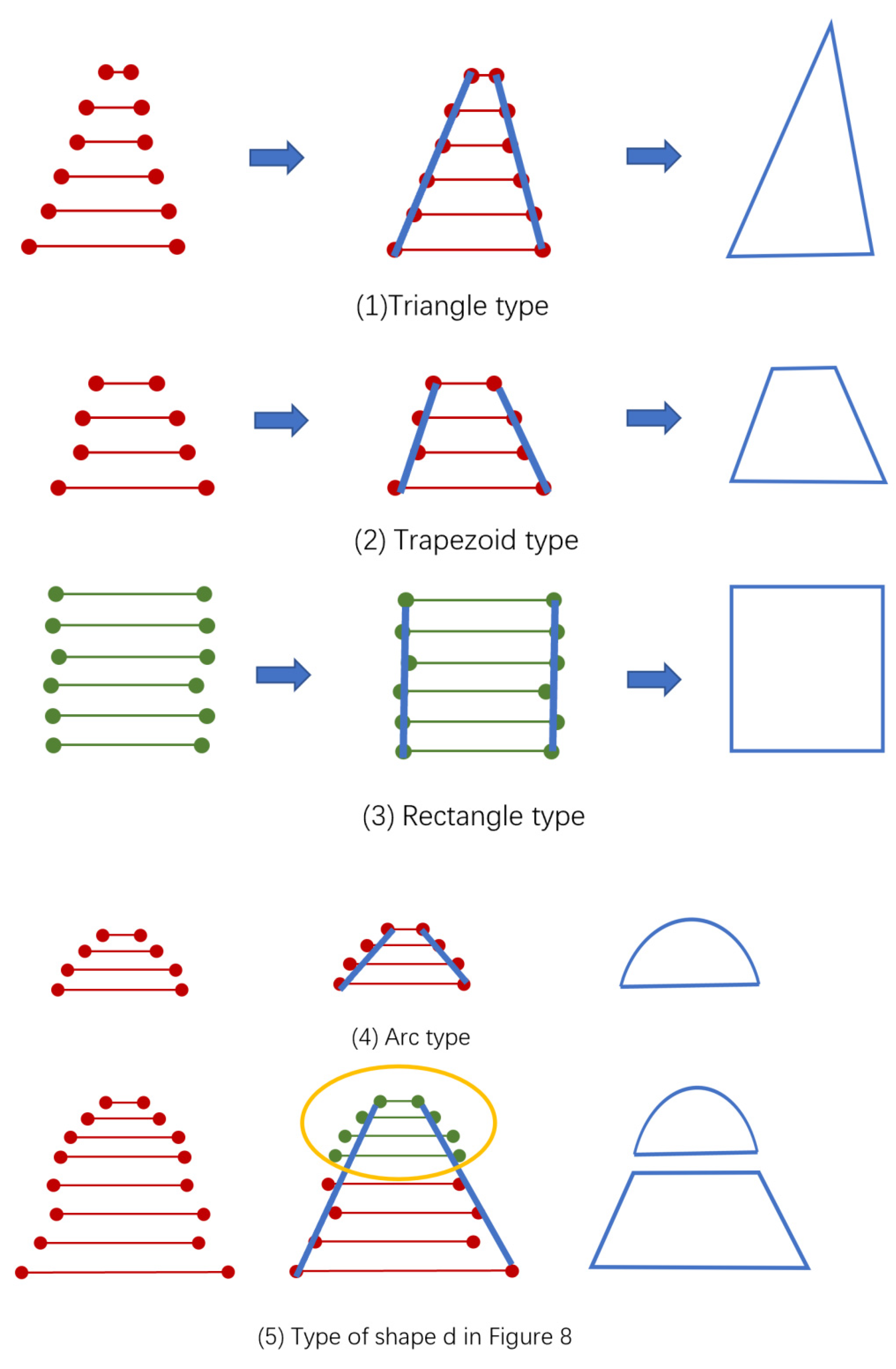
(3) In Figure 10, only a few typical tree geometries are listed. There are more than these tree geometries in the world. With the development of LiDAR technology, the density of point clouds is getting higher, and more details on trees can be obtained. More in-depth methods to use geometric forms need to be further studied and applied.
(4) Each basic geometric feature can be expressed parametrically, taking triangular shape, for example, which has side length and included angle. Therefore, in addition to using the geometric composition for classification, for trees with similar shapes, the value range of different parameters can be used for further classification.
However, the performance of the parallel-line shape fitting method mainly depends on the segmentation results, and Table 5 and Table 6 indicate that the pines, birches, and cedars are easily confused or indistinguishable. There is also a sizable proportion of misclassification in the “other “class. The reasons are summarized as follows:
(1) From the perspective of classified objects, trees with similar geometric shapes are easier to be misclassified, such as pines, birches and cedars in the test site.
(2) The result of classification depends on the result of tree crown segmentation. The result of tree crown segmentation is affected by many factors, e.g., lightning or rocks can cause changes in the geometric shape of trees, and that is the main reason many tree species are wrongly classified into the “other “ class.
(3) If many trees are growing close together, the segmentation results as well as the classification of tree species will be affected. In this survey area, if pines or birches grow together, they are easily identified as cedars, because the segmentation algorithm easily classifies the trees’ points next to each other equally, which makes the triangular shape become a rectangular section structure.
(4) For tree species with single basic geometric structure, such as triangular, rectangular or arc-shaped tree species, the classification accuracy can reach 90%, such as pines, shrubs, etc.
From above, it is clear that in Northeast China, the growth of trees is relatively sparse, the types of tree species are relatively simple, which are mainly coniferous forests and some deciduous forests. Therefore, the method proposed in this paper can obtain better classification results and save manual participation greatly in the forestry survey.
For the complex forest area with complex tree species in the south area, it is difficult to achieve good classification accuracy. Strictly speaking, the geometric shape of trees has the unique characteristics of each tree, and the geometric shape of trees is affected by accidental factors, which often affects the classification accuracy when using the shape fitting method. As a result, in the further work, more shapes or more remote sensing techniques, such as multispectral or radar technology, should be combined with laser radar technology to improve the classification in complex forest areas.

5. Conclusions

In this paper, a rotating profile at a certain angle (RPAA) is used, and the initial segmentation of the crowns is complete; then the accuracy of tree crown segmentation has reached 95%, which provides excellent preparation for tree species classification.
Assuming that the tree crown can be seen as the triangle, rectangle, arc, and other basic shapes, or as combinations of basic geometry, the parallel-line shape fitting method is performed to classify tree species; this type of species classification has an average classification accuracy of 90.9%, and the optimal classification accuracy was 95.9%. It is superior to the parametric crown classification method, which also uses the geometric information of the tree crown, in average accuracy of 87.2% and the highest accuracy of 93.8%; however, the latter often requires full waveform data.
Table 7 shows the accuracy of different tree species classification. Method 1 is an SVM/RF classifier based on fusion data [61]. It works well in general macro-classes, but it is not very suitable for single tree species classification. Method 2 is CNN based on UVA images [49]. It is only applicable to palm classification and does not have universality. Method 3 is the linear discriminant function with a cross validation based on LiDAR intensity data [47]. Its classification rate is higher using leaf-off data (84.3%) than using leaf-on data (73.1%) and is at its highest (90.6%) when combining these two. Method 4 is unsupervised classification based on full waveform LiDAR data [38]. Its results are also different in the data set of leaf-off and leaf-on. Method 5 is DNN based on UAV LiDAR data [62]. It has satisfactory results in the classification of two tree species. Method 6 is the algorithm used in this paper and the method in this paper largely depends on the segmentation results of the tree crown. For trees whose crown geometry is similar to each other or grow too close, the tree species classification usually has poor results, because the original crown shapes are damaged by interwoven crowns. As a result, the method proposed in this paper can obtain better classification results in sparse forest areas. From Table 7, it is clear that the shape fitting method is suitable for tree species classification in sparse areas.
In further work, more shapes should be tested, and the spectral information of the image can be combined, or the phenological information of multi-temporal data can be used to improve the accuracy of tree species classification. But, in the tropical rain forest where tree species grow staggered, tree species extraction and classification are still difficult.

Author Contributions

C.Y. conceived and designed the experiments. C.Q. and J.W. performed the experiments. J.X. analyzed the data. C.Y. and H.M. wrote the paper. All authors have read and agreed to the published version of the manuscript.

Funding

This research was funded by [National Key R&D] grant number [2018YFB0504500], [National Natural Science Foundation of China] grant number [41101417] and [National High Resolution Earth Observations Foundation] grant number [11-H37B02-9001-19/22].

Data Availability Statement

Not applicable.

Acknowledgments

This research is funded and supported by National Key R&D Program of China (2018YFB0504500), National Natural Science Foundation of China (No. 41101417) and National High Resolution Earth Observations Foundation (11-H37B02-9001-19/22).

Conflicts of Interest

The authors declare there is no conflict of interest regarding the publication of this paper. The founding sponsors had no role in the design of the study; in the collection, analyses, or interpretation of data; in the writing of the manuscript; or in the decision to publish the results.

References

  1. Kangas, A.; Gove, J.; Scott, C. Introduction: Forest Inventory; Springer: Dordrecht, The Netherlands, 2006; pp. 3–11. [Google Scholar]
  2. Wulder, M.A.; Bater, C.W.; Coops, N.C.; Hilker, T.; White, J.C. The role of LiDAR in sustainable forest management. For. Chron. 2008, 84, 807–826. [Google Scholar] [CrossRef] [Green Version]
  3. Leckie, D.G.; Gillis, M.D. Forest inventory in Canada with emphasis on map production. For. Chron. 1995, 71, 74–88. [Google Scholar] [CrossRef]
  4. Gillis, M.D.; Omule, A.Y.; Brierley, T. Monitoring Canada's forests: The National Forest Inventory. For. Chron. 2005, 81, 214–221. [Google Scholar] [CrossRef]
  5. Mckinley, D.C.; Ryan, M.G.; Birdsey, R.A.; Giardina, C.P.; Harmon, M.E.; Heath, L.S.; Houghton, R.A.; Jackson, R.B.; Morrison, J.F.; Murray, B.C.; et al. A synthesis of current knowledge on forests and carbon storage in the United States. Ecol. Appl. 2011, 21, 1902–1924. [Google Scholar] [CrossRef] [Green Version]
  6. Roberts, J.; Tesfamichael, S.; Gebreslasie, M.; Aardt, J.; Ahmed, F. Forest structural assessment using remote sensing tech-nologies: An overview of the current state of the art. South. Hemisph. For. J. 2007, 69, 183–203. [Google Scholar] [CrossRef]
  7. Reese, H.; Nilsson, M.; Sandström, P.; Olsson, H. Applications using estimates of forest parameters derived from satellite and forest inventory data. Comput. Electron. Agric. 2002, 37, 37–55. [Google Scholar] [CrossRef] [Green Version]
  8. van Leeuwen, M.; Nieuwenhuis, M. Retrieval of forest structural parameters using LiDAR remote sensing. Eur. J. For. Res. 2010, 129, 749–770. [Google Scholar] [CrossRef]
  9. Culvenor, D.S. TIDA: Analgorithm for the delineation of tree crowns in high spatial resolution remotely sensed imagery. Comput. Geosc. 2002, 28, 33–44. [Google Scholar] [CrossRef]
  10. Turner, W.; Spector, S.; Gardiner, N.; Fladeland, M.; Sterling, E.; Steininger, M. Remote sensing for biodiversity science and conservation. Trends Ecol. Evol. 2003, 18, 306–314. [Google Scholar] [CrossRef]
  11. Smith, B.; Knorr, W.; Widlowski, J.-L.; Pinty, B.; Gobron, N. Combining remote sensing data with process modelling to monitor boreal conifer forest carbon balances. For. Ecol. Manag. 2008, 255, 3985–3994. [Google Scholar] [CrossRef]
  12. Koetz, B.; Sun, G.; Morsdorf, F.; Ranson, K.; Kneubühler, M.; Itten, K.; Allgöwer, B. Fusion of imaging spectrometer and LIDAR data over combined radiative transfer models for forest canopy characterization. Remote Sens. Environ. 2007, 106, 449–459. [Google Scholar] [CrossRef]
  13. Drake, J.B.; Dubayah, R.O.; Clark, D.B.; Knox, R.G.; Blair, J.B.; Hofton, M.A.; Chazdon, R.L.; Weishampel, J.F.; Prince, S. Estimation of tropical forest structural characteristics using large-footprint lidar. Remote Sens. Environ. 2002, 79, 305–319. [Google Scholar] [CrossRef]
  14. Lillesand, T.; Kiefer, R.; Chipman, J. Remote Sensing and Image Interpretation; Wiley: Hoboken, NJ, USA, 2004. [Google Scholar]
  15. Kumar, L.; Schmidt, K.; Dury, S.; Skidmore, A. Imaging Spectrometry and Vegetation Science. In Imaging Spectrometry: Basic Principles and Prospective Applications; Springer: Dordrecht, The Netherlands, 2001; pp. 111–155. [Google Scholar]
  16. Zhen, Z.; Quackenbush, L.J.; Zhang, L. Trends in Automatic Individual Tree Crown Detection and Delineation—Evolution of LiDAR Data. Remote Sens. 2016, 8, 333. [Google Scholar] [CrossRef] [Green Version]
  17. Belgiu, M.; Drăguţ, L. Random forest in remote sensing: A review of applications and future directions. ISPRS J. Photogramm. Remote Sens. 2016, 114, 24–31. [Google Scholar] [CrossRef]
  18. Ballanti, L.; Blesius, L.; Hines, E.; Kruse, B. Tree Species Classification Using Hyperspectral Imagery: A Comparison of Two Classifiers. Remote Sens. 2016, 8, 445. [Google Scholar] [CrossRef] [Green Version]
  19. Ab Majid, I.; Abd Latif, Z.; Adnan, N.A. Tree species classification using worldview-3 data. In Proceedings of the 2016 7th IEEE Control and System Graduate Research Colloquium (ICSGRC), Shah Alam, Malaysia, 8 August 2016. [Google Scholar]
  20. Wong, F.K.K.; Fung, T. Combining EO-1 Hyperion and Envisat ASAR data for mangrove species classification in Mai Po Ramsar Site, Hong Kong. Int. J. Remote Sens. 2014, 35, 7828–7856. [Google Scholar] [CrossRef]
  21. Dostálová, A.; Lang, M.; Ivanovs, J.; Waser, L.T.; Wagner, W. European wide forest classification based on Senti-nel-1 data. Remote Sens. 2021, 13, 337. [Google Scholar] [CrossRef]
  22. Zhao, F.; Sun, R.; Zhong, L.; Meng, R.; Huang, C.; Zeng, X.; Wang, M.; Li, Y.; Wang, Z. Monthly mapping of forest harvesting using dense time series Sentinel-1 SAR imagery and deep learning. Remote Sens. Environ. 2022, 269, 112822. [Google Scholar] [CrossRef]
  23. Lim, K.; Treitz, P.; Wulder, M.; St-Onge, B.; Flood, M. LiDAR remote sensing of forest structure. Prog. Phys. Geogr. Earth Environ. 2003, 27, 88–106. [Google Scholar] [CrossRef] [Green Version]
  24. Bjerreskov, K.S.; Nord-Larsen, T.; Fensholt, R. Classification of nemoral forests with fusion of multi-temporal Sen-tinel-1 and 2 data. Remote Sens. 2021, 13, 950. [Google Scholar] [CrossRef]
  25. NOAA. LIDAR—Light Detection and Ranging—Is a Remote Sensing Method Used to Examine the Surface of the Earth; NOAA: Washington, DC, USA, 2013. [Google Scholar]
  26. Bellakaout, A.; Cherkaoui, M.; Ettarid, M.; Touzani, A. Automatic 3D Extraction of Buildings, Vegetation and Roads from LIDAR Data. In Proceedings of the XXIII ISPRS CONGRESS, COMMISSION III. In Proceedings of the International Archives of the Photogrammetry Remote Sensing and Spatial Information Sciences, Prague, Czech Republic, 12–19 July 2016; Volume 41, pp. 173–180. [Google Scholar]
  27. Ritchie, J.C. Remote sensing applications to hydrology: Airborne laser altimeters. Hydrol. Sci. J. 1996, 41, 625–636. [Google Scholar] [CrossRef] [Green Version]
  28. Mallet, C.; Bretar, F. Full-waveform topographic lidar: State-of-the-art. ISPRS journal of photogrammetry and remote sensing 2009, 64, 1–16. [Google Scholar] [CrossRef]
  29. Holmgren, J.; Persson, Å. Identifying species of individual trees using airborne laser scanner. Remote Sens. Environ. 2004, 90, 415–423. [Google Scholar] [CrossRef]
  30. Popescu, S.C.; Wynne, R.H. Seeing the trees in the forest: Using lidar and multispectral data fusion with local filtering and variable window size for estimating tree height. Photogramm. Eng. Remote Sens. 2004, 70, 589–604. [Google Scholar] [CrossRef] [Green Version]
  31. Chen, Q.; Baldocchi, D.; Gong, P.; Kelly, M. Isolating Individual Trees in a Savanna Woodland Using Small Footprint Lidar Data. Photogramm. Eng. Remote Sens. 2006, 72, 923–932. [Google Scholar] [CrossRef] [Green Version]
  32. Lovell, J.; Jupp, D.; Newnham, G.; Coops, N.; Culvenor, D. Simulation study for finding optimal lidar acquisition parameters for forest height retrieval. For. Ecol. Manag. 2005, 214, 398–412. [Google Scholar] [CrossRef]
  33. Michael, A.L.; Michael, K.; Yong, P.; Plinio, B.; Maria, O.H. Revised method for forest canopy height estimation from Ge-oscience Laser Altimeter System waveforms. J. Appl. Remote Sens. 2007, 1, 013537. [Google Scholar]
  34. Riaño, D.; Meier, E.; Allgöwer, B.; Chuvieco, E.; Ustin, S.L. Modeling airborne laser scanning data for the spatial generation of critical forest parameters in fire behavior modeling. Remote Sens. Environ. 2003, 86, 177–186. [Google Scholar] [CrossRef]
  35. Lee, A.C.; Lucas, R.M. A LiDAR-derived canopy density model for tree stem and crown mapping in Australian forests. Remote Sens. Environ. 2007, 111, 493–518. [Google Scholar] [CrossRef]
  36. Wagner, W.; Hollaus, M.; Briese, C.; Ducic, V. 3D vegetation mapping using small-footprint full-waveform airborne laser scanners. Int. J. Remote Sens. 2008, 29, 1433–1452. [Google Scholar] [CrossRef] [Green Version]
  37. Maltamo, M.; Eerikäinen, K.; Pitkänen, J.; Hyyppä, J.; Vehmas, M. Estimation of timber volume and stem density based on scanning laser altimetry and expected tree size distribution functions. Remote Sens. Environ. 2004, 90, 319–330. [Google Scholar] [CrossRef]
  38. Reitberger, J.; Krzystek, P.; Stilla, U. Analysis of full waveform LiDAR data for the classification of deciduous and coniferous trees. Int. J. Remote Sens. 2008, 29, 1407–1431. [Google Scholar] [CrossRef]
  39. Tong, X.; Li, X.; Xu, X.; Xie, H.; Feng, T.; Sun, T.; Jin, Y.; Liu, X. A Two-Phase Classification of Urban Vegetation Using Airborne LiDAR Data and Aerial Photography. IEEE J. Sel. Top. Appl. Earth Obs. Remote Sens. 2014, 7, 4153–4166. [Google Scholar] [CrossRef]
  40. Selmi, W.; Selmi, S.; Teller, J.; Weber, C.; Riviere, E.; Nowak, D.J. Nowak, Prioritizing the provision of urban ecosystem services in deprived areas, a question of environmental justice. Ambio 2020, 6, 1035–1046. [Google Scholar]
  41. Zięba-Kulawik, K.; Skoczylas, K.; Wężyk, P.; Teller, J.; Mustafa, A.; Omrani, H. Monitoring of urban forests using 3D spatial indices based on LiDAR point clouds and voxel approach. Urban For. Urban Green. 2021, 65, 127324. [Google Scholar] [CrossRef]
  42. Li, X.; Wen, C.; Cao, Q.; Du, Y.; Fang, Y. RETRACTED: A novel semi-supervised method for airborne LiDAR point cloud classification. ISPRS J. Photogramm. Remote Sens. 2021, 180, 117–129. [Google Scholar] [CrossRef]
  43. Liu, M.; Han, Z.; Chen, Y.; Liu, Z.; Han, Y. Tree species classification of LiDAR data based on 3D deep learning. Measurement 2021, 177, 109301. [Google Scholar] [CrossRef]
  44. Bruggisser, M.; Roncat, A.; Schaepman, M.E.; Morsdorf, F. Retrieval of higher order statistical moments from full-waveform LiDAR data for tree species classification. Remote Sens. Environ. 2017, 196, 28–41. [Google Scholar] [CrossRef]
  45. Blomley, R.; Hovi, A.; Weinmann, M.; Hinz, S.; Korpela, I.; Jutzi, B. Tree species classification using within crown localization of waveform LiDAR attributes. ISPRS J. Photogramm. Remote Sens. 2017, 133, 142–156. [Google Scholar] [CrossRef]
  46. Harikumar, A.; Bovolo, F.; Bruzzone, L. An Internal Crown Geometric Model for Conifer Species Classification With High-Density LiDAR Data. IEEE Trans. Geosci. Remote Sens. 2017, 55, 2924–2940. [Google Scholar] [CrossRef]
  47. Kim, S.; McGaughey, R.J.; Andersen, H.E.; Schreuder, G. Tree species differentiation using intensity data derived from leaf-on and leaf-off airborne laser scanner data. Remote Sens. Environ. 2009, 113, 1575–1586. [Google Scholar] [CrossRef]
  48. Qin, H.; Zhou, W.; Yao, Y.; Wang, W. Individual tree segmentation and tree species classification in sub-tropical broadleaf forests using UAV-based LiDAR, hyperspectral, and ultrahigh-resolution RGB data. Remote Sens. Environ. 2022, 280, 113143. [Google Scholar] [CrossRef]
  49. Ferreira, M.P.; de Almeida, D.R.A.; Papa, D.D.A.; Minervino, J.B.S.; Veras, H.F.P.; Formighieri, A.; Santos, C.A.N.; Ferreira, M.A.D.; Figueiredo, E.O.; Ferreira, E.J.L. Individual tree detection and species classification of Amazonian palms using UAV images and deep learning. For. Ecol. Manag. 2020, 475, 118397. [Google Scholar] [CrossRef]
  50. Wagner, F.H.; Sanchez, A.; Tarabalka, Y.; Lotte, R.G.; Ferreira, M.P.; Aidar, M.P.; Gloor, E.; Phillips, O.L.; Aragao, L.E. Using the U-net convolutional network to map forest types and disturbance in the Atlantic rainforest with very high resolution images. Remote Sens. Ecol. Conserv. 2019, 5, 360–375. [Google Scholar] [CrossRef] [Green Version]
  51. Weinstein, B.G.; Marconi, S.; Bohlman, S.; Zare, A.; White, E. Individual Tree-Crown Detection in RGB Imagery Using Semi-Supervised Deep Learning Neural Networks. Remote Sens. 2019, 11, 1309. [Google Scholar] [CrossRef] [Green Version]
  52. Kim, S.; Hinckley, T.; Briggs, D. Classifying individual tree genera using stepwise cluster analysis based on height and intensity metrics derived from airborne laser scanner data. Remote Sens. Environ. 2010, 115, 3329–3342. [Google Scholar] [CrossRef]
  53. Zhao, Q.; Yu, S.; Zhao, F.; Tian, L.; Zhao, Z. Comparison of machine learning algorithms for forest parameter estimations and application for forest quality assessments. For. Ecol. Manag. 2019, 434, 224–234. [Google Scholar] [CrossRef]
  54. Peng, L.; Liu, K.; Cao, J.; Zhu, Y.; Li, F.; Liu, L. Combining GF-2 and RapidEye satellite data for mapping mangrove species using ensemble machine-learning methods. Int. J. Remote Sens. 2019, 41, 813–838. [Google Scholar] [CrossRef]
  55. Wu, C.; Shen, H.; Shen, A.; Deng, J.; Gan, M.; Zhu, J.; Xu, H.; Wang, K. Comparison of machine-learning methods for above-ground biomass estimation based on Landsat imagery. J. Appl. Remote Sens. 2016, 10, 35010. [Google Scholar] [CrossRef]
  56. Pham, T.D.; Yoshino, K.; Le, N.N.; Bui, D.T. Estimating aboveground biomass of a mangrove plantation on the Northern coast of Vietnam using machine learning techniques with an integration of ALOS-2 PALSAR-2 and Sentinel-2A data. Int. J. Remote Sens. 2018, 39, 7761–7788. [Google Scholar] [CrossRef]
  57. Jachowski, N.R.A.; Quak, M.S.Y.; Friess, D.A.; Duangnamon, D.; Webb, E.L.; Ziegler, A.D. Mangrove biomass estimation in southwest Thailand using machine learning. Appl. Geogr. 2013, 45, 311–321. [Google Scholar] [CrossRef]
  58. Tian, Y.; Zhang, Q.; Huang, H.; Huang, Y.; Tao, J.; Zhou, G.; Zhang, Y.; Yang, Y.; Lin, J. Aboveground biomass of typical invasive mangroves and its distribution patterns using UAV-LiDAR data in a subtropical estuary Maoling River estuary, Guangxi, China. Ecol. Indic. 2022, 136, 108694. [Google Scholar] [CrossRef]
  59. Axelsson, P. Processing of laser scanner data—Algorithms and applications. ISPRS J. Photogramm. Remote Sens. 1999, 54, 138–147. [Google Scholar] [CrossRef]
  60. De Berg, M.; Van Kreveld, M.; Overmars, M.; Schwarzkopf, O.C. Computational Geometry; Springer: Dordrecht, The Netherlands, 2000. [Google Scholar]
  61. Dalponte, M.; Bruzzone, L.; Gianelle, D. Tree species classification in the Southern Alps based on the fusion of very high geometrical resolution multispectral/hyperspectral images and LiDAR data. Remote Sens. Environ. 2012, 123, 258–270. [Google Scholar] [CrossRef]
  62. Liu, M.; Han, Z.; Chen, Y.; Liu, Z.; Han, Y. Classification of tree species for three-dimensional depth learning of airborne lidar data. J. Natl. Univ. Def. Technol. 2022, 44, 123–130. (In Chinese) [Google Scholar]
Figure 1. The information of the test site and the ten sample plots. (a) The location of the ten test plots. (b) The plots with green circles are selected for the experiment. (c) 3D overview map of LiDAR points data for the 10 test sample sites.
Remotesensing 15 00406 g001aRemotesensing 15 00406 g001b
Figure 2. Procedure of trees species classification: First, a DEM is generated; second, the normalized tree points are generated; third, rough tree location generation; fourth, a rotating profile analysis algorithm refines the tree locations; fifth, segmentation of the tree crowns; sixth, calculation of the key points from the segmented crowns points; seventh, tree species classification using shape fitting method.
Remotesensing 15 00406 g002
Figure 3. The iteration processing of the ground points generation.
Remotesensing 15 00406 g003
Figure 4. The treetop location. Point 1 and 2 belong to one tree.
Remotesensing 15 00406 g004
Figure 5. The tree locations in the red circles each belong to one tree.
Remotesensing 15 00406 g005
Figure 6. The workflow of original treetop points generation.
Remotesensing 15 00406 g006
Figure 7. The workflow of tree points crown segmentation by a rotating profile analysis algorithm (RPAA).
Remotesensing 15 00406 g007
Figure 8. The subsegment of the profile, and the positions of Pedge and Pcross.
Remotesensing 15 00406 g008
Figure 9. Various tree species with different profile structures.
Remotesensing 15 00406 g009
Figure 10. The profile shapes of the tree crowns. (a) triangle. (b) sector. (c)rectangle. (d) The combination of sector and trapezoid from top to bottom. (e) The combination of sector and triangle from top to bottom. (f) The combination of two triangles from top to bottom. (g) The combination of sector and rectangle from top to bottom. (h) The combination of triangle and rectangle from top to bottom. (i) The combination of sector, rectangle and triangle from top to bottom. (j) The comb-ination of triangle, rectangle and triangle from top to bottom.
Remotesensing 15 00406 g010
Figure 11. The generation of the profile points of the tree crown, X is the direction of the profile.
Remotesensing 15 00406 g011
Figure 12. Using the alpha shapes algorithm to get the shape of the tree crown, and the red spots are the edge points.
Remotesensing 15 00406 g012
Figure 13. The process of the key point generation. The green point defines the key point and the purple one is the unkey point.
Remotesensing 15 00406 g013
Figure 14. The processing of the tree crown shape fitting. (a) The intersection of the parallel line and the line segments of the key points. (b) The trapezoid is finally confirmed from triangle. (c) The sector is finally confirmed from triangle.
Remotesensing 15 00406 g014
Figure 15. The shape fitting of different tree crowns. (1)~(4) shows the fitting process of the basic shape of the crown. Most of the combined shapes are composed of the basic shapes. (5) The fitting process of shape D in Figure 10 is particularly evident.
Remotesensing 15 00406 g015
Figure 16. The rough tree number and calculated tree number in each plot with different values of parameters d and HT. The blue curve represents rough tree numbers of each plot, the green dashed line represents the final calculated tree number obtained from the RPAA and the orange curve represents the true tree numbers measured on the sample plots.(a) The segmented tree number when d = 1 m and HT = 1 m.(b) The segmented tree number when d = 2 m and HT = 1 m. (c) The segmented tree number when d = 2 m and HT = 1 m. (d) The segmented tree number when d = 2.5 m and HT = 1 m. (e) The segmented tree number when d = 1 m and HT = 1.5 m. (f) The segmented tree number when d = 1 m and HT = 2.0 m. (g) The segmented tree number when d = 1 m and HT = 2.5 m.
Remotesensing 15 00406 g016
Figure 17. Single tree segmentation results of ten plots.
Remotesensing 15 00406 g017
Figure 18. The definition of the R t r i a n g l e .
Remotesensing 15 00406 g018
Figure 19. The tree species classification results of the 10 plots.
Remotesensing 15 00406 g019
Table 1. The details of the test data in Hupao National Park.
Properties of the DataContents
Attitude of points (m)1000
Points density (pts/m2)20
LiDAR scanner typeriegl-vq-1560i
Overlap of flight lines20%
Horizontal accuracy(cm)15~25
Vertical accuracy15
Flight platformCessna 208b aircraft
Table 2. Tree species information for ten plots.
Tree SpeciesNumberPlot ID
Pine233Plot 1~Plot 10
Birch109Plot 2, Plot 5
Cedar113Plot 3, Plot 4, Plot 7
Tsubaki67Plot 2, Plot 7, Plot 9, Plot 10
Shrub148Plot 3, Plot 6, Plot 8, Plot 9
Others111Plot 1~Plot 10
Total781Plot 1~Plot 10
Table 3. The rough tree number and calculated tree number in each plot with different values of parameters d and HT.
Plot IDd = 1, HT = 1d = 1.5, HT = 1d = 2, HT = 1d = 2.5, HT = 1d = 1, HT = 1.5d = 1, HT = 2d = 1, HT = 2.5TTN
RTNCTNRTNCTNRTNCTNRTNCTNRTNCTNRTNCTNRTNCTN
135712516712111010973109307121224121187106118
2168969792919191911429611596838190
3151587351454545451235410754674550
415384817568684646117778971696374
5454342423939272744433735312942
613171716767674141114686761433766
713268666566654545121667957484165
824912112511910710771711791181291099792116
9165678359545438381256110353594958
1020511011710597976565165105133937976102
Note: RTN: Rough Tree Number, CTN: Calculated Tree Number, TTN: True Tree Number.
Table 4. The shape and parameters of the tree samples.
Tree Species IDSample NumberBasic Shape TypeParameter TypeParameter Range
01-Pine20Triangle R t r i a n g l e (2.1, 4.7)
02-Birch10arc and trapezoid————
03-Cedar10arc and rectangle————
04-Tsubaki8Triangle R t r i a n g l e (0.8, 1.4)
05-Shrub15Arc————
Table 5. The classification result comparation of the parallel-line shape fitting method and LiDAR Metrics.
Tree IDCorrect ClassifiedType I ErrorType II ErrorCorrect Rate
Shape FittingLiDAR Metrics
01-Pine217231693.1%92.5%
02-Birch98131189.9%88.3%
03-Cedar9571884.1%87.1%
04-Tsubaki638494%86.3%
05-Shrub1425695.9%93.8%
06-Others98121388.3%75%
Average___90.9%87.2%
Table 6. The details of the tree species misclassification.
01-Pine02-Birch03-Cedar04-Tsubaki05-Shrub06-OthersOA (%)Kappa
01-Pine21761222193.140.8935
02-Birch698300289.91
03-Cedar529500084.08
04-Tsubaki200632494.03
05-Shrub0000142595.95
06-Others333229889.1
Table 7. The accuracy of different tree species classification method.
NO.AccuracyMethodDataSpeciesStudy Area
176.5%SVM/RFFusion data7 species and a “non-forest” classa mountain area in the Southern Alps
298.6%CNNUVA images3 palm species135 ha within an old-growth Amazon forest
390.6%linear discriminant function with a cross validationLiDAR intensity data8 broadleaved and 7 coniferous speciesthe Washington Park Arboretum, Seattle, Washington, USA
496%(leaf-off)
85%(leaf-on)
Unsupervised classificationFull waveform LiDAR dataConiferous, deciduousin the Bavarian Forest National Park
586.7%DNNUAV LiDAR dataBirch and larchSaihanba National Forest Park
690.9%Shape fittingLiDAR data6 speciesthe Hupao National Park
Disclaimer/Publisher’s Note: The statements, opinions and data contained in all publications are solely those of the individual author(s) and contributor(s) and not of MDPI and/or the editor(s). MDPI and/or the editor(s) disclaim responsibility for any injury to people or property resulting from any ideas, methods, instructions or products referred to in the content.

