

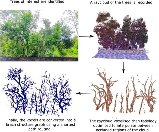
Tree Reconstruction Using Topology Optimisation

Robotics and Autonomus Systems Group, CSIRO Data61, Pullenvale, QLD 4069, Australia
*
Author to whom correspondence should be addressed.
†
These authors contributed equally to this work.
Remote Sens. 2023, 15(1), 172; https://doi.org/10.3390/rs15010172
Submission received: 17 October 2022
/
Revised: 15 December 2022
/
Accepted: 22 December 2022
/
Published: 28 December 2022
/
Corrected: 25 May 2023
(This article belongs to the Special Issue 3D Point Clouds in Forest Remote Sensing II)
Abstract
:Generating accurate digital tree models from scanned environments is invaluable for forestry, agriculture, and other outdoor industries in tasks such as identifying fall hazards, estimating trees’ biomass and calculating traversability. Existing methods for tree reconstruction rely on sparse feature identification to segment a forest into individual trees and generate a branch structure graph, limiting their application to easily separable trees and uniform forests. However, the natural world is a messy place in which trees present with significant heterogeneity and are frequently encroached upon by the surrounding environment. We present a general method for extracting the branch structure of trees from point cloud data, which estimates the structure of trees by adapting the methods of structural topology optimisation to find the optimal material distribution to interpolate the input data. We present the results of this optimisation over a wide variety of scans, and discuss the benefits and drawbacks of this novel approach to tree structure reconstruction. Our method generates detailed and accurate tree structures, with a mean Surface Error (SE) of 15 cm over 13 diverse tree datasets.
1. Introduction
Automatically converting a 3D point cloud of a natural scene into a geometric description of its trees is important in both digital and outdoor industries. It is valuable in forestry to measure biomass and growth of a managed forest, it is needed by power companies to identify branches encroaching on power lines, and it is valuable in bush fire management and post-fire fall risk assessments. In general, it is important in any form of digital twinning, for an accurate digital clone of vegetated environments.
Digital tree reconstruction is challenging because vegetated environments are extremely varied. For example, trees may be tall pines or wide figs, they may be foliated or bare, overlapping or separated, topiarised or unmanaged. The trunks may be obscured by vegetation, and the ground could be sloped or vegetated. In addition to the variety of vegetation, the acquisition can also be varied. 3D point clouds can be collected from ground or aerial lidar, depth cameras or reconstructed from sets of 2D images. Depending on the sensing mode and collection method, the density of points in the point cloud, viewing angle and accuracy can vary significantly. Lastly, dense vegetation often obscures or occludes the scene behind it, resulting in missing branches, trunks and low point density in obscured regions. At its most severe, it may be only the outer canopy that is observed, and for aerial data it may be only the upper canopy with no visible trunks.
This variability makes the task difficult for traditional tree reconstruction methods, which rely on uniquely and accurately identifying common features of trees, such as crowns, trunks, and cylindrical branches. These features are often poorly distinguished or obscured. As a result, robust tree reconstruction in general environments remains elusive, and so leading methods provide tree reconstruction solutions for only special-case environments. Whether that be specialising to conifer forests [1], to high resolution data [2], or to tree environments with clearly resolved trunks [3].
We investigate tackling the tree reconstruction problem from the perspective of topology optimisation, in particular using topology optimisation as a dense reconstruction method. The proposed method acts on all sensor observations equally to interpolate the lidar points with contiguous acyclic tree structures that avoid all observed free space. Rather than searching for sparse features such as crowns, trunks or cylindrical branches, it finds an efficient distribution of material (wood) that matches the input data under a small number of assumptions. These are:
- the input data represent ground, low lying vegetation and trees only
- trees are solid acyclic structures that connect to the ground, with no gaps
- unobserved trees have a similar branching angle
- unobserved structures use their material ‘efficiently’, having approximately straight branches
The meaning of ‘efficiently’ here depends on the choice of cost function. We employ a minimal and standard topology optimisation cost function: compliance under linear scalar loads. This is described in Section 3.1 and Section 3.2.
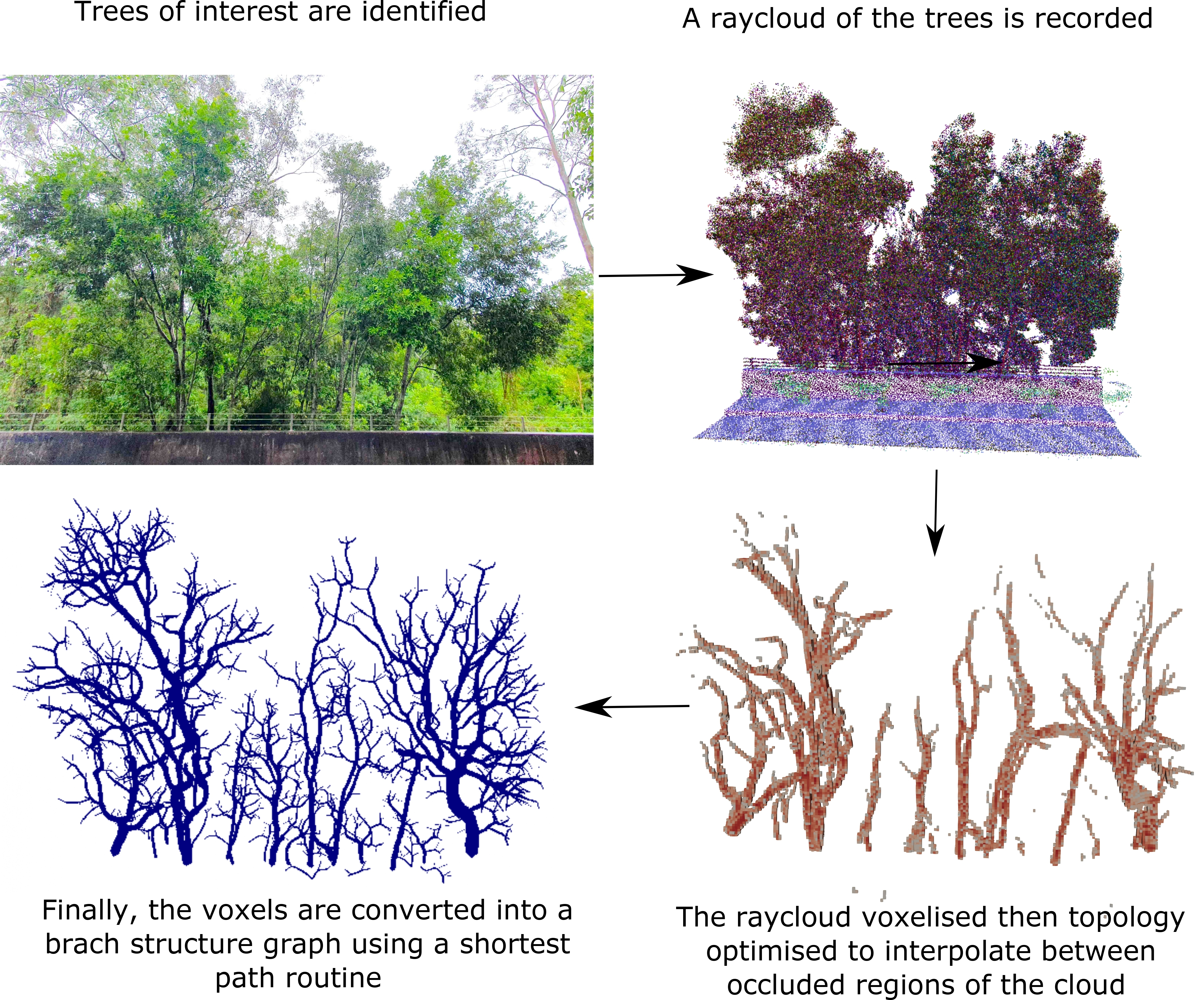
We believe that this approach makes fewer assumptions about the nature of the data than traditional reconstruction approaches, and that its failures are likely to be less extreme, giving results that are tree-like and connected even where significant trunk and branch data are missing. Reducing the severity of any failures is important because bulk measures such as number of trees, number of branches and biomass, can remain reasonable. This robustness is shown in Figure 1, in which a set of trees (blue) are extracted from a 3D point cloud (green) using our method. Despite several intertwined trees and a barrier occluding the tree-trunks, the tree branches closely match the measured point cloud and it plausibly estimates unobserved regions. We validate this claim in Section 6.1 and Section 6.2.
To clarify the tree reconstruction problem, we first specify the input and output data structures that we will use. The input data can come from a number of sensors, most commonly lidar (mobile or static, ground based or aerial), but also depth cameras and binocular cameras. For brevity, we will refer to the input sensor as a lidar in this paper as it is the most commonly used solution for these environments. The lidar data are then processed with a registration scheme (such as Simultaneous Localisation and Mapping, SLAM) to transform the observations into a common coordinate frame. The result is a set of 3D points and a set of rays from each sensor location to the observed 3D point. The set of 3D points represents physical surfaces and the set of rays represents free space. The data may also contain rays that have no end point, such as those pointing towards the sky.
If the set of rays is not provided directly from the registration scheme, then it can be generated from the set of 3D points and the calculated trajectory of the sensor, provided that they both contain time stamps in order to find the corresponding ray start and end locations. For static lidars, there may be no explicit trajectory provided, but the origin of each scan is typically available, so the set of rays can also be constructed in this case.
The set of all of these rays and points represents the principle input data that have been observed from the scene, and is referred to as a ray cloud, as opposed to a point cloud, which is only the set of points.
The output data are a piecewise-cylindrical acyclic graph, representing the surface geometry of the trees in the scene. This Branch Structure Graph (BSG) is the set of nodes defined by: a 3D node location, a reference to the parent node, and a radius for the cylinder between the node location and the parent node’s location. The root node of each tree contains no parent. Unlike in [4] we allow the graph to be disconnected, so a single graph represents the set of trees, and so the output of our method is a single BSG.
The problem that we address in this paper is how to robustly transform a ray cloud of a natural scene into a BSG representation of its trees. To the best of the authors’ knowledge, this paper presents the first time use of topology optimisation as a method for physics-informed geometric reconstruction. Our main contributions are:
- the development and investigation of a novel tree reconstruction method based on topology optimisation, which allocates biomass to minimise a specified cost function
- the development of a branch structure generation algorithm, which converts the optimised voxel trees into a graph of their branch structures
- its application to a dataset of realistic natural scenes chosen to assess common failure cases systematically
2. Existing Work
2.1. Tree Reconstruction
The most common approach to tree structure reconstruction from point clouds is a two stage approach. The first stage segments the data into individual trees, and the second stage extracts the branches of a single-tree point cloud.
The segmentation phase has many variants, which reflect the variety of features that may be used to separate trees. Trunk identification methods [5,6,7,8] look for near-vertical cylindrical shapes in the point cloud as the basis for locating the individual trees. Crown methods [9] look for conical or dome-shaped crowns within the point cloud. More recently, gap-based methods [10,11] use spectral clustering or agglomerative clustering [12] to separate trees based on any gap or thinning of foliage between adjacent trees. Lastly, branch direction methods [13] look at average branch directions in order to estimate a central trunk location, and assign trunk ownership to each branch in a forest point cloud.
These methods are effective in special cases, such as managed pine forests, or sparse woodland. However, in general point clouds, each feature has many failure cases: trunks are typically unobserved from aerial data, crowns are poorly observed from ground-based scanning, and gap-based methods lose reliability on densely overlapping trees. Lastly, branch direction methods fail on highly foliated trees, where the branches are occluded by leaves. Deep learning-based methods have recently emerged that are able to semantically segment point clouds with high accuracy in woody forests [14]. However these require large amounts of labelled training data to perform well, and have not been shown to generalise to more complex and diverse environments.
There are branch reconstruction methods available that construct the tree skeleton using medial axis methods [15,16], thinning [17], region growing [18] and cylinder slices [2], see [19] for a comparative review. The most prominent of these is the distance segmentation method [15,20] first described in 2007 [21]. This method finds the shortest path tree from root to all cloud points, and groups each point by path distance from root. The result is a set of approximately cylindrical sections, which can be converted into the tree structure (BSG) nodes. This general approach is available in the software treeQSM [22], AdTree [3], and AdQSM [23] which is based on AdTree. These methods require well-sampled branches in order for the shortest path algorithm to connect the points appropriately, and a well-defined trunk in order to ascertain the root position of the path. Moreover, these and the other cited branch reconstruction algorithms require the point cloud of a single tree. They therefore depend on tree segmentation and so inherit the discussed failure cases of the existing segmentation methods.
2.2. Topology Optimisation
Topology optimisation (TO) is a computational design method which finds the material distribution that minimises a specified cost function. Typically it is used to generate stiff, lightweight structures, such as bridges and mounting brackets. However, it has been applied to a vast range of problems across numerous physical domains, including thermal conductivity problems (heat sinks) [24], compliant mechanisms [25,26,27], soft robots [28,29], electrothermal actuators [30], fluidic actuators [31], fluidic mixers [32], and biomimetic design [33]. Regardless of application, the design space is parameterised by a set of elements, loads, and boundary conditions which enables their governing physical equations to be evaluated using a finite element solver. Iteratively evaluating a candidate design and updating it with a gradient-based or heuristic non-gradient solver then allows a high-performing design to be identified. For a detailed review of topology optimisation methods and applications see [34,35,36,37,38].
Compared to the previously discussed methods, topology optimisation offers a generalised, dense approach to tree structure reconstruction, rather than the sparse identification of features of previous methods.
In this work, we use TO as an inverse design tool, to reconstruct a tree given an incomplete set of measurements. That is, it estimates the branch geometry wherever it is not directly observed. To our knowledge, TO has not previously been employed as an inverse design tool, and has not previously been used for tree reconstruction from point clouds.
In this paper, we use the open source software PANSFEM2 [39] as the basis for the topology optimisation solver (Section 3.1). The software does not have an accompanying paper, but its topology optimisation method is very similar to Andreassen et al [40], including the Heaviside projection filter option.
3. Method
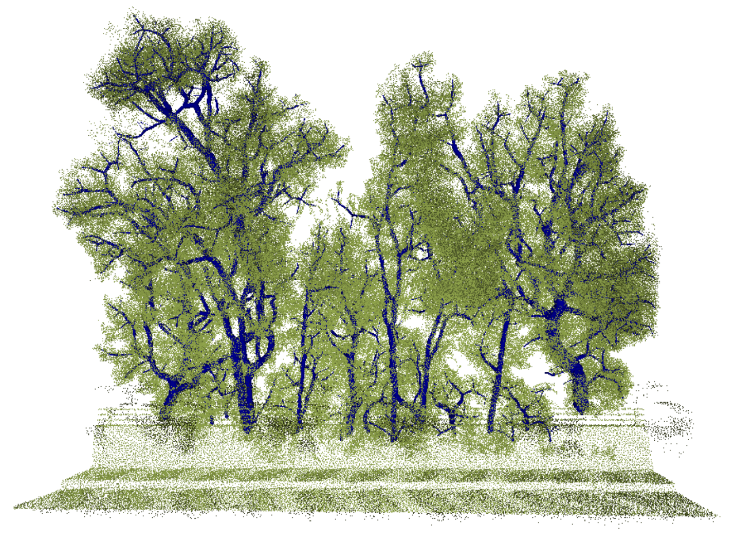
Our approach to tree reconstruction from lidar data is to interpolate the lidar samples and the ground with an efficient distribution of woody material. This optimal material distribution problem is what is solved using topology optimisation. We now describe this standard topology optimisation formulation, followed by our set of adaptations for application to tree reconstruction in Section 3.2, Section 3.3, Section 3.4, Section 3.5 and Section 3.6. The main stages of this process are depicted in Figure 2.
3.1. SIMP Topology Optimisation
The standard approach to topology optimisation is based on iteratively solving a structural problem using the finite element method (FEM). The design space is discretised into a 3D grid of cubic elements (voxels) and the grid nodes (vertices). The stiffness of each element index i is taken as a function of the ‘pseudodensity’ design parameter using the Solid Isotropic Material with Penalization (SIMP) method:
giving physical values of between solid , and void which is small but non-zero to avoid singularities. The penalty exponent p drives convergence to a binary final solution, where .
The optimal design is formed as a constrained minimisation of the system’s total compliance :
where the total volume of woody material has a prescribed upper limit , and N is the total number of voxels.
The global displacement matrix is composed of per-element vectors , which are in turn composed of eight nodal displacements . Likewise, the global load matrix is composed of per-element load vectors that are composed of eight nodal loads . The global stiffness matrix is composed of per-element stiffness matrices .
To avoid ‘checkerboard’ distributions of pseudodensity, a spatial filtering and projection scheme is implemented, similar to [41,42]. First it smooths the elemental density accord to the average density of elements in the surrounding neighbourhood:
where is the set of elements within distance voxel widths of i, is the filter weighting between elements i and j, given by , and is the Euclidean distance between elements i and j. The smoothed density is then ‘projected’ through a smooth approximation of the Heaviside step function to obtain a more binary pseudodensity according to:
where is the filter steepness parameter.
Equation (2) is solved using the CONLIN solver [43], which solves a sequence of linearised subproblems and uses the sensitivities (Jacobian) of the system to increase solver efficiency. The sensitivities of the cost with respect to the densities can be found in Appendix A.
3.2. Application to Tree Reconstruction
The topology optimisation is subject to two boundary conditions. The Dirichlet condition sets the displacements to zero on the nodes closest to the ground, as estimated in Section 3.4. The Neumann boundary condition fixes the nodal load in proportion to the number of lidar points that are closest to this node. The solved pseudodensity distribution then represents the distribution of wood in the scene, which is the set of branches.
The resulting voxel tree is therefore the structure connected to the ground that is most efficient at resisting the loads applied at the lidar points. Unlike typical structural optimisation, we do not use vector loads and displacements, representing gravitational force and sag, instead we use scalar loads and displacements. This is a non-directional representation that is mathematically equivalent to the thermal model of topology optimisation, only using structural terms (load, displacement, stiffness) rather than the thermal equivalents (heat, temperature and thermal conductivity).
This scalar model guarantees that the resulting structures are topologically trees (acyclic graphs), unlike the (cyclic graph) truss structures that are a signature of gravitational structural optimisation. The structures are also always contiguous and connected to the ground (the Dirichlet boundary), and the requirement to minimise compliance preferences straight branches between lidar points. This is because the compliance at the end of a curved branch is integrated over a greater length than that of a straight branch, and the compliance is being minimised. All of these properties fit with our assumptions about the input data that we listed in Section 1.
Because this method is not identifying sparse features, the problem does not become underdetermined when such features are missing. This is because the state equation ensures that there is an underlying physical model (a prior) wherever data are missing. For this reason, tree structures occur even when there only 5 points in the cloud and no ray information (see Figure 3), or even if the cloud were a set of randomly sampled points, or contained walls or cyclic structures like pylons. In every case this scalar model of topology optimisation will generate the lowest compliance acyclic structures to connect the available data to the ground.
3.3. Controlling Branch Angle
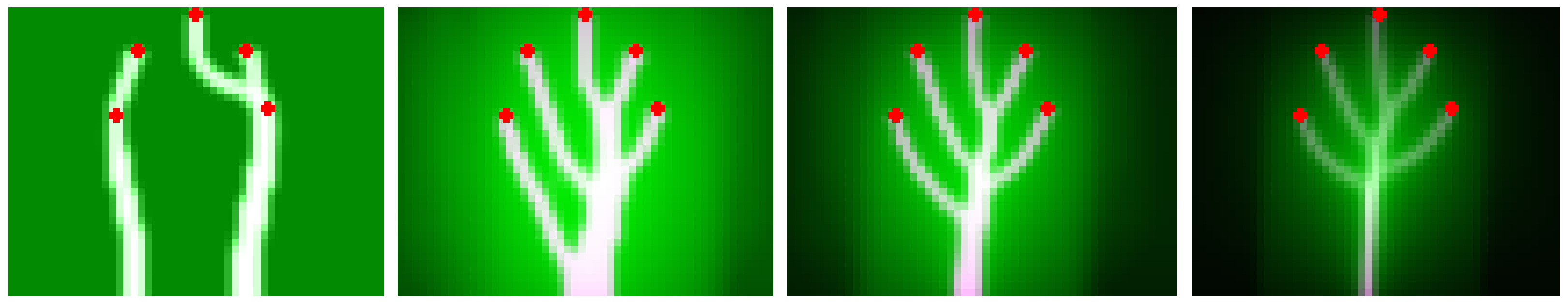
The above system generates a tree structure of woody material to match the specified point sources. The closer this tree structure is to the shape of real trees, the more accurate its interpolation will be in unobserved regions. Unfortunately the generated tree structure has a fairly narrow branch angle and it has been demonstrated [44] that this angle reduces to zero in the highest fidelity solutions. It is therefore important to be able to preference larger branch angles, in particular to control this angle through a parameter, according to the type of trees in the scene.
We do this by including an additional spatial low pass filtering kernel, applied for each element i:
where is the distance in voxels between i and j in the 3D grid. This is used as a multiplier on the stiffness:
for some , where represents the standard solution and produces larger branch angles in unobserved regions.
Excluding discretisation artefacts is proportional to branch cross-sectional area for any particular branch shape. So Equation (6) scales stiffness as a power of the branch’s thickness. Due to the higher stiffness of the thicker branches, the smaller ones can connect to them farther from the sink, which makes the branching angle larger, as seen in Figure 3.
3.4. Estimating Ground
We estimate the ground surface height from the ray cloud by interpolating the set of ‘lowest points’. We define these lowest points as each point with gradient to every other point less than some gradient g. Specifically the set of point indices . This can be thought of as a sand model of the terrain height, since dry sand settles up to a maximum gradient. The interpolation is achieved by removing the z component of the set of lowest points, calculating its Delauney triangulation, then restoring the z component to the triangle vertices. This triangular mesh allows a ground height to be calculated for any horizontal location within the Delauney triangulation. We use the open source library raycloudtools [45] for a fast implementation of this ground surface reconstruction.
3.5. Free Space
In addition to lidar points, the lidar rays themselves serve an important role in mapping out the free space (the air) in the scene. This is important in preventing the algorithm from generating branches in regions that are observed to be free space. The free space is mapped by using quarter-width subvoxels to record the presence of any ray that passes through the subvoxel. This is achieved by ‘walking’ each ray through the subvoxel grid using a line drawing algorithm, if any ray passes through a subvoxel then it is flagged as unoccupied. The 64 unoccupied statuses can be encoded in a single long integer per voxel, and the number of occopied subvoxels divided by 64 provides the maximum density value for each voxel i.
3.6. Branch Structure Graph
The output of the optimisation process is a grid of voxels containing density values from zero to one. These densities form a treelike structure, with voxel density representing the percentage of coverage of the underlying tree. This is a useful data structure in its own right, and can be used for physical simulation, biomass estimation and other metrics, but it is also valuable to convert the results into the Branch Structure Graph (BSG) referred to in Section 1. This provides a canonical description of the topology and geometry of the trees.
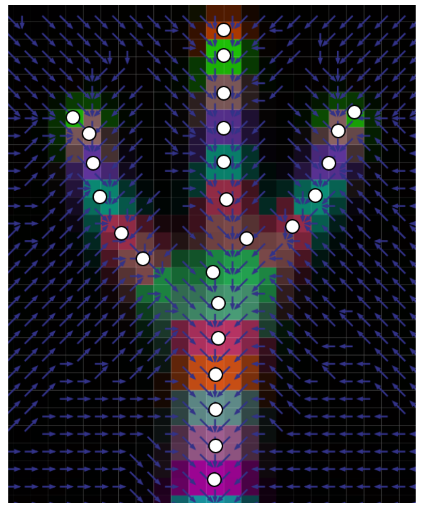
In order to extract the graph, we employ a variation of the distance bucketing method used on point clouds [20,21,46]. Our method uses Dijkstra’s algorithm [47] to generate the shortest path forest between the lowest non-empty voxels and all other non-empty voxels, considering the nearest 26 voxels (the Moore neighbourhood) for each voxel. Rather than use Euclidean distance between voxel centres, we divide the Euclidean distance to each neighbour by its density value. This rewards paths that follow the densest set of voxels. We then use the Euclidean path distance from the ground to bucket the voxels into distance intervals that are two voxels wide.
For each bucket, all voxels less than a density threshold are removed and the bucket is split into one tree segment for each connected set of voxels S. Each tree segment’s parent is recorded, then its centroid and radius are calculated according to:
where is the centre of voxel i, and w is the voxel width. The density threshold is set at one quarter of the maximum density value of the parent segment. This threshold therefore reduces on the thinner branches, ensuring that these low density structures are also represented.
This process of splitting the buckets into segments and connecting to the parent segment is repeated until a full graph of centroids and radii is formed, which is the BSG. Figure 4 illustrates this process on a two-dimensional tree, with one colour per bucket and the resulting BSG centroids shown as white disks. The branches below a certain radius can be cropped to avoid reconstructing branches that are too small compared to the voxels that they are representing. We crop branches when in our experiments.
4. Experiments
We assess our method using 21 acquired datasets from our research site in Pullenvale, Australia. These were acquired using scanners based on a rotating Velodyne VLP16 lidar, and registered into a 3D point cloud using the Wildcat SLAM software [48]. The datasets cover a wide range of vegetated environments, including multiple tree species such as figs, eucalypts, palms and a monkey puzzle tree; and a wide range of heights from 1.5 m up to 28 m. They have been captured specifically to assess our method under the typical failure cases of existing tree segmentation and reconstruction algorithms, and are labelled as (failure) case #1 to #21.
The aim of this data is to test our hypothesis that the topology optimisation approach has fewer or less extreme failure cases than the existing methods that rely on sparse features. The experiments are therefore a study of the ability to generate trees that fit to poorly-defined and varied input data. We consider this to be an assessment of the robustness of the algorithm to these varied environments. Here we explain the choice of failure cases:
- Non-problematic:
- these are included for completeness and are cases #1 and #2
- Disconnected canopies:
- these are sections of canopy that do not connect to the ground due to cropping the scan, or due to the tree being only partially observed. They are included in cases #3 and #4 as they are a common boundary issue that affects all reconstruction methods.
- Hidden trunks:
- Non-tree objects:
- the majority of reconstruction algorithms assume that there are no non-tree objects in the scan, we have therefore included scans with a shelter (#5), walls (#9, #18) and lamp posts (#7, #14 and #17)
- Canopy close to ground:
- Overlapping trees:
- V-shaped trunk:
- Hidden branches:
- most branch reconstruction methods and some segmentation methods [13] rely on clearly observable branches so we include scenes with hidden branches in cases #14 to #21
- Ambiguous crowns:
- for those that rely on crown features [9] we include poorly identifiable crown scans in cases #11 and #15. Trees tucked under other trees are a failure case for crown extraction algorithms that consider only the upper canopy, so we include this situation in case #18
- Uneven ground:
- sloped and uneven ground needs to be considered in natural environments, this is represented in case #19
- One-sided scan:
- this is included in order to observe biases in tree structures due to the scan being acquired from principally one direction, and occurs in cases #9 and #21
In cases #2 to #4, we removed reflections off the ground, which cause erroneous underground points that disturb the ground surface estimation. There was no other pre-processing of the 3D ray clouds.
Ground height was estimated using the described method with gradient everywhere, but to cater for the single steep gradient case #19. All points less than 30 cm above the ground were excluded from applying a load. This is to avoid the algorithm generating branches along the ground, and to reduce the presence of undergrowth in the final result. All scans are processed with the same design parameters: , and wood volume where is the volume of voxels containing lidar points. We run for 20 iterations, over which we ramp up the parameters p from 1 to 3, and from 1 to 4, as a form of annealing to discourage early local minima.
The experimental results for all of the scenes that we scanned are presented in Table 1, Table 2, Table 3, Table 4, Table 5 and Table 6 and Figure 5, and they represent in order: a qualitative study, a quantitative comparison, an ablation study, an aerial comparison, an occlusion study and a voxel size sensitivity study.
The qualitative study (Table 1 and Table 2) visually compares the output BSG to the input scan. The left image is the set of ray cloud end points (the point cloud). The next column image is a rendering of all voxel pseudodensities , which indicates the main wood regions in the raw solver output, but excludes the thinnest branches where . Any differences between this and the wood structure in the point cloud image represent inaccuracies in the topology optimisation part of the algorithm (Section 3.1, Section 3.2, Section 3.3, Section 3.4, and Section 3.5). The next column shows the BSG output, rendered as blue cylinders, this rendering does show the thinner branches. Any other differences between this and the voxelised result represent inaccuracies in the BSG reconstruction (Section 3.6). The exposed branches and trunks in the left image can be compared directly to the BSG branches, and we encourage the reader to view this paper’s accompanying data for further comparison.
In order to compare against existing reconstruction methods, we recall that available methods rely on a two-stage approach of tree segmentation followed by single-tree reconstruction. We test against just the first stage with the understanding that poor tree segmentations will necessarily generate poor branch reconstructions, due to the single-tree requirement of the second stage. In the right hand column we compare to the tree segmentation in the TreeSeparation method [12,49], each colour represents a separate identified tree, so a correct segmentation would show a unique colour for each tree in the ray cloud.
The quantitative comparison (Table 3) quantifies the accuracy of these 13 cases, and compares them against two other existing methods. The accuracy measurement is described in Section 5. We assess the tree segmentation accuracy on two established methods Treeseg [8,50] and TreeSeparation [12,49], and compare that to the number of principle trees that our method reconstructs. We calculate this as the number of trees with trunk diameter more than 30% of the maximum trunk diameter to avoid counting small pieces of undergrowth. Lastly, we have manually inspected the point clouds and counted the number of principle trunks visible in these clouds, using the same criterion.
Both segmentation libraries require a pair of parameters to be set, reflecting the average scale of the trees in the datasets. In both cases, the parameters were within expected ranges and performed better than the default values. For Treeseg, the minimum and maximum stem diameters were set to 0.05 m and 1 m respectively. For TreeSeparation, the voxel height was set to 1.5 m, while the minimum tree diameter was set to 5 m for the widely spaced cases (#1 to #5) and 3 m for the remaining denser cases.
The ablation study (Table 4) compares the reconstruction results for two different values of the convolution kernel parameter . This parameter is only significant when whole branches are occluded. So we assess the performance for two values of this parameter ( and ) for the six most occluded cases. The results match the behaviour in Figure 3.
In the aerial comparison (Table 5), we compare a dense handheld scan to a sparse sparse aerial scan of the same Morton bay fig tree. This aerial scan does not observe the trunk at all, and neither scan has identifiable observations of the tree’s internal branches, due to its thick foliage.
An occlusion study (Table 6) assesses our algorithm’s robustness to occluded branches inside a tree’s canopy. For this, we have taken a tree with visible branches (case #5) and have manually removed the features that do not fit the assumptions of the algorithm, such as the shelter and a lamp post, so that they are not part of the accuracy assessment. We have then generated an occluded version of this ray cloud, removing all points and ray sections within a radius of each tree centre. Lastly, we calculate the accuracy of the reconstructed BSG of this occluded ray cloud against the original unoccluded ray cloud. This is performed for multiple different radius values. We have chosen to employ this spherical occlusion because it is simple and reproducible, and because it represents a worst-case form of occlusion where central observations are completely absent. The reconstruction accuracy measure is described in the following section.
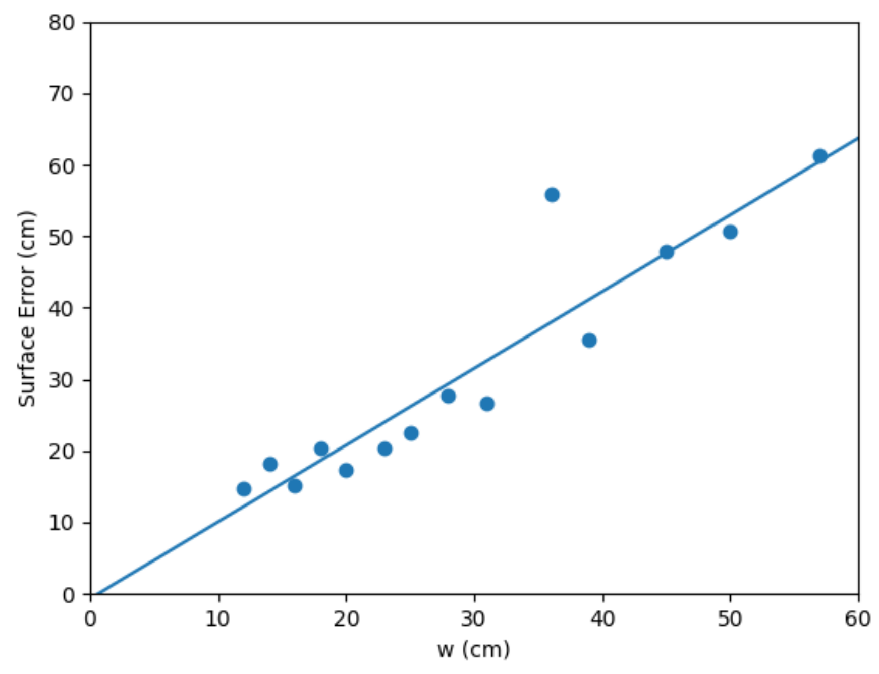
Finally, the sensitivity study (Figure 5 ) evaluates the reconstruction accuracy for different choices of voxel size w. It uses the same dataset as the occlusion study (case #5 with artificial objects removed), and assesses the Surface Error for voxel counts of 6 million and 4 million voxels, and descending powers of two for each. The cubic voxel grid width w (rounded to the nearest centimetre) that best fits these counts is then used for each sample. It results in slightly altered voxel counts from 6.69 million down to 66,096 voxels, approximately a 100-fold range.
5. Accuracy
In order to measure how well the tree reconstruction fits the input point data, we begin by manually removing points that are not part of the reconstructed trees. This includes ground points, undergrowth, fences, points from the moving user, and tree canopy from trunks outside of the bounding box. Whilst this process is performed manually, the features are distinct and relatively unambigious.
The measure that we then use represents the average surface error of the reconstructed tree branches relative to the set of remaining points P. We will refer to it as Surface Error or SE, it is calculated by finding the set of points closest to each cylindrical branch segment i:
where is the unsigned distance between point p and the surface of cylinder , and n is the number of cylinders in the BSG. The mean distance error for cylinder i is therefore:
We then take the surface-area weighted average of the mean distance errors:
where is the surface area of cylinder i (excluding end disks).
We set the weight to the cylinder surface area because the BSG is a surface representation of the observed surface points of the branches, so the surface is the object that we are measuring the accuracy of. It is possible to set the weight to the cylinder’s length or its volume, which roughly correspond to the accuracy of the tree skeletons and their volumes respectively.
Setting the weight to would give the mean distance between points and the reconstructed surface, as has been used previously in assessing tree branch reconstruction [3]. Unlike this choice, SE is invariant to local variations in point density. It is also invariant to changes in branch segment resolution, such as if a single cylindrical segment is split into a chain of shorter segments. Since we are estimating the accuracy of a reconstructed surface, this surface-area weighting ensures that larger surfaces are weighted accordingly, and it also minimises the impact of false matches to foliage points, which are impractical to remove from the point clouds.
The accuracy is evaluated on all datasets where branches are sufficiently visible, which are those in Table 1, Table 2 and Table 6. In the latter table the reconstruction is measured against the uncropped set of points, to assess the algorithm’s ability to reconstruct unobserved branches deep within a canopy.
Manual measurements of branch lengths, diameters and branch angles is another way to assess reconstruction accuracy. We prefer the Surface Error metric in this paper because there are approximately 40,000 branches across the 21 datasets, so manual assessment would be impractical and heavy random sampling would counter the accuracy gained by using manual measurements over the Velodyne lidar, which has a 3 cm range noise. Additionally, Surface Error measures the tilt of trunks, the position of the branches and how well they fit to a curved branch, this all matters in general-case tree reconstruction.
Two other methods for assessing accuracy are destructive harvesting and the use of simulated data from realistic virtual tree models [51,52]. We have not employed these methods in this paper, but they are both valuable techniques that could be applied in future to help assess the reconstruction accuracy.
6. Results and Discussion
6.1. Qualitative Study: Table 1 and Table 2
The quality of the tree reconstruction is first evaluated qualitatively, by visually presenting the topology optimised density (voxel) grid and reconstructed BSG for thirteen datasets. The visual representation enables a detailed assessment of the whole dataset as well as local features, which may be lost when comparing quantitatively. These results are visually compared to the state-of-the-art TreeSeparation segmentation method [12]. The thirteen sets of trees shown are cases that are relatively simple to reconstruct, their features are generally visible and have low levels of occlusion. These same thirteen datasets are quantitatively evaluated in Section 6.2.
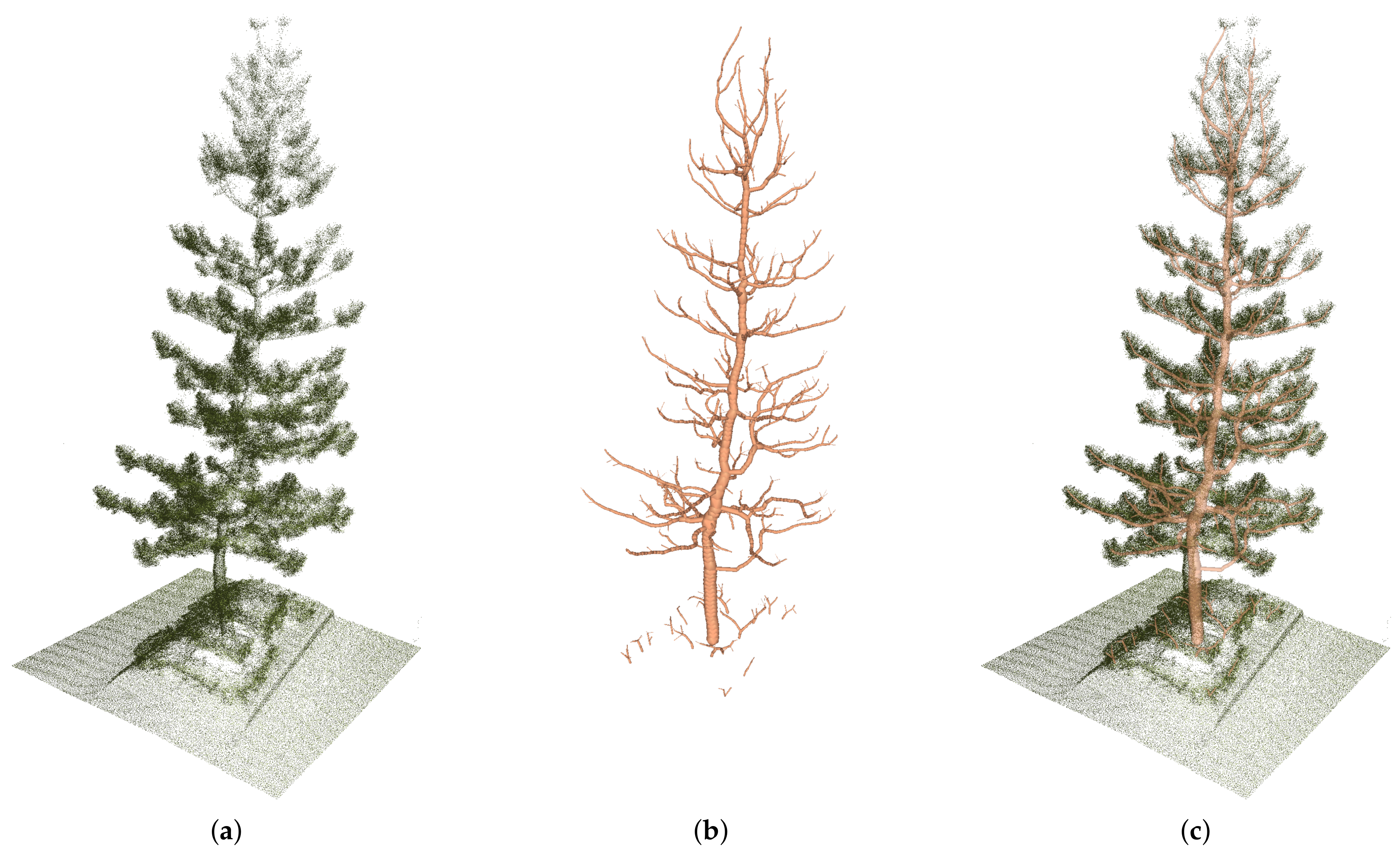
The results illustrate the efficacy of each stage of reconstruction, showing the distance between the density grid and the input point cloud, and the reconstructed BSG to the density grid. In the first five cases, in which there is minimal occlusion, the BSG reconstructs the observed trees with very high fidelity, capturing both large and small branches. Notably, it is also possible to see more thin branches in the BSG than in the thresholded density grid, demonstrating that the BSG reconstructs even low density details. This can be seen in Figure 6, which presents an enlarged view of case #1, its point cloud, BSG, and an overlaid view of the two. We highlight case #1 because the isolated pine tree is representative of managed plantations, in which tall and narrow trees are spaced on a regular grid, and because its features are clearly visible in the point cloud.
Several noteworthy features can be identified from the figure: firstly the square base in which the tree is planted is effectively removed by the optimisation. Whilst the optimisation treats everything in the raycloud as trees, its attempts to fit trees to the squat shape results in a set of small trunks near the ground. Secondly, the trunk and branches closely follow the visible limbs and have a diameter comparable to that in the point cloud. However, a few flaws are also noticeable: the lowest branch on the right of the tree emerges from the trunk far below the foliage, and at the top of the tree branches curve upwards erroneously to follow the surface, rather than the branches. These flaws likely arise from the low density of rays below the branches in the tree, the dense foliage at the top of the tree, and setting the branch angle parameter too low for the tree species.
In cases #2, #3 and #4 of Table 1, the denser foliage and close spacing of the Australian Eucalypts prevent TreeSep correctly segmenting them. In comparison, our method is able to both segment and reconstruct the trees to closely match the point clouds. In cases #3 and #4, part of another tree’s canopy is included in the dataset (and to a lesser extent in case #2). In cases #2 and #4, the partial canopy is clearly separated from other trees, and results in a spurious tree being constructed. The space where these tree trunks have formed should be filled with rays and therefore which would forbid woody material. The reason they form is that the ray cloud has been cropped to a width that is not a multiple of the voxel width w, and so the boundary voxels on the six faces of the grid are not fully filled with rays, which in these two cases has allowed sufficient woody material to form along the face to connect to the partial canopy. In case #3, the partial canopy is close to the foliage of the central tree. The topology optimisation produces a low-density connection to the main tree, which is cropped out during the BSG generation as the thin connection is below the minimum radius.
To explore these features in detail, we encourage readers to view the 3D point clouds and meshes available in the accompanying dataset.
Our method treats every point as part of a tree, and therefore it is clear from cases that include additional objects (cases #5, #7, #9) and lamp posts (#7, #14, #17) that non-tree objects would need to be classified and removed for best results.
Whilst these objects do not cause catastrophic failures, their presence does adversely affect the reconstruction. In the best case, these objects form spurious trees without affecting the real ones, as occurs with the shelter in case #5 and the lamp post in case #7. However, where the objects are close to, or overlapping with trees, they may become enmeshed in the tree’s BSG. This is most obvious in case #14, in which the lamp post is partially enclosed by the tree and is seen as part of the tree during optimisation.
It is evident that the algorithm generates tree-like structures that fit to this wide variety of point clouds, even in poorly distinguished foliage such as case #11. It is also clear from cases #7, #8 and #11 that our method is not reliant on a clearly distinguished trunk, and in case #6 the trunks are completely occluded by the overpass wall.
A key feature of this algorithm is that it uses the ray information to prevent trunks forming in observed free space. Given a sufficiently high density of rays, the voxel grid is implicitly classified as one of: known free space (where rays have passed without hitting anything), known occupied space (where the rays hit an object) or unknown space (when an occlusion prevents rays reaching the voxel). The optimisation is constrained to prevent material being located where voxels are determined to be free space. This is evident in case #10 where the free-space information prevents a trunk forming despite the canopy sitting very close to the ground (right hand side of the image).
As it does not rely on species specific features, our algorithm is able to reconstruct a broad range of tree types and features. For example in case #13, codominant stems are captured in the topology optimisation; however, during the BSG generation, most branches are joined back to the left stem. To be clear, whilst the method is capable of reconstructing a broad range of features, it performs best on a dataset with uniform branching angles, a well tuned and a dense raycloud.
The segmentation in the TreeSeparation algorithm is shown to approximately segment the main trees for the first four cases. However the remainder of cases are more densely overlapping trees, and the method severely underestimates the number of separate trees in each case. This is because TreeSeparation relies on a thinning or gap between neighbouring trees, which is barely present in cases #5 up to #13.
6.2. Quantitative Comparison: Table 3
In this section, we present a quantitative comparison for each case in Table 1 and Table 2, firstly as a Surface Error from the input point cloud, and secondly as a comparison of the number of identified trees to the two tree segmentation methods Treeseg [8] and TreeSeparation [12].
The voxel width w for each case is based on the number of voxels N and rounded to the nearest cm. As with any voxelisation of a point cloud, w can be varied, but is most effective when it is at a similar scale to the point density. Larger voxels underfit to the tree geometry, and smaller voxels overfit to gaps between the rays. The average in these experiments is cm which is approximately the point density at the more distant parts of the trees.
Across the 13 cases evaluated, SE averages to 15 cm or approximately two voxel widths. The lowest absolute errors are in the datasets optimised with a small voxel size w. However, the lowest relative errors () occur in the simpler tree cases. That is, the cases with fewer trees, more spacing between trees, an easily identifyable skeleton and minimal occlusions. Cases #1-5 all have an SE of less than 1.7 voxel widths, with the smallest being 1.2 for cases #3 and #4. In constrast, the complex and challenging cases with multiple overlapping trees, dense foliage, and other occlusions have a SE of 2.5–2.8 voxels. In terms of the number of trees produced, our algorithm matches the manual count within 13%, with our method erring on the side of too many stems.
While Treeseg and TreeSeparation both produce reasonable numbers of segments for the first five (well-separated) point clouds, TreeSeparation (which relies on gap features between trees) significantly underestimates the number of segments in the densely overlapping cases (#6 to #13) and Treeseg (which relies on trunk features) fails to process on the remaining datasets, which generally lack clear trunks.
6.3. Ablation Study: Table 4
This is a qualitative ablation study for comparing results with and without the convolution kernel, and respectively.
Here we can see the effect of the branch angle parameter on the reconstruction of heavily occluded trees. When the branches adhere close to the foliage surface in case #14 as that is the shortest path which joins the observed points to ground. The result is an unnatural looking set of surface branches. However, at , the larger branching angle forces branches to occupy the interior of the tree’s volume.
In cases #15, #16 and #18, the reconstruction generates a larger number of stems than the reconstruction. This is consistent with the expected behaviour of the branch angle parameter as demonstrated in two dimensions in Figure 3.
In case #18, three trees surround a small shrub in the centre on the image. At , trunks and primary branches of the three trees appear correctly located and sized, despite the absence of a central leader branch. However, the smaller shrub is poorly reconstructed. Because of the dense foliage, the reconstruction is unable to separate it from the surrounding trees.
In addition, at both and , the presence of a wall in the raycloud causes ‘trees’ to be generated to fit those points, resulting in the long branches on the left of the figure.
In case #16, the palm tree on the right of the figure is incorrectly reconstructed for both values of . This suggests that the branching structure of the palm fronds, which radiate from a central point, is inconsistent with the constant branch angle assumption of our method.
In case #19, the results for fit to the ray cloud better, which has long vertical stems on the left hand side. This is consistent with the data in Figure 3 that show that small better models vertical stems and narrow branch angles. Therefore, best results are expected when is set appropriately for the expected branch angle.
6.4. Aerial Comparison: Table 5
This is a qualitative comparison of a single tree that has been reconstructed from two different angles: a ground-based dense scan and sparse aerial scan.
In both cases, a full internal branch structure has been found that fits to the shape of the foliage. However the sparser aerial scan is biased towards a higher up branch structure, reflecting the relatively higher density on the top side of the tree. Additionally, the aerial scan is taken from a 45 downwards angle, giving a density distribution that favours an off-centre trunk. In both cases the internal branch structure is not observed in the scan.
6.5. Occlusion Study: Table 6
In this study, the sensitivity of the reconstruction to occlusion is estimated by simulating a spherical occlusion of varying sizes. Case #5 is selected for the study as it is representative of the unoccluded trees.
An occlusion is simulated by placing spheres at the geometric centre of each of the two trees in the dataset, removing all points from the point cloud that lie within the spheres. The ‘occluded’ trees are then reconstructed and their accuracy evaluated with varying sphere diameters.
The sphere diameters used are proportional to the trees’ height, and range from 1/8th of each tree’s height up to 1/2. The diameter of both trees’ spheres are increased simultaneously. In this experiment, the optimisation uses 1 million voxels, equating to a voxel size of 23 cm.
Small occlusions have little effect on the reconstruction, with a sphere 1/8th of the tree’s height leading to 3% increase in error. However, even with an occluding sphere diameter 3/8 of the tree height, which is approximately the diameter of each tree, the results show only a 61% error increase. Visually, we can see the unconstrained branch angle is greater than for the real tree, so smaller values of are likely to perform better for this tree species.
6.6. Voxel Size Sensitivity: Figure 5
The sensitivity of the reconstructed BSG surface error to the voxel size w is presented in Figure 5. As one would expect, the error increases roughly in proportion to the voxel size. There is a single outlier due to the BSG reconstruction phase missing a portion of one tree at the large voxel size of 36 cm. Other than this, the relationship is almost linear, with a best fit line at cm. There is an apparent slight levelling off at the smallest voxel sizes, which is expected behaviour when the voxel size becomes too small to be well-represented by lidar points. The levelling appears to occur from 20 cm wide voxels and lower, which corresponds to an average of 8 lidar points per occupied voxel.
Overall, the results demonstrate a well-behaved trade off between accuracy and solver resolution, with Surface Error approximately proportional to voxel width.
7. Physical Interpretation of Method
In this paper, we have used topology optimisation for the purely geometric purpose of interpolating lidar points with solid acyclic structures that reach the ground. However, Equation (2) also represents a physical system, where a quantity f distributes isotropically through each uniform element under the steady state equation . It is therefore possible to interpret the optimisation as a number of different physical processes that may be relevant in the formation of real trees:
- when f is rate of heat transfer and u is the change in temperature, E represents the thermal conductivity of the material. The optimisation therefore finds the structure that best conducts heat or cold away from the lidar points, this is the thermal model of topology optimisation.
- Equation (2) could be interpreted as approximating resistance to wind loading. The scalar load f represents an isotropic wind force, assuming the wind occurs equally in all directions over extended time periods. The parameter E is the Young’s modulus of the wood and u is the magnitude of position change. It therefore finds the structure that bends and moves least due to long term wind forces. This interpretation is aided by the fact that lidar points represent locations that a distant lidar can observe along straight rays. Which corresponds quite well with the set of locations that wind acts upon, namely the tree outer surfaces.
- in high foliage scans Equation (2) could approximate resistance to water loss. The load f represents the tensile force on water in the tree xylem due to transpiration at the leaf. The stiffness represents how easily water can be transported from the roots to the branches, and u represents the change in water content. It therefore finds the structure that minimises water loss from transpiration.
There are other similar approximations such as optimising the transport of sugars to the roots. In each case the physical process represents some form of load or effort at the lidar points that must be conducted efficiently to the ground.
The factors that affect tree structure remains an open topic of research, but we know that competition for light and resources favours trees that distribute their material efficiently, and this is a form of optimisation. Previously researched factors include wind load [53,54], efficiency and safety of hydraulic transport [55], and others such as stress minimisation in trees [56].
It is useful to consider such botanical interpretations because any future research that clarifies the optimising factors in tree structure can be used to extend the formulation in Equation (2), and so provide more accurate interpolation of branches in unobserved regions.
8. Limitations
The presented method has three limitations that remain to be addressed. Firstly, the total volume of the structure must be estimated a priori. We use the volume of occupied voxels as an estimator for this value but its estimation is still crude. Further research is required to better adapt the volume of material to the dataset being used.
Secondly, setting nodal load in proportion to number of lidar points is biased towards areas that are scanned for longer, or are observed at closer range. This bias is evident in the difference between the same tree, scanned in Table 5 from different directions. It is also evident in case 19, where the higher density of points on the right hand side cause the rightmost tree to ‘capture’ the canopy of all the trees. A simple improvement is to spatially subsample the ray cloud, and a more advanced technique could normalise the nodal loads to the mean load within a local neighbourhood.
Lastly, the four assumptions of our method in Section 1 are also forms of limitation. If clouds contain non-tree structures, cyclic structures, or trees with unobserved branches that are winding or at varying branch angles, then the method will not reconstruct these structures as they are. Instead, it will generate the tree structures that best fit its optimisation model.
It would be an instructive topic of future research to assess the severity of errors in the reconstruction due to data that break the above assumptions, and to assess the effect of improved nodal load distributions.
The focus on this paper has been on the method itself rather than its computational efficiency. We would therefore like to investigate the most optimal solver methods, software and parameters for solving Equation (2) as our next topic of research.
9. Conclusions
Methods of tree reconstruction in vegetated environments are hampered by the extreme variability of input data, and the lack of consistent features on which to segment trees or branches. Consequently, the majority of existing reconstruction techniques are limited to constrained environments, and suffer from catastrophic failures where the relied-on features are missing.
We have taken a radically different approach, avoiding feature-based reconstruction entirely, and instead treating the tree as the structure that matches the observed data while minimising compliance to loads. The results demonstrate the resilience of this simple minimisation rule under a wide range of datasets.
Our results suggest that topological optimisation is a valuable method for robust tree reconstruction, and deserves a prominent role in this field. They suggest that the research question should not focus on what are the features of a tree, but on what a tree optimises.
Author Contributions
Conceptualisation, T.L. and J.P.; methodology, T.L. and J.P.; software, T.L. and J.P.; validation, T.L. and J.P.; formal analysis, T.L. and J.P.; resources, T.L.; data curation, T.L. and J.P.; writing—original draft preparation, T.L. and J.P.; writing—review and editing, T.L. and J.P.; visualization, T.L. and J.P.; project administration, T.L.; funding acquisition, T.L. All authors have read and agreed to the published version of the manuscript.
Funding
This research was supported by Victorian Government’s Powerline Bushfire Safety Program R&D fund, Powercor, Sylvanus and CSIRO Data61.
Data Availability Statement
The datasets generated and used in the current study are available in the ‘Tree Reconstructions from Pointclouds Scanned in Pullenvale QLD’ repository https://doi.org/10.25919/yt2m-9373 (accessed on 16 October 2022).
Conflicts of Interest
The authors declare no conflict of interest.
Appendix A. Sensitivity
From Equation (2) the compliance for the smoothed densities can be expressed as a sum over all elements i:
where is defined in Equation (6) as the product of two terms. Using the product rule, the differential with respect to each smoothed element density can then be written as the sum of two terms:
where
and
The sensitivity with respect to the unsmoothed design variable is then:
where
References
- Trochta, J.; Krček, M.; Vrška, T.; Král, K. 3D Forest: An application for descriptions of three-dimensional forest structures using terrestrial LiDAR. PLoS ONE 2017, 12, e0176871. [Google Scholar] [CrossRef] [PubMed]
- Aiteanu, F.; Klein, R. Hybrid tree reconstruction from inhomogeneous point clouds. Vis. Comput. 2014, 30, 763–771. [Google Scholar] [CrossRef]
- Du, S.; Lindenbergh, R.; Ledoux, H.; Stoter, J.; Nan, L. AdTree: Accurate, detailed, and automatic modelling of laser-scanned trees. Remote Sens. 2019, 11, 2074. [Google Scholar] [CrossRef]
- Livny, Y.; Yan, F.; Olson, M.; Chen, B.; Zhang, H.; El-Sana, J. Automatic reconstruction of tree skeletal structures from point clouds. In Proceedings of the ACM SIGGRAPH Asia 2010, Seoul, Republic of Korea, 15–18 December 2010; pp. 1–8. [Google Scholar]
- Li, H.; Zhang, X.; Jaeger, M.; Constant, T. Segmentation of forest terrain laser scan data. In Proceedings of the 9th ACM SIGGRAPH Conference on Virtual-Reality Continuum and its Applications in Industry, Seoul, Republic of Korea, 12–13 December 2010; pp. 47–54. [Google Scholar]
- Zhong, L.; Cheng, L.; Xu, H.; Wu, Y.; Chen, Y.; Li, M. Segmentation of individual trees from TLS and MLS data. IEEE J. Sel. Top. Appl. Earth Obs. Remote Sens. 2016, 10, 774–787. [Google Scholar] [CrossRef]
- Liu, Q.; Ma, W.; Zhang, J.; Liu, Y.; Xu, D.; Wang, J. Point-cloud segmentation of individual trees in complex natural forest scenes based on a trunk-growth method. J. For. Res. 2021, 32, 2403–2414. [Google Scholar] [CrossRef]
- Burt, A.; Disney, M.; Calders, K. Extracting individual trees from lidar point clouds using treeseg. Methods Ecol. Evol. 2019, 10, 438–445. [Google Scholar] [CrossRef]
- Li, W.; Guo, Q.; Jakubowski, M.K.; Kelly, M. A new method for segmenting individual trees from the lidar point cloud. Photogramm. Eng. Remote Sens. 2012, 78, 75–84. [Google Scholar] [CrossRef]
- Ayrey, E.; Fraver, S.; Kershaw Jr, J.A.; Kenefic, L.S.; Hayes, D.; Weiskittel, A.R.; Roth, B.E. Layer stacking: A novel algorithm for individual forest tree segmentation from LiDAR point clouds. Can. J. Remote Sens. 2017, 43, 16–27. [Google Scholar] [CrossRef]
- Heinzel, J.; Huber, M.O. Constrained spectral clustering of individual trees in dense forest using terrestrial laser scanning data. Remote Sens. 2018, 10, 1056. [Google Scholar] [CrossRef]
- Wang, J.; Lindenbergh, R.; Menenti, M. Scalable individual tree delineation in 3D point clouds. Photogramm. Rec. 2018, 33, 315–340. [Google Scholar] [CrossRef]
- Luo, H.; Khoshelham, K.; Chen, C.; He, H. Individual tree extraction from urban mobile laser scanning point clouds using deep pointwise direction embedding. ISPRS J. Photogramm. Remote Sens. 2021, 175, 326–339. [Google Scholar] [CrossRef]
- Krisanski, S.; Taskhiri, M.S.; Aracil, S.G.; Herries, D.; Turner, P. Sensor agnostic semantic segmentation of structurally diverse and complex forest point clouds using deep learning. Remote Sens. 2021, 13, 1413. [Google Scholar] [CrossRef]
- Tagliasacchi, A.; Delame, T.; Spagnuolo, M.; Amenta, N.; Telea, A. 3d skeletons: A state-of-the-art report. In Proceedings of the Computer Graphics Forum, Berlin, Germany, 20–24 June 2016; Volume 35, pp. 573–597. [Google Scholar]
- Schilling, A.; Maas, H.G. Automatic Reconstruction of Skeletal Structures from TLS Forest Scenes. ISPRS Ann. Photogramm. Remote Sens. Spat. Inf. Sci. 2014, 2, 321–328. [Google Scholar] [CrossRef]
- Jiang, A.; Liu, J.; Zhou, J.; Zhang, M. Skeleton extraction from point clouds of trees with complex branches via graph contraction. Vis. Comput. 2020, 37, 1–17. [Google Scholar] [CrossRef]
- Raumonen, P.; Kaasalainen, M.; Åkerblom, M.; Kaasalainen, S.; Kaartinen, H.; Vastaranta, M.; Holopainen, M.; Disney, M.; Lewis, P. Fast automatic precision tree models from terrestrial laser scanner data. Remote Sens. 2013, 5, 491–520. [Google Scholar] [CrossRef]
- Wang, R.; Peethambaran, J.; Chen, D. Lidar point clouds to 3-D urban models: A review. IEEE J. Sel. Top. Appl. Earth Obs. Remote Sens. 2018, 11, 606–627. [Google Scholar] [CrossRef]
- Hu, S.; Li, Z.; Zhang, Z.; He, D.; Wimmer, M. Efficient tree modeling from airborne LiDAR point clouds. Comput. Graph. 2017, 67, 1–13. [Google Scholar] [CrossRef]
- Xu, H.; Gossett, N.; Chen, B. Knowledge and heuristic-based modeling of laser-scanned trees. ACM Trans. Graph. (TOG) 2007, 26, 19-es. [Google Scholar] [CrossRef]
- Raumonen, D.P. TreeQSM. 2017. Available online: https://github.com/InverseTampere/TreeQSM (accessed on 16 October 2022).
- Fan, G.; Nan, L.; Dong, Y.; Su, X.; Chen, F. AdQSM: A New Method for Estimating Above-Ground Biomass from TLS Point Clouds. Remote Sens. 2020, 12, 3089. [Google Scholar] [CrossRef]
- Ikonen, T.J.; Marck, G.; Sóbester, A.; Keane, A.J. Topology optimization of conductive heat transfer problems using parametric L-systems. Struct. Multidiscip. Optim. 2018, 58, 1899–1916. [Google Scholar] [CrossRef]
- Pinskier, J.; Shirinzadeh, B.; Ghafarian, M.; Das, T.K.; Al-Jodah, A.; Nowell, R. Topology optimization of stiffness constrained flexure-hinges for precision and range maximization. Mech. Mach. Theory 2020, 150, 103874. [Google Scholar] [CrossRef]
- Pinskier, J.; Shirinzadeh, B. Topology optimization of leaf flexures to maximize in-plane to out-of-plane compliance ratio. Precis. Eng. 2019, 55, 397–407. [Google Scholar] [CrossRef]
- Clark, L.; Shirinzadeh, B.; Pinskier, J.; Tian, Y.; Zhang, D. Topology optimisation of bridge input structures with maximal amplification for design of flexure mechanisms. Mech. Mach. Theory 2018, 122, 113–131. [Google Scholar] [CrossRef]
- Pinskier, J.; Howard, D. From Bioinspiration to Computer Generation: Developments in Autonomous Soft Robot Design. Adv. Intell. Syst. 2022, 4, 2100086. [Google Scholar] [CrossRef]
- Zhang, H.; Kumar, A.S.; Fuh, J.Y.H.; Wang, M.Y. Design and Development of a Topology-Optimized Three-Dimensional Printed Soft Gripper. Soft Robot. 2018, 5, 650–661. [Google Scholar] [CrossRef]
- Sigmund, O. Design of multiphysics actuators using topology optimization - Part I: One-material structures. Comput. Methods Appl. Mech. Eng. 2001, 190, 6605–6627. [Google Scholar] [CrossRef]
- Kumar, P.; Frouws, J.S.; Langelaar, M. Topology optimization of fluidic pressure-loaded structures and compliant mechanisms using the Darcy method. Struct. Multidiscip. Optim. 2020, 61, 1637–1655. [Google Scholar] [CrossRef]
- Munk, D.J.; Kipouros, T.; Vio, G.A.; Steven, G.P.; Parks, G.T. Topology optimisation of micro fluidic mixers considering fluid-structure interactions with a coupled Lattice Boltzmann algorithm. J. Comput. Phys. 2017, 349, 11–32. [Google Scholar] [CrossRef]
- Zhang, H.K.; Zhou, J.; Fang, W.; Zhao, H.; Zhao, Z.L.; Chen, X.; Zhao, H.P.; Feng, X.Q. Multi-functional topology optimization of Victoria cruziana veins. J. R. Soc. Interface 2022, 19. [Google Scholar] [CrossRef]
- Bendsøe, M.P.; Sigmund, O. Topology Optimization: Theory, Methods, and Applications; Springer: Berlin/Heidelberg, Germany, 2003; p. 370. [Google Scholar] [CrossRef]
- Zhang, X.; Zhu, B. Topology Optimization of Compliant Mechanisms; Springer: Berlin/Heidelberg, Germany, 2018; pp. 1–192. [Google Scholar]
- Sigmund, O.; Maute, K. Topology optimization approaches: A comparative review. Struct. Multidiscip. Optim. 2013, 48, 1031–1055. [Google Scholar] [CrossRef]
- Munk, D.J.; Vio, G.A.; Steven, G.P. Topology and shape optimization methods using evolutionary algorithms: A review. Struct. Multidiscip. Optim. 2015, 52, 613–631. [Google Scholar] [CrossRef]
- Van Dijk, N.P.; Maute, K.; Langelaar, M.; Van Keulen, F. Level-set methods for structural topology optimization: A review. Struct. Multidiscip. Optim. 2013, 48, 437–472. [Google Scholar] [CrossRef]
- Yuta, T. PANSFEM. 2019. Available online: https://github.com/PANFACTORY/PANSFEM2 (accessed on 16 October 2022).
- Andreassen, E.; Clausen, A.; Schevenels, M.; Lazarov, B.S.; Sigmund, O. Efficient topology optimization in MATLAB using 88 lines of code. Struct. Multidiscip. Optim. 2011, 43, 1–16. [Google Scholar] [CrossRef]
- Guest, J.K.; Prévost, J.H.; Belytschko, T. Achieving minimum length scale in topology optimization using nodal design variables and projection functions. Int. J. Numer. Methods Eng. 2004, 61, 238–254. [Google Scholar] [CrossRef]
- Liu, C.H.; Chen, Y.; Yang, S.Y. Topology Optimization and Prototype of a Multimaterial-Like Compliant Finger by Varying the Infill Density in 3D Printing. Soft Robot. 2021, 9, 212. [Google Scholar] [CrossRef]
- Fleury, C. CONLIN: An efficient dual optimizer based on convex approximation concepts. Struct. Optim. 1989, 1, 81–89. [Google Scholar] [CrossRef]
- Yan, S.; Wang, F.; Sigmund, O. On the non-optimality of tree structures for heat conduction. Int. J. Heat Mass Transf. 2018, 122, 660–680. [Google Scholar] [CrossRef]
- Lowe, T.; Stepanas, K. RayCloudTools: A Concise Interface for Analysis and Manipulation of Ray Clouds. IEEE Access 2021, 9, 79712–79724. [Google Scholar] [CrossRef]
- Calders, K.; Newnham, G.; Burt, A.; Murphy, S.; Raumonen, P.; Herold, M.; Culvenor, D.; Avitabile, V.; Disney, M.; Armston, J.; et al. Nondestructive estimates of above-ground biomass using terrestrial laser scanning. Methods Ecol. Evol. 2015, 6, 198–208. [Google Scholar] [CrossRef]
- Dijkstra, E.W. A note on two problems in connexion with graphs. Numer. Math. 1959, 1, 269–271. [Google Scholar] [CrossRef]
- Ramezani, M.; Khosoussi, K.; Catt, G.; Moghadam, P.; Williams, J.; Borges, P.; Pauling, F.; Kottege, N. Wildcat: Online Continuous-Time 3D Lidar-Inertial SLAM. arXiv, 2022; arXiv:2205.12595. [Google Scholar]
- Wang, J. TreeSeparation. 2020. Available online: https://github.com/Jinhu-Wang/TreeSeparation (accessed on 16 October 2022).
- Burt, A.; Peter, T. Jgrn307. Apburt/Treeseg: V0.2.2. 2021. Available online: https://zenodo.org/record/4884923#.Y6wNfUxByHs (accessed on 16 October 2022).
- Westling, F.; Bryson, M.; Underwood, J. SimTreeLS: Simulating aerial and terrestrial laser scans of trees. Comput. Electron. Agric. 2021, 187, 106277. [Google Scholar] [CrossRef]
- Esmorís, A.M.; Yermo, M.; Weiser, H.; Winiwarter, L.; Höfle, B.; Rivera, F.F. Virtual LiDAR Simulation as a High Performance Computing Challenge: Toward HPC HELIOS++. IEEE Access 2022, 10, 105052–105073. [Google Scholar] [CrossRef]
- Eloy, C.; Fournier, M.; Lacointe, A.; Moulia, B. Wind loads and competition for light sculpt trees into self-similar structures. Nat. Commun. 2017, 8, 1014. [Google Scholar] [CrossRef] [PubMed]
- Eloy, C. Leonardo’s rule, self-similarity, and wind-induced stresses in trees. Phys. Rev. Lett. 2011, 107, 258101. [Google Scholar] [CrossRef]
- Midgley, J.J. Is bigger better in plants? The hydraulic costs of increasing size in trees. Trends Ecol. Evol. 2003, 18, 5–6. [Google Scholar] [CrossRef]
- Mattheck, C.; Tesari, I. The mechanical self-optimisation of trees. WIT Trans. Ecol. Environ. 2004, 73, 197–206. [Google Scholar]
Figure 1.
A reconstruction of a challenging, cluttered environment where all tree bases are occluded and approximately 2 m below the overpass. It shows the overlaid view of point cloud (green) and generated trees (blue).
Figure 1.
A reconstruction of a challenging, cluttered environment where all tree bases are occluded and approximately 2 m below the overpass. It shows the overlaid view of point cloud (green) and generated trees (blue).

Figure 2.
Two-dimensional depiction of our method. From left to right: ray cloud and ground mesh of a natural scene, optimiser constraints, optimiser output (per-voxel wood density), and BSG. The optimiser constraints are the Dirichlet condition (red dots), Neumann condition (green dots), and the maximum volume condition (white = 1, orange = 0) as defined in Equation (2).

Figure 3.
Convolution with radial reciprocal kernel shown in green, for branch angle parameter (left to right). The resulting tree from five point loads is shown in white.
Figure 3.
Convolution with radial reciprocal kernel shown in green, for branch angle parameter (left to right). The resulting tree from five point loads is shown in white.

Figure 4.
Dijkstra’s algorithm on a 2D three-point tree, using density-scaled distance function, and segmented by Euclidean path distance every two element widths. Brightness is pseudodensity. White points are the density-weighted centroids of each contiguous segment, which form the nodes of the Branch Structure Graph.

Figure 5.
Sensitivity of Surface Error to the voxel size w for case #5 with non-tree objects removed.
Figure 5.
Sensitivity of Surface Error to the voxel size w for case #5 with non-tree objects removed.

Figure 6.
Enlarged view of lone pine tree (case #1). (a) Closeup view of point cloud (b) Reconstructed BSG (c) Overlaid view of BSG on point cloud.
Figure 6.
Enlarged view of lone pine tree (case #1). (a) Closeup view of point cloud (b) Reconstructed BSG (c) Overlaid view of BSG on point cloud.


Table 1.
Qualitative results (Part 1), showing the original point cloud, topology optimised voxel representation of the tree, and the reconstructed branch structure graph. The segmented trees produced by TreeSep [12] are presented for comparison.
Table 1.
Qualitative results (Part 1), showing the original point cloud, topology optimised voxel representation of the tree, and the reconstructed branch structure graph. The segmented trees produced by TreeSep [12] are presented for comparison.
| Case | Point Cloud | Voxelised Result | BSG | TreeSep |
|---|---|---|---|---|
| 1 Single tree |  |  |  |  |
| 2 Two trees |  |  |  |  |
| 3 Partial tree canopy on left |  |  |  |  |
| 4 Partial tree canopy on right |  |  |  |  |
| 5 Trees and shelter |  |  |  |  |
| 6 Trunks occluded behind overpass |  |  |  |  |
Table 2.
Qualitative results (Part 2), showing the original point cloud, topology optimised voxel representation of the tree, and the reconstructed branch structure graph. The segmented trees produced by TreeSep [12] are presented for comparison.
Table 2.
Qualitative results (Part 2), showing the original point cloud, topology optimised voxel representation of the tree, and the reconstructed branch structure graph. The segmented trees produced by TreeSep [12] are presented for comparison.
| Case | Point Cloud | Voxelised Result | BSG | TreeSep |
|---|---|---|---|---|
| 7 Trunk covered in vegetation |  |  |  |  |
| 8 Trunk occluded by vegetation |  |  |  |  |
| 9 Viewed on one side. Wall visible |  |  |  |  |
| 10 Canopy reaches almost to ground |  |  |  |  |
| 11 Overlapping vegetation |  |  |  |  |
| 12 Overlapping, close proximity trees |  |  |  |  |
| 13 non-singular, split trunk |  |  |  |  |
Table 3.
Quantitative comparison. For each case in Table 1 and Table 2 and we present the Surface Error (SE) of our method to its point cloud, and compare the principle number of stems reconstructed with the number of segments produced from the popular Treeseg and TreeSeparation algorithms. Failed functions are marked with ✗.
| Case | w (cm) | SE (cm) | SE/w | Estimated Cloud #segs | Our Method #segs | Treeseg #segs | TreeSeparation #segs |
|---|---|---|---|---|---|---|---|
| 1 | 6 | 9.9 | 1.7 | 1 | 1 | ✗ | 1 |
| 2 | 13 | 18.9 | 1.5 | 2 | 4 | 2 | 2 |
| 3 | 16 | 18.6 | 1.2 | 3 | 4 | 1 | 2 |
| 4 | 14 | 16.4 | 1.2 | 2 | 3 | 2 | 4 |
| 5 | 13 | 21.0 | 1.6 | 2 | 4 | 1 | 3 |
| 6 | 5 | 12.7 | 2.5 | 10 | 11 | ✗ | 2 |
| 7 | 10 | 17.8 | 1.8 | 7 | 8 | ✗ | 2 |
| 8 | 9 | 16.6 | 1.8 | 5 | 4 | ✗ | 2 |
| 9 | 5 | 10.6 | 2.1 | 4 | 5 | ✗ | 1 |
| 10 | 5 | 13.6 | 2.7 | 6 | 8 | ✗ | 1 |
| 11 | 6 | 16.9 | 2.8 | 10 | 8 | ✗ | 2 |
| 12 | 6 | 13.1 | 2.2 | 9 | 9 | ✗ | 1 |
| 13 | 4 | 10.7 | 2.7 | 1 | 1 | ✗ | 1 |
| mean | 8.6 cm | 15.1 | 2.0 | 4.8 | 5.4 | - | 1.8 |
Table 4.
Ablation study: comparing results for two values of the branch angle parameter on dense foliage that heavily restricts branch visibility.
Table 4.
Ablation study: comparing results for two values of the branch angle parameter on dense foliage that heavily restricts branch visibility.
| Problem Case | Point Cloud | BSG | BSG |
|---|---|---|---|
| 14 Dense canopy occludes all branches |  |  |  |
| 15 Flat top |  |  |  |
| 16 Thickly overlapping including palm |  |  |  |
| 17 Thick foliage occludes branches |  |  |  |
| 18 tree tucked under others. Wall visible |  |  |  |
| 19 Steep ground, undergrowth |  |  |  |
Table 5.
Aerial comparison: of a tree reconstructed from high-density ground data and sparse aerial data of a Moreton Bay fig tree.
Table 5.
Aerial comparison: of a tree reconstructed from high-density ground data and sparse aerial data of a Moreton Bay fig tree.
| Problem Case | Point Cloud | BSG | Superimposed |
|---|---|---|---|
| 20 Thick Foliage Ground Scan |  |  |  |
| 21 Thick Foliage Aerial Scan |  |  |  |
Table 6.
Occlusion study: the optimisation procedure is repeated after removing spheres ranging in diameter from 1/8 to 1/2 of each trees height (red) from their geometric centre, replicating an occlusion. Even with a significant proportion of point removed from the cloud, little change is observed in the reconstructed trees (blue).
| Removed Sphere Diameter (Relative to Tree Height) | |||||
|---|---|---|---|---|---|
| Test Case | Original Point Cloud | 1/8 | 2/8 | 3/8 | 4/8 |
| SE (cm) | 20.3 | 20.9 | 24.5 | 32.7 | 49.0 |
| SE/w | 0.9 | 0.9 | 1.1 | 1.4 | 2.1 |
 |  |  |  |  | |
Disclaimer/Publisher’s Note: The statements, opinions and data contained in all publications are solely those of the individual author(s) and contributor(s) and not of MDPI and/or the editor(s). MDPI and/or the editor(s) disclaim responsibility for any injury to people or property resulting from any ideas, methods, instructions or products referred to in the content. |
© 2022 by the authors. Licensee MDPI, Basel, Switzerland. This article is an open access article distributed under the terms and conditions of the Creative Commons Attribution (CC BY) license (https://creativecommons.org/licenses/by/4.0/).
Share and Cite
MDPI and ACS Style
Lowe, T.; Pinskier, J. Tree Reconstruction Using Topology Optimisation. Remote Sens. 2023, 15, 172. https://doi.org/10.3390/rs15010172
AMA Style
Lowe T, Pinskier J. Tree Reconstruction Using Topology Optimisation. Remote Sensing. 2023; 15(1):172. https://doi.org/10.3390/rs15010172
Chicago/Turabian StyleLowe, Thomas, and Joshua Pinskier. 2023. "Tree Reconstruction Using Topology Optimisation" Remote Sensing 15, no. 1: 172. https://doi.org/10.3390/rs15010172
Note that from the first issue of 2016, this journal uses article numbers instead of page numbers. See further details here.