

Geostationary Full-Spectrum Wide-Swath High-Fidelity Imaging Spectrometer: Optical Design and Prototype Development
 , ,
, ,
Abstract
:
1. Introduction
2. Principle and Method
3. Optical Design and Analysis
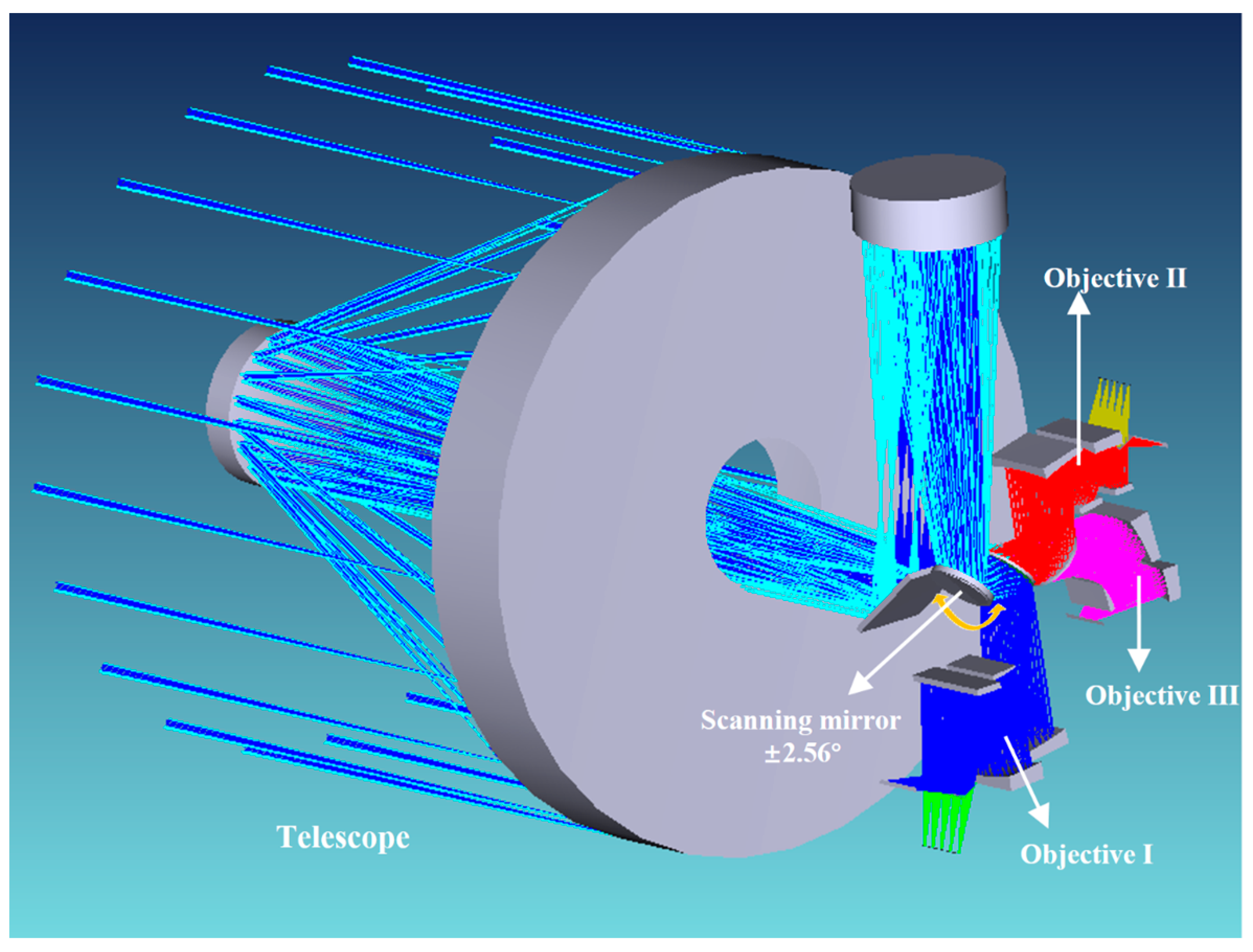
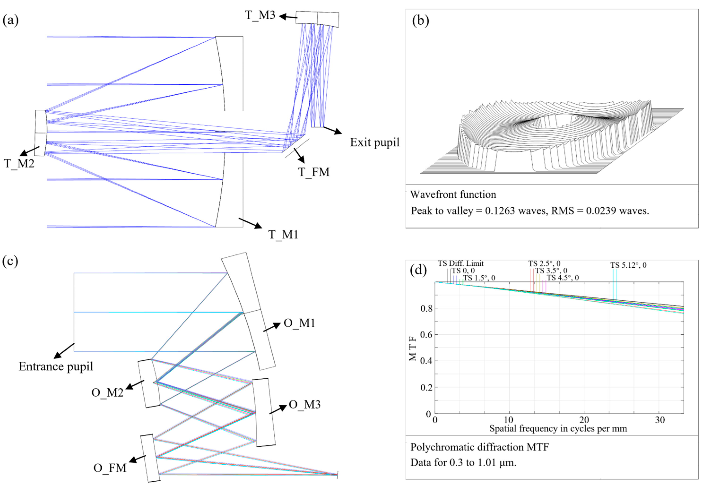
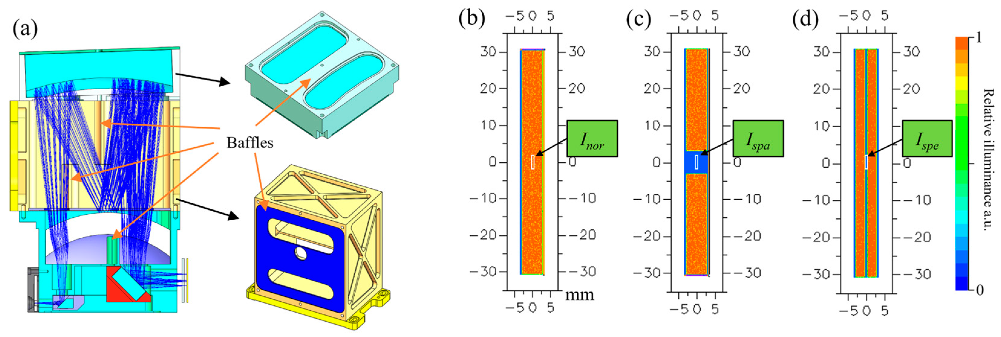
3.1. Fore-Optics
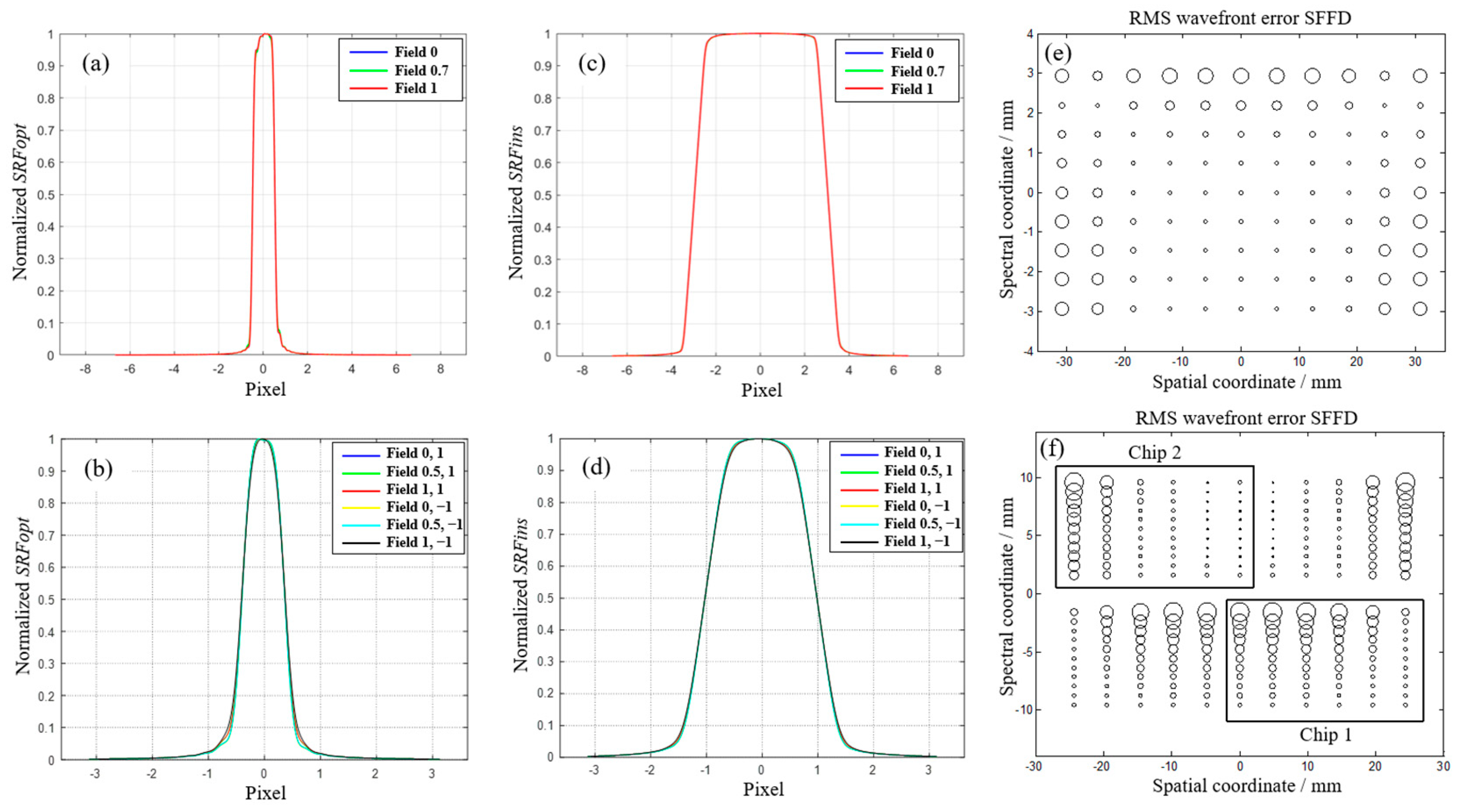
3.2. High-Fidelity Spectrometers

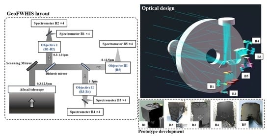
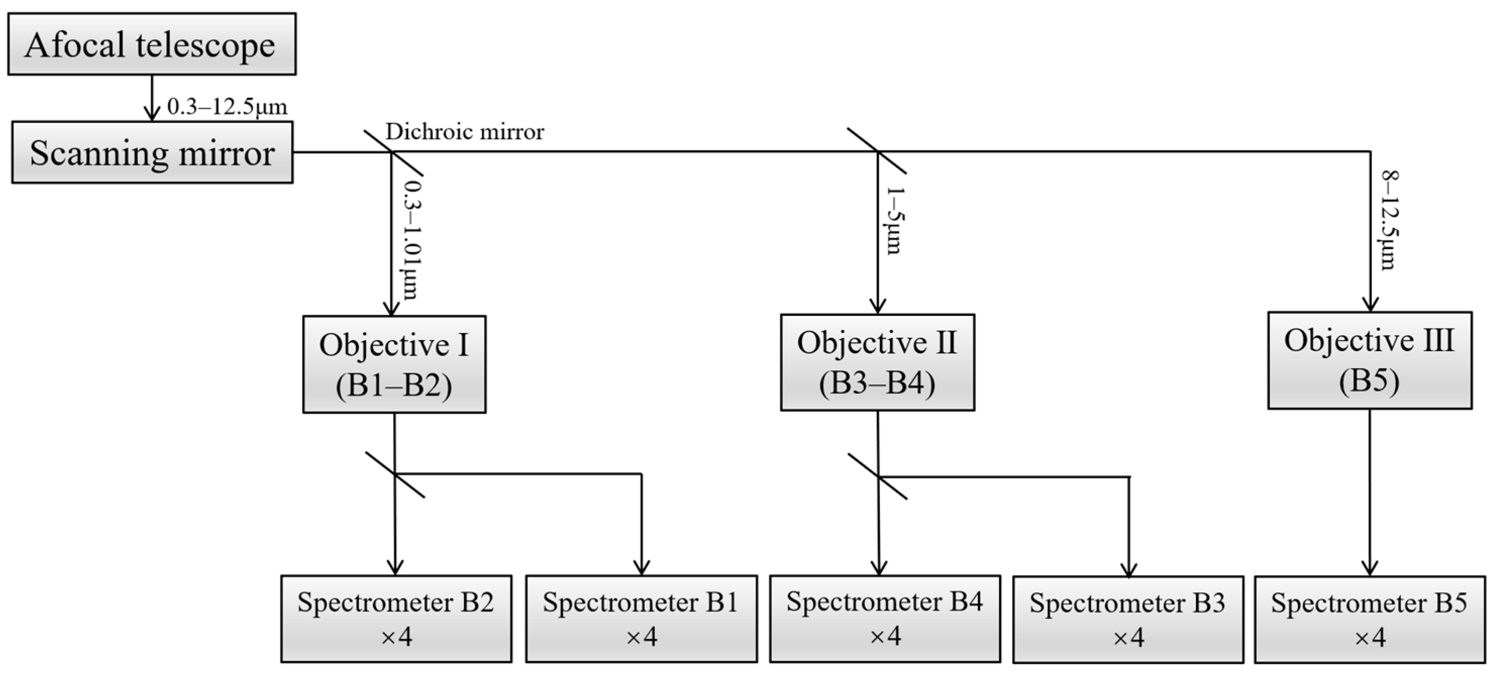
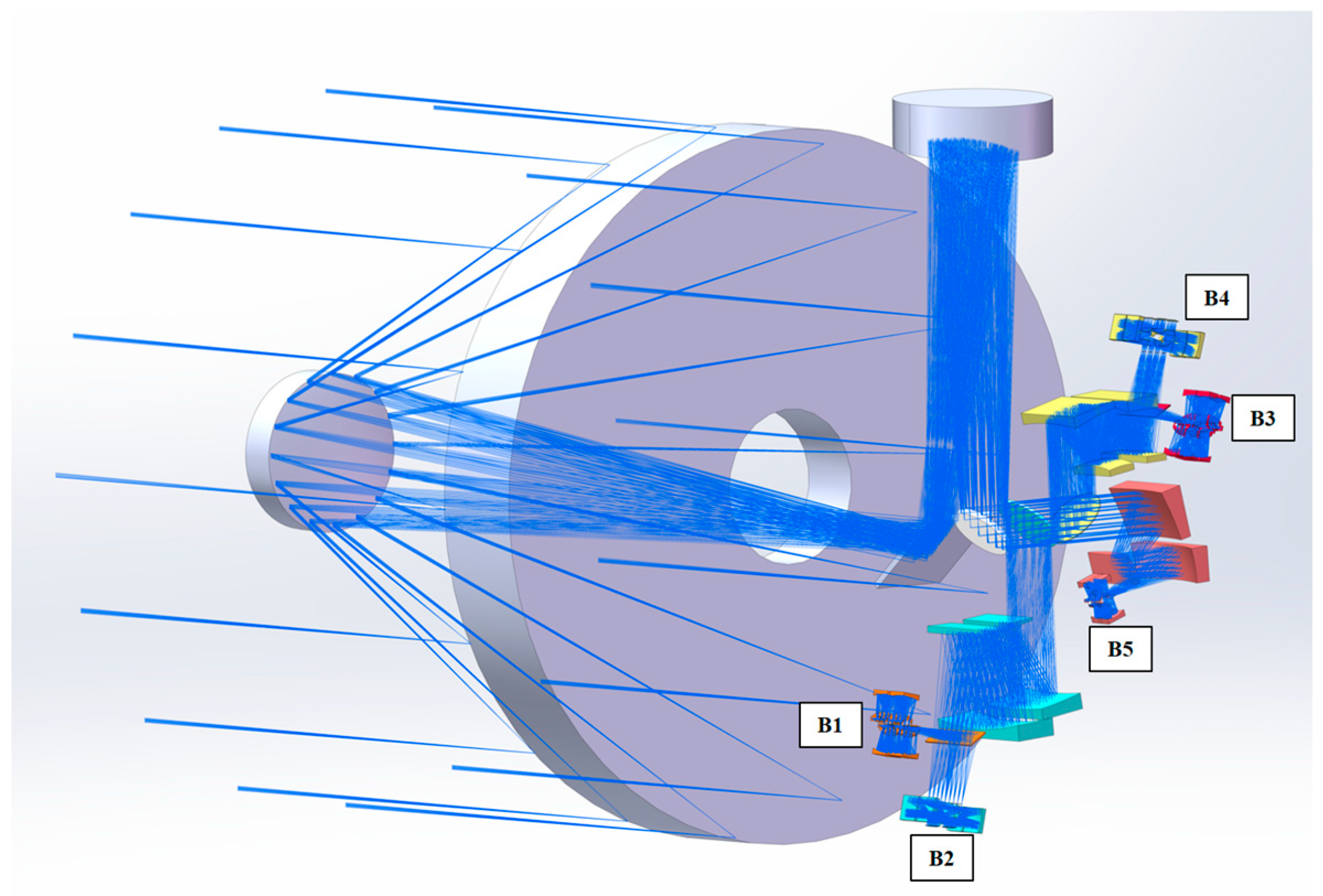
3.3. Optical System of GeoFWHIS
4. Experiment Results
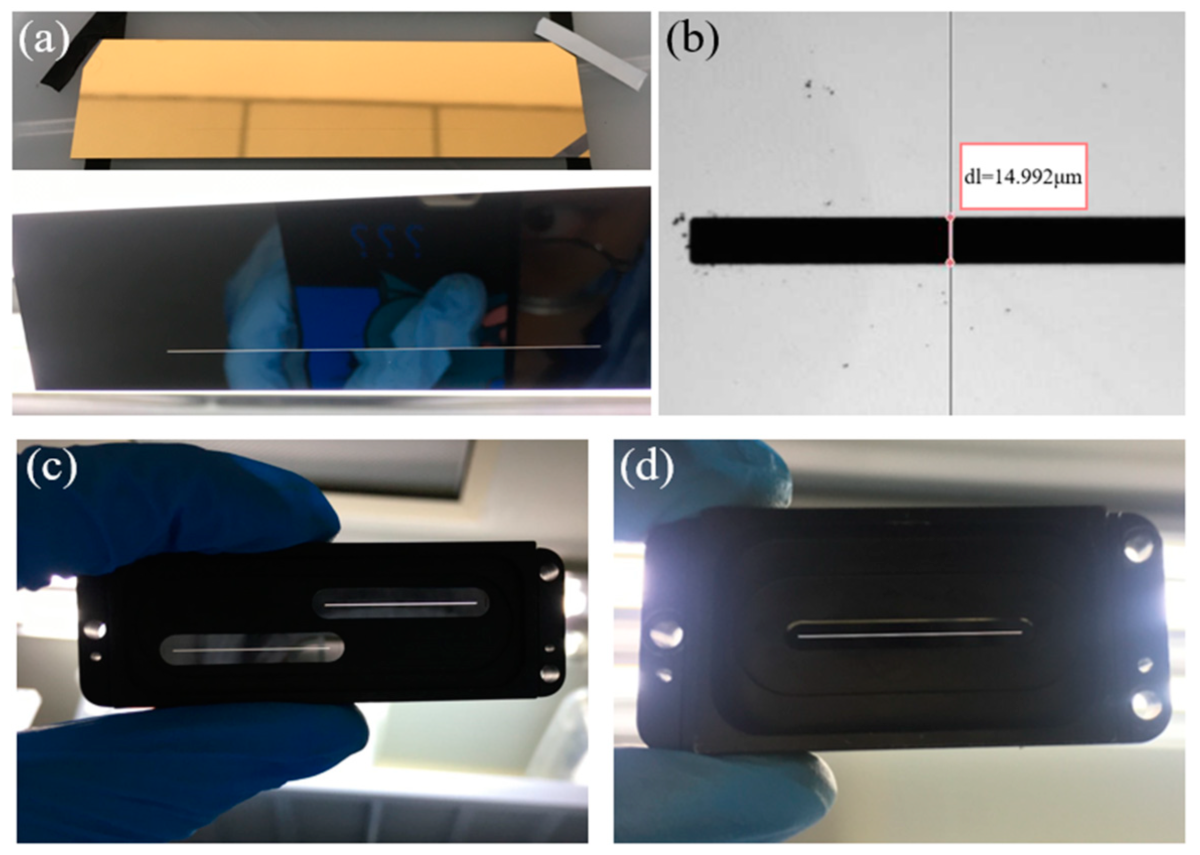
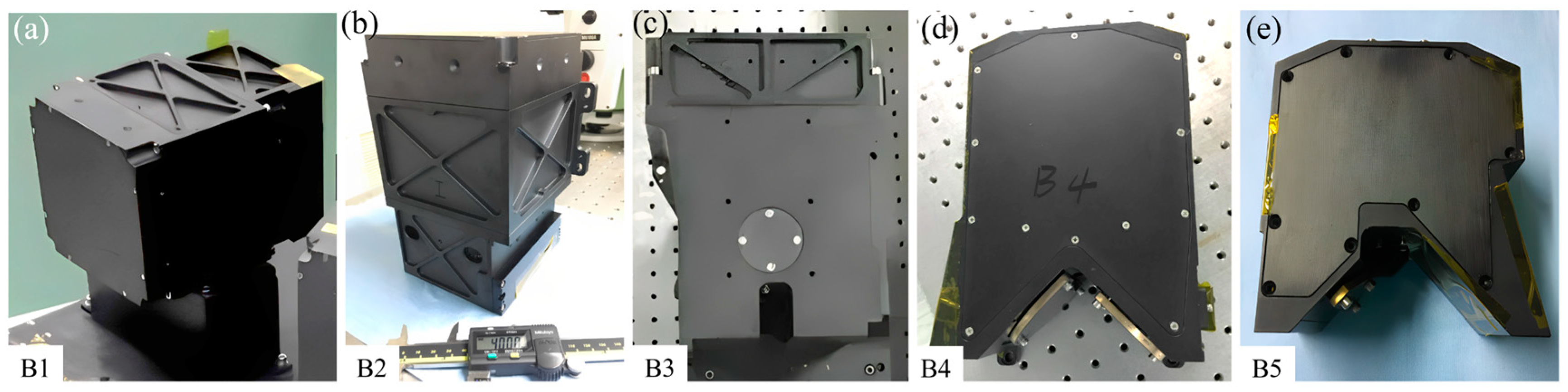
4.1. Manufacture of Slits and Gratings
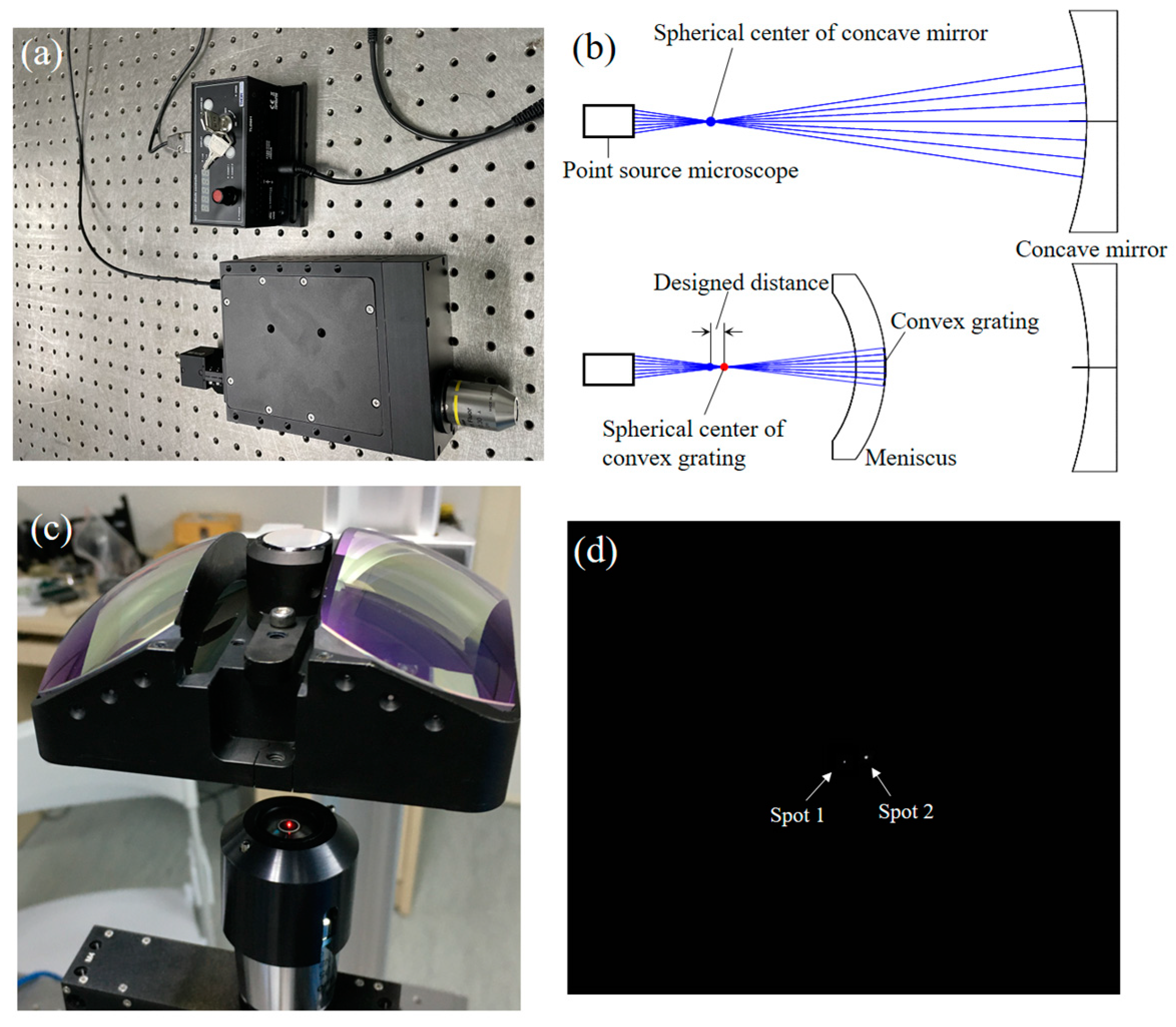
4.2. Alignment
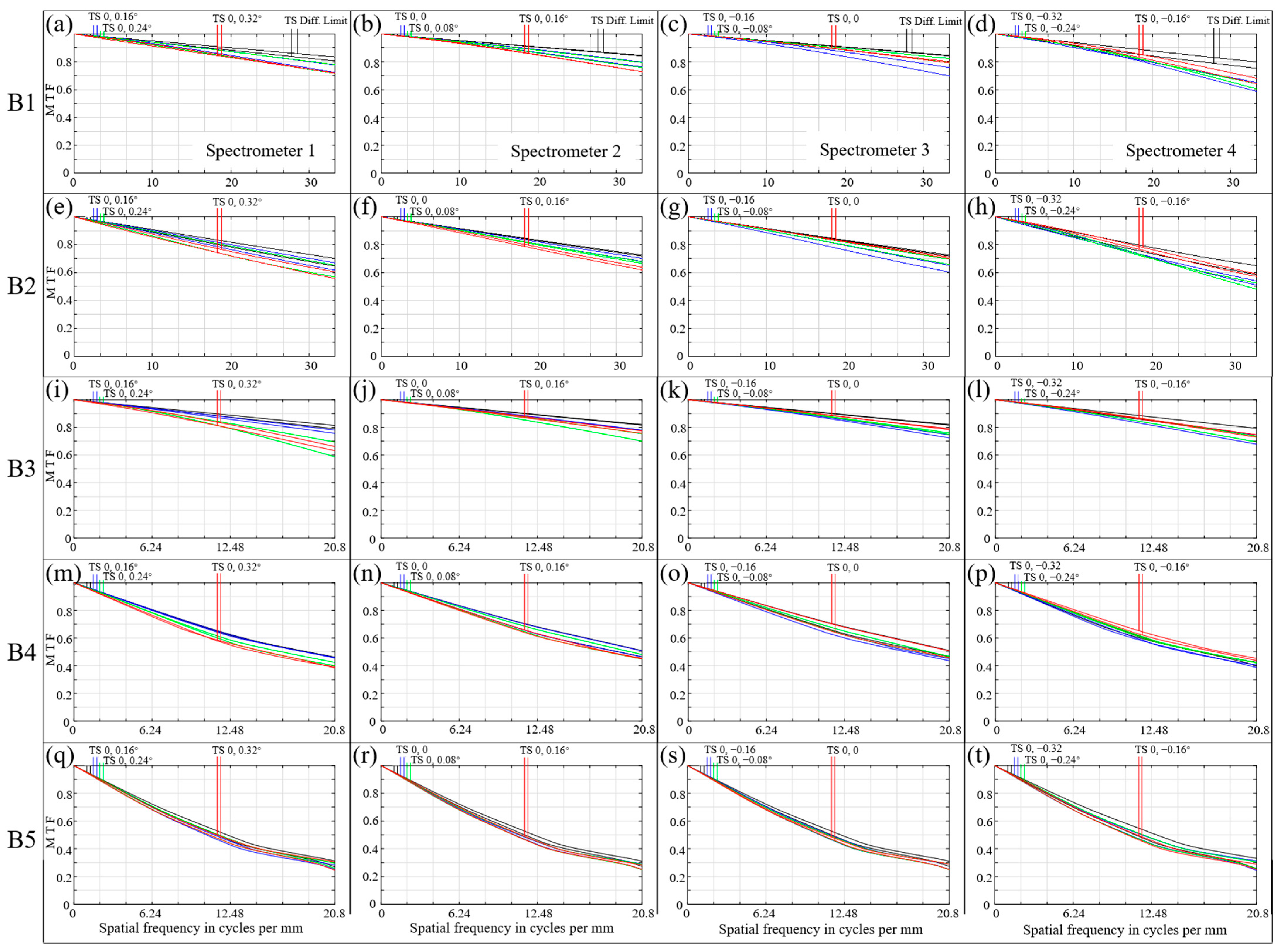
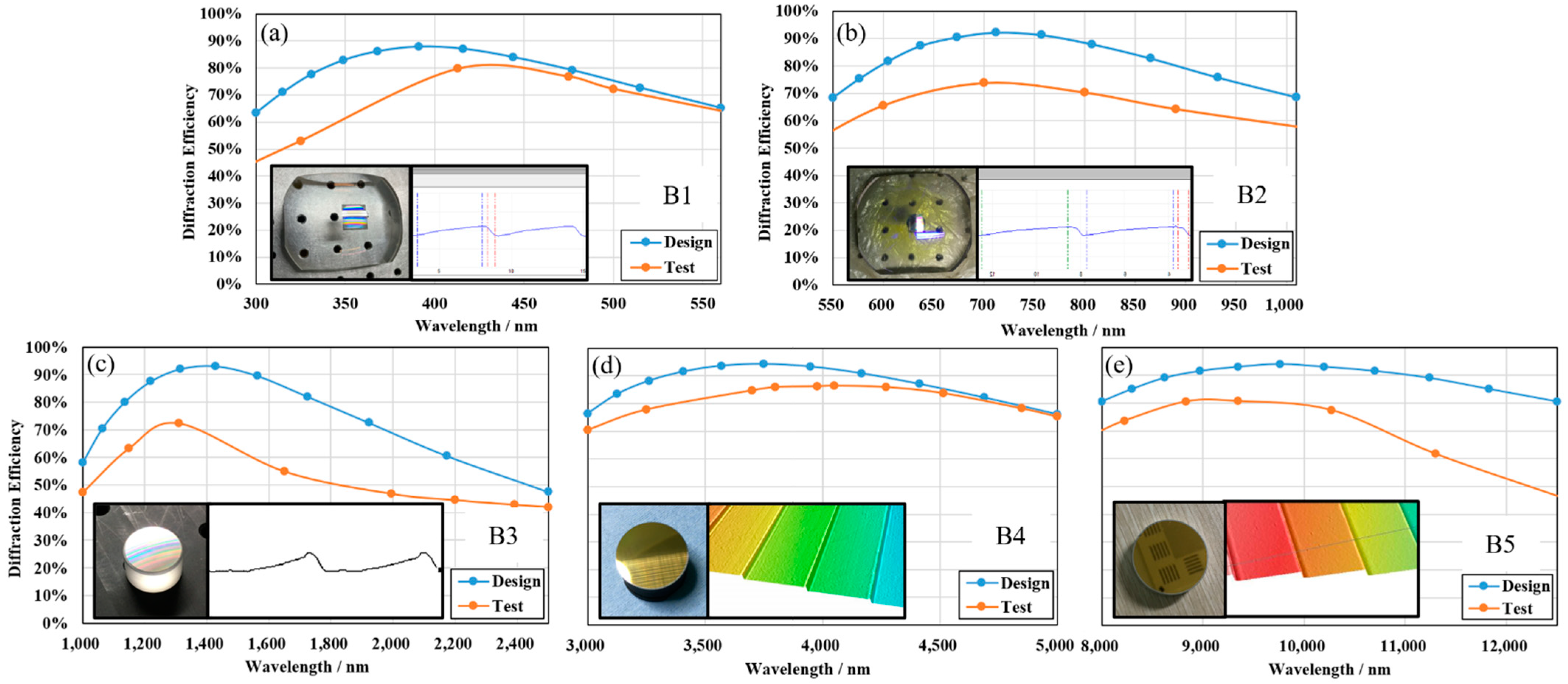
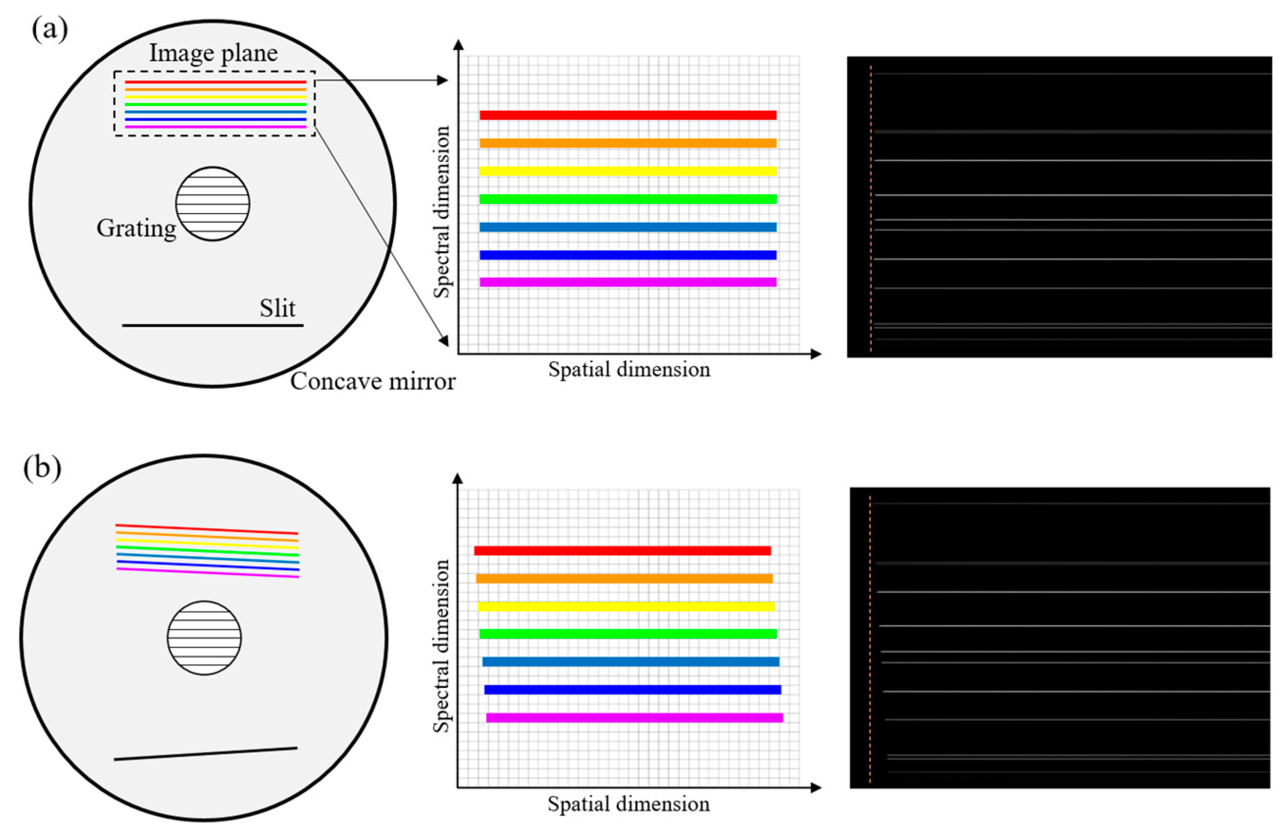
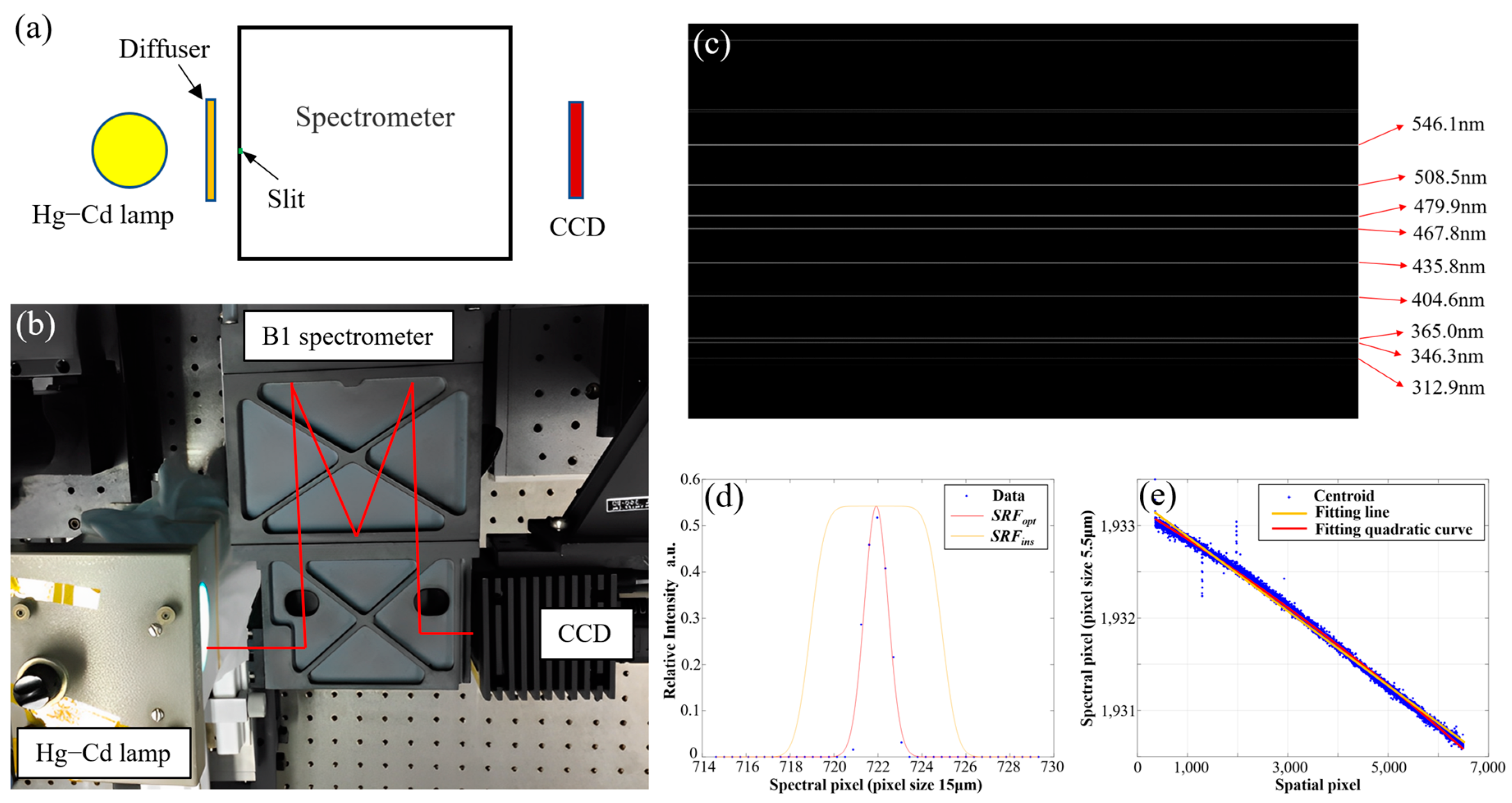
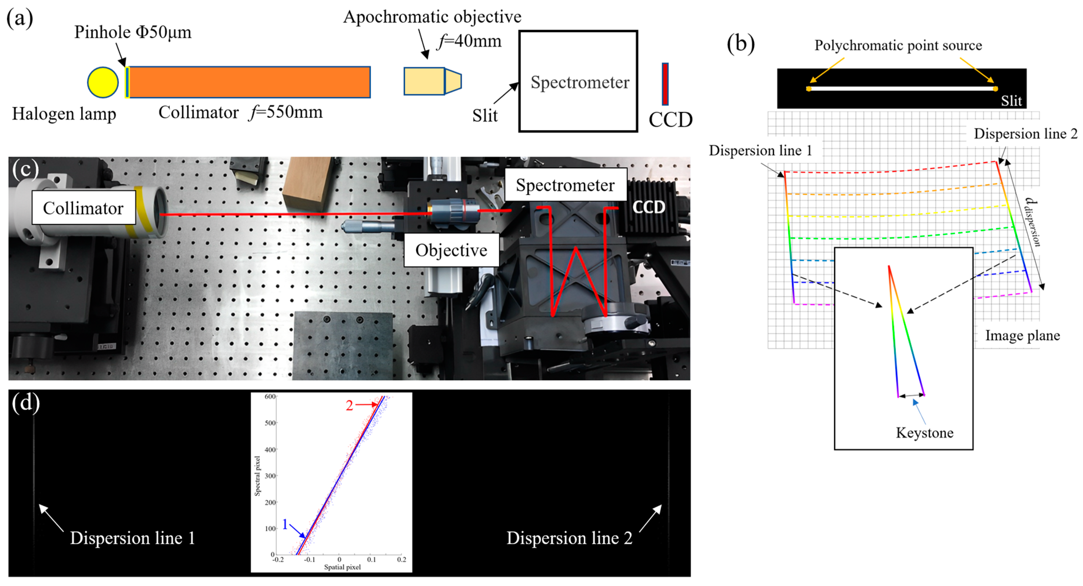
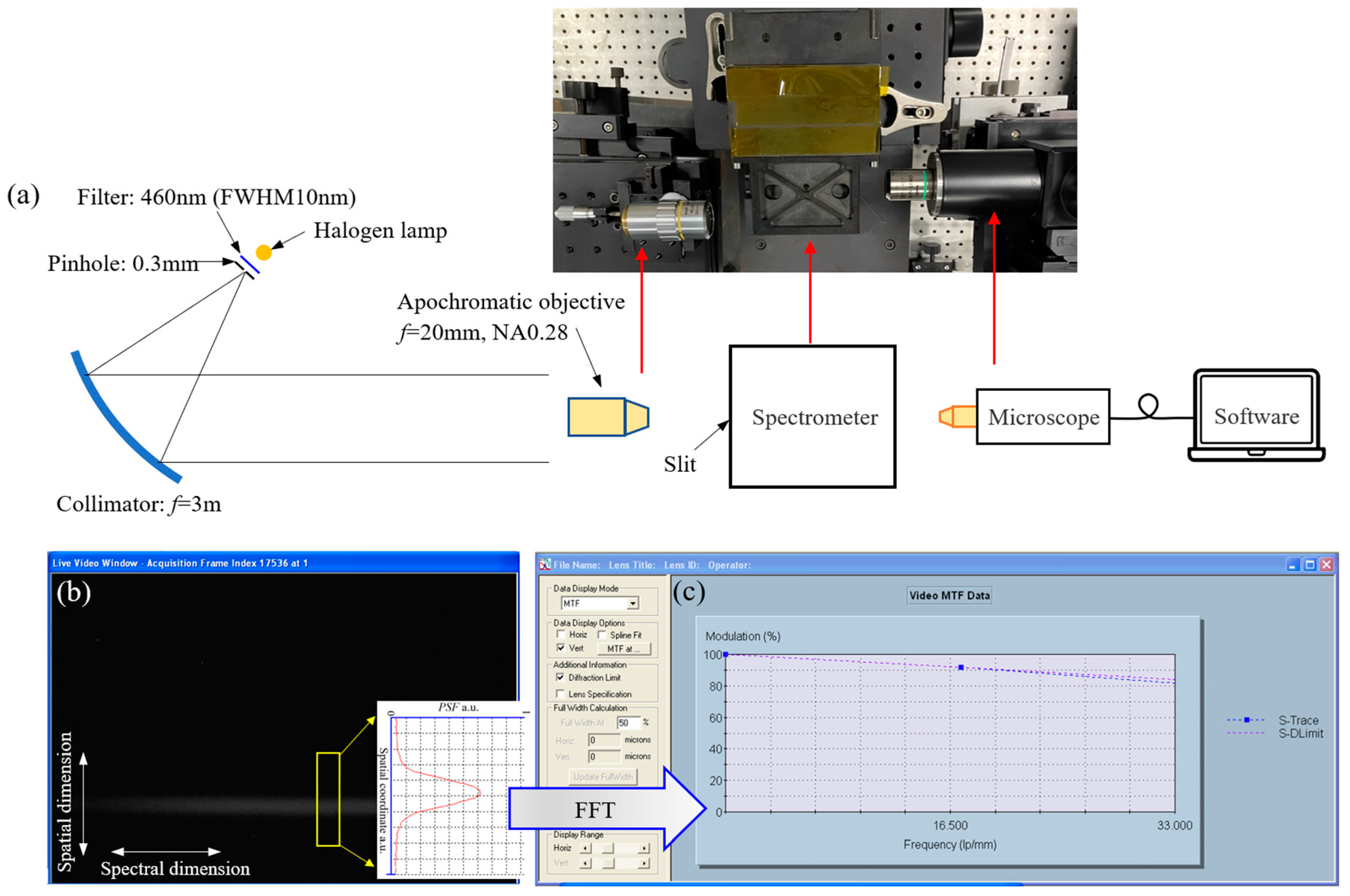
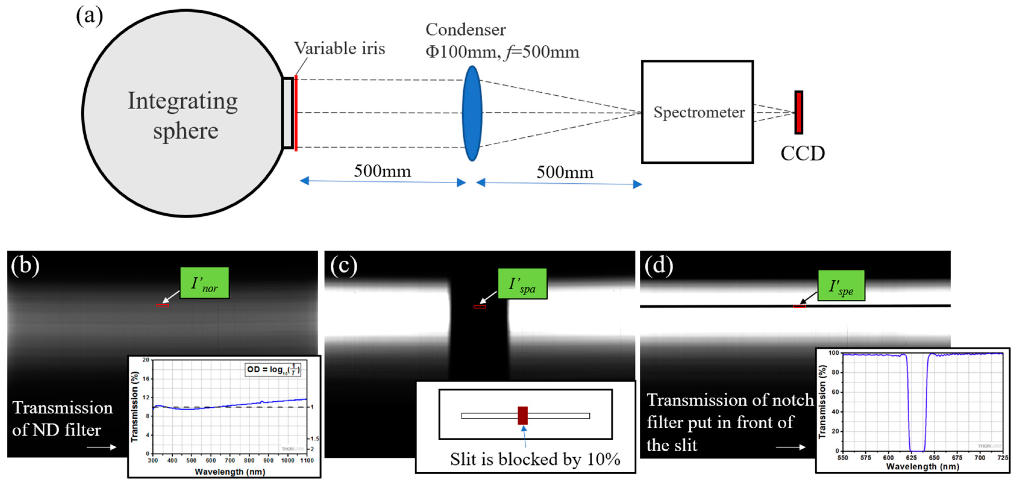
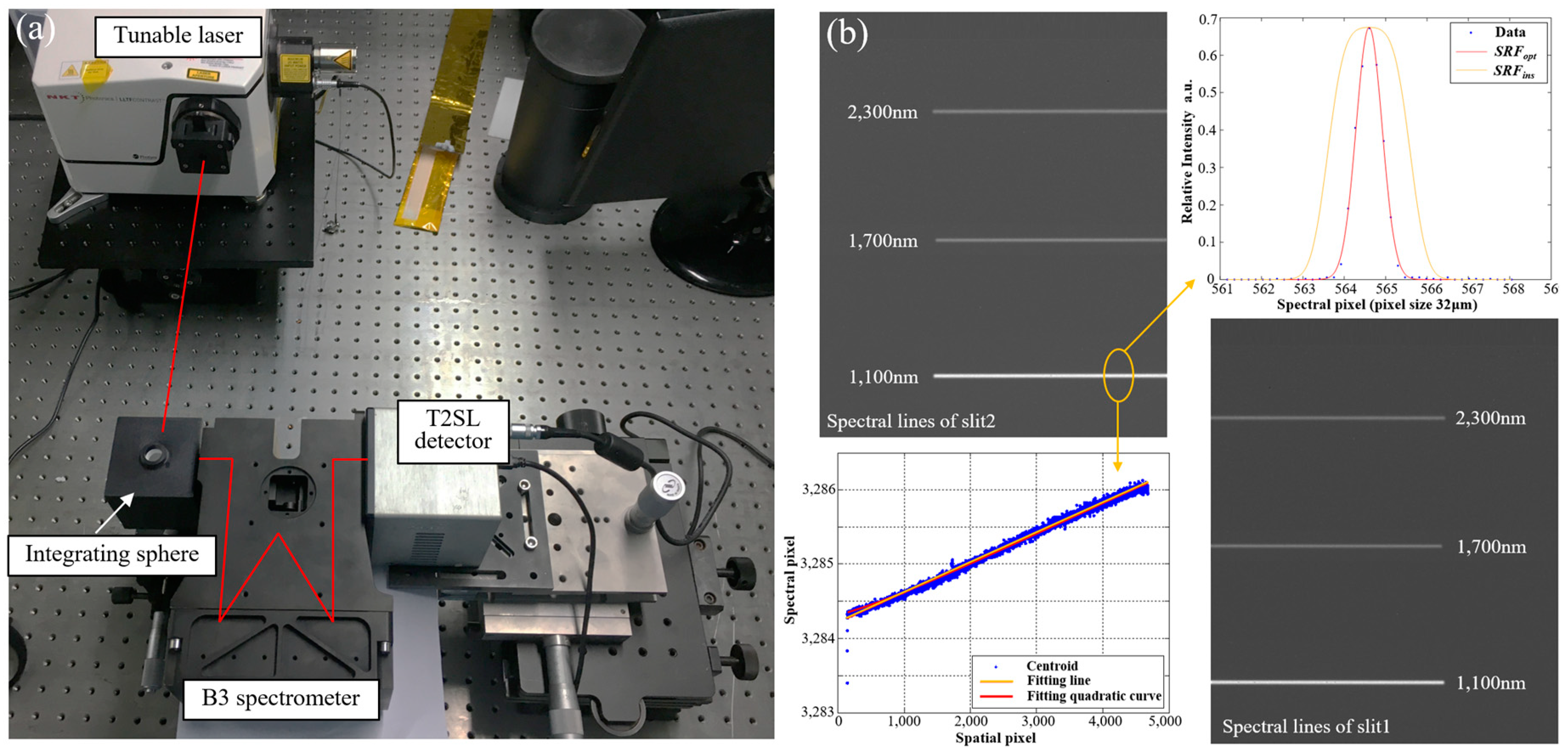
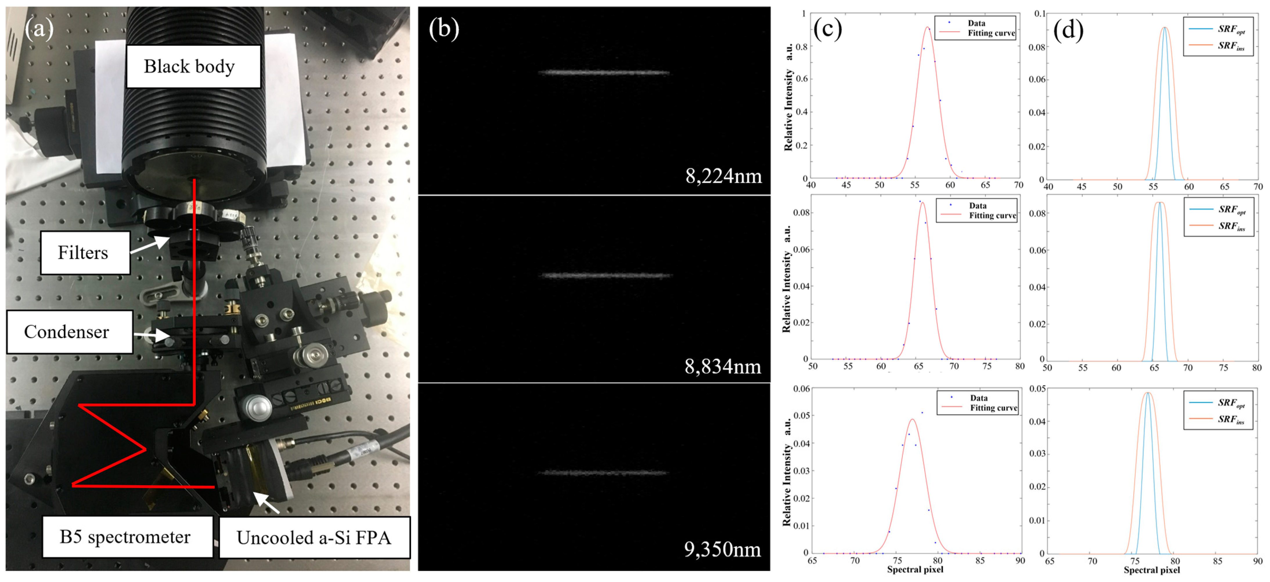
4.3. Test of Spectrometers
5. Discussion
6. Conclusions
Author Contributions
Funding
Data Availability Statement
Acknowledgments
Conflicts of Interest
References
- Vane, G.; Goetz, A.F.H.; Wellman, J.B. Airborne Imaging Spectrometer: A New Tool for Remote Sensing. IEEE Trans. Geosci. Remote Sens. 1984, GE-22, 546–549. [Google Scholar] [CrossRef]
- Green, R.O.; Eastwood, M.L.; Sarture, C.M.; Chrien, T.G.; Aronsson, M.; Chippendale, B.J.; Faust, J.A.; Pavri, B.E.; Chovit, C.J.; Solis, M.; et al. Imaging Spectroscopy and the Airborne Visible/Infrared Imaging Spectrometer (AVIRIS). Remote Sens. Environ. 1998, 65, 227–248. [Google Scholar] [CrossRef]
- Lucey, P.G.; Horton, K.A.; Williams, T.J.; Hinck, K.; Budney, C.; Rafert, B.; Rusk, T.B. SMIFTS: A cryogenically cooled, spatially modulated imaging infrared interferometer spectrometer. Proc. SPIE 1993, 1937, 130–141. [Google Scholar]
- Hall, J.L.; Boucher, R.H.; Buckland, K.N.; Gutierrez, D.J.; Hackwell, J.A.; Johnson, B.R.; Keim, E.R.; Moreno, N.M.; Ramsey, M.S.; Sivjee, M.G.; et al. MAGI: A New High-Performance Airborne Thermal-Infrared Imaging Spectrometer for Earth Science Applications. IEEE Trans. Geosci. Remote Sens. 2015, 53, 5447–5457. [Google Scholar] [CrossRef]
- Warren, D.W.; Boucher, R.H.; Gutierrez, D.J.; Keim, E.R.; Sivjee, M.G. MAKO: A high-performance, airborne imaging spectrometer for the long-wave infrared. Proc. SPIE 2010, 7812, 78120N. [Google Scholar]
- Mouroulis, P.; Van Gorp, B.; Green, R.O.; Dierssen, H.; Wilson, D.W.; Eastwood, M.; Boardman, J.; Gao, B.C.; Cohen, D.; Franklin, B.; et al. Portable Remote Imaging Spectrometer Coastal Ocean Sensor: Design, Characteristics, and First Flight Results. Appl. Opt. 2014, 53, 1363–1380. [Google Scholar] [CrossRef] [Green Version]
- Pearlman, J.S.; Carman, S.L.; Segal, C.C.; Jarecke, P.; Clancy, P.; Browne, W. Overview of the Hyperion Imaging Spectrometer for the NASA EO-1 Mission. In Proceedings of the IGARSS 2001, Scanning the Present and Resolving the Future, IEEE 2001 International Geoscience and Remote Sensing Symposium, Sydney, NSW, Australia, 9–13 July 2001. [Google Scholar]
- Pearlman, J.S.; Barry, P.S.; Segal, C.C.; Shepanski, J.; Beiso, D.; Carman, S.L. Hyperion, a Space-Based Imaging Spectrometer. IEEE Trans. Geosci. Remote Sens. 2003, 41, 1160–1173. [Google Scholar] [CrossRef]
- Rast, M.; Bezy, J.L.; Bruzzi, S. The ESA Medium Resolution Imaging Spectrometer MERIS a Review of the Instrument and Its Mission. Int. J. Remote Sens. 1999, 20, 1681–1702. [Google Scholar]
- Nieke, J.; Borde, F.; Mavrocordatos, C.; Berruti, B.; Delclaud, Y.; Riti, J.B.; Garnier, T. The ocean and land colour imager (OLCI) for the Sentinel 3 GMES mission: Status and first test results. Proc. SPIE 2012, 8528, 85280C. [Google Scholar]
- Lucke, R.L.; Corson, M.; McGlothlin, N.R.; Butcher, S.D.; Wood, D.L.; Korwan, D.R.; Li, R.R.; Snyder, W.A.; Davis, C.O.; Chen, D.T. Hyperspectral Imager for the Coastal Ocean: Instrument Description and First Images. Appl. Opt. 2011, 50, 1501–1516. [Google Scholar] [CrossRef]
- Pan, Q.; Chen, X.; Zhou, J.; Liu, Q.; Zhao, Z.; Shen, W. Manufacture of the Compact Conical Diffraction Offner Hyperspectral Imaging Spectrometer. Appl. Opt. 2019, 58, 7298–7304. [Google Scholar] [CrossRef] [PubMed]
- Guanter, L.; Kaufmann, H.; Segl, K.; Foerster, S.; Rogass, C.; Chabrillat, S.; Kuester, T.; Hollstein, A.; Rossner, G.; Chlebek, C.; et al. The EnMAP Spaceborne Imaging Spectroscopy Mission for Earth Observation. Remote Sens. 2015, 7, 8830–8857. [Google Scholar] [CrossRef] [Green Version]
- Peschel, T.; Beier, M.; Damm, C.; Hartung, J.; Jende, R.; Müller, S.; Rohde, M.; Gebhardt, A.; Risse, S.; Walter, I.; et al. Integration and testing of an imaging spectrometer for earth observation. Proc. SPIE 2018, 11180, 111800O-2. [Google Scholar]
- Mouroulis, P.; Green, R.O.; Van, G.B.; Moore, L.B.; Wilson, D.W.; Bender, H.A. Landsat Swath Imaging Spectrometer Design. Opt. Eng 2016, 55, 015104. [Google Scholar] [CrossRef]
- Cogliati, S.; Sarti, F.; Chiarantini, L.; Cosi, M.; Lorusso, R.; Lopinto, E.; Miglietta, F.; Genesio, L.; Guanter, L.; Damm, A.; et al. The PRISMA Imaging Spectroscopy Mission: Overview and First Performance Analysis. Remote Sens. Environ. 2021, 262, 112499. [Google Scholar] [CrossRef]
- Lockwood, R.B.; Cooley, T.W.; Nadile, R.M.; Gardner, J.A.; Armstrong, P.S.; Payton, A.M.; Davis, T.M.; Straight, S.D. Advanced responsive tactically effective military imaging spectrometer (ARTEMIS): System overview and objectives. Proc. SPIE 2007, 6661, 666102. [Google Scholar]
- Zeng, C.; Han, Y.; Liu, B.; Sun, P.; Li, X.; Chen, P. Optical Design of a High-Resolution Spectrometer with a Wide Field of View. Opt. Lasers Eng. 2021, 140, 106547. [Google Scholar] [CrossRef]
- Dwight, J.G.; Tkaczyk, T.S.; Alexander, D.; Pawlowski, M.E.; Stoian, R.-I.; Luvall, J.C.; Tatum, P.F.; Jedlovec, G.J. Compact Snapshot Image Mapping Spectrometer for Unmanned Aerial Vehicle Hyperspectral Imaging. J. Appl. Rem. Sens. 2018, 12, 044004. [Google Scholar] [CrossRef]
- Mu, T.; Han, F.; Li, H.; Tuniyazi, A.; Li, Q.; Gong, H.; Wang, W.; Liang, R. Snapshot Hyperspectral Imaging Polarimetry with Full Spectropolarimetric Resolution. Opt. Lasers Eng. 2022, 148, 106767. [Google Scholar] [CrossRef]
- Bourdarot, G.; Le Coarer, E.; Bonfils, X.; Alecian, E.; Rabou, P.; Magnard, Y. NanoVipa: A Miniaturized High-Resolution Echelle Spectrometer, for the Monitoring of Young Stars from a 6U Cubesat. CEAS Space J. 2017, 9, 411–419. [Google Scholar] [CrossRef]
- Zhu, J.; Shen, W. Analytical Design of Athermal Ultra-Compact Concentric Catadioptric Imaging Spectrometer. Opt. Express 2019, 27, 31094–31109. [Google Scholar] [CrossRef] [PubMed]
- Chrisp, M.P.; Lockwood, R.B.; Smith, M.A.; Balonek, G.; Holtsberg, C.; Thome, K.J.; Murray, K.E.; Ghuman, P. Development of a Compact Imaging Spectrometer Form for the Solar Reflective Spectral Region. Appl. Opt. 2020, 59, 10007. [Google Scholar] [CrossRef] [PubMed]
- Cook, L.G.; Silny, J.F. Imaging spectrometer trade studies: A detailed comparison of the Offner-Chrisp and reflective triplet optical design forms. Proc. SPIE 2010, 7813, 78130F. [Google Scholar]
- Yuan, L.; He, Z.; Lv, G.; Wang, Y.; Li, C.; Xie, J.; Wang, J. Optical design, laboratory test, and calibration of airborne long wave infrared imaging spectrometer. Opt. Express 2017, 25, 22440–22454. [Google Scholar] [CrossRef] [PubMed]
- Krimchansky, A.; Machi, D.; Cauffman, S.A.; Davis, M.A. Next-generation geostationary operational environmental satellite (GOES-R series): A space segment overview. Proc. SPIE 2004, 5570, 155–164. [Google Scholar]
- Aminou, D.M.A.; Jacquet, B.; Pasternak, F. Characteristics of the meteosat second generation (MSG) radiometer/imager: SEVIRI. Proc. SPIE 1997, 3221, 19–31. [Google Scholar]
- Vaillon, L.; Schull, U.; Knigge, T.; Bevillon, C. Geo-Oculus: High resolution multi-spectral Earth imaging mission from geostationary orbit. Proc. SPIE 2010, 10565, 105651V-2. [Google Scholar]
- Elwell, J.D.; Cantwell, G.W.; Scott, D.K.; Esplin, R.W.; Hansen, G.B.; Jensen, S.M.; Jensen, M.D.; Brown, S.B.; Zollinger, L.J.; Thurgood, V.A.; et al. A Geosynchronous Imaging Fourier Transform Spectrometer (GIFTS) for Hyperspectral Atmospheric Remote Sensing: Instrument Overview and Preliminary Performance Results. Proc. SPIE 2006, 6297, 62970S. [Google Scholar]
- Tufillaro, N.; Davis, C.O.; Valle, T.; Good, W.; Stephens, M.; Spuhle, R.P. Behavioral Model and Simulator for the Multi-Slit Optimized Spectrometer (MOS). Proc. SPIE 2013, 8870, 88700E-1. [Google Scholar]
- Butz, A.; Orphal, J.; Checa-Garcia, R.; Friedl-Vallon, F.; von Clarmann, T.; Bovensmann, H.; Hasekamp, O.; Landgraf, J.; Knigge, T.; Weise, D.; et al. Geostationary Emission Explorer for Europe (G3E): Mission Concept and Initial Performance Assessment. Atmos. Meas. Technol. 2015, 8, 4719–4734. [Google Scholar] [CrossRef] [Green Version]
- Choi, W.J.; Moon, K.J.; Yoon, J.; Cho, A.; Kim, S.; Lee, S.; Ko, D.H.; Kim, J.; Ahn, M.H.; Kim, D.R.; et al. Introducing the Geostationary Environment Monitoring Spectrometer. J. Appl. Rem. Sens. 2018, 12, 0044005. [Google Scholar] [CrossRef]
- Polonsky, I.N.; O’Brien, D.M.; Kumer, J.B.; O’Dell, C.W.; the geoCARB Team. Performance of a geostationary mission, geoCARB, to measure CO2, CH4 and CO column-averaged concentrations. Atmos. Meas. Technol. 2014, 7, 959–981. [Google Scholar] [CrossRef]
- Kolm, M.G.; Maurer, R.; Sallusti, M.; Bagnasco, G.; Gulde, S.T.; Smith, D.J.; Bazalgette, C.G. Sentinel 4: A geostationary imaging UVN spectrometer for air quality monitoring: Status of design, performance and development. Proc. SPIE 2014, 10563, 1056341. [Google Scholar]
- Zoogman, P.; Liu, X.; Suleiman, R.M.; Pennington, W.F.; Flittner, D.E.; Al-Saadi, J.A.; Hilton, B.B.; Nicks, D.K.; Newchurch, M.J.; Carr, J.L.; et al. Tropospheric Emissions: Monitoring of Pollution (TEMPO). J. Quant. Spectrosc. Radiat. Transf. 2017, 186, 17–39. [Google Scholar] [CrossRef] [Green Version]
- Lu, F.; Shou, Y. Channel Simulation for FY-4 AGRI. In Proceedings of the 2011 IEEE International Geoscience and Remote Sensing Symposium, Vancouver, BC, Canada, 24–29 July 2011; pp. 3265–3268. [Google Scholar]
- Liu, Y.N.; Sun, D.X.; Hu, X.N.; Ye, X.; Li, Y.D.; Liu, S.F.; Cao, K.Q.; Chai, M.Y.; Zhou, W.Y.N.; Zhang, J.; et al. The Advanced Hyperspectral Imager: Aboard China’s GaoFen-5 Satellite. IEEE Geosci. Remote Sens. Mag. 2019, 7, 23–32. [Google Scholar] [CrossRef]
- Li, Q.; Han, L.; Jin, Y.M.; Shen, W.M. Afocal three-mirror anastigmat with zigzag optical axis for widened field of view and enlarged aperture. Proc. SPIE 2016, 9618, 96180D. [Google Scholar]
- Mouroulis, P.; McKerns, M.M. Pushbroom Imaging Spectrometer with High Spectroscopic Data Fidelity: Experimental Demonstration. Opt. Eng 2000, 39, 808–816. [Google Scholar] [CrossRef]
- Mouroulis, P.; Green, R.O. Review of High Fidelity Imaging Spectrometer Design for Remote Sensing. Opt. Eng. 2018, 57, 040901. [Google Scholar] [CrossRef] [Green Version]
- Kwo, D.; Lawrence, G.; Chrisp, M. Design of a grating spectrometer from a 1:1 Offner mirror system. Proc. SPIE 1987, 818, 275–279. [Google Scholar]
- Prieto-Blanco, X.; de la Fuente, R. Compact Offner–Wynne Imaging Spectrometers. Opt. Commun. 2014, 328, 143–150. [Google Scholar] [CrossRef]
- Zhu, J.; Shen, W. Design and Manufacture of Compact Long-Slit Spectrometer for Hyperspectral Remote Sensing. Optik 2021, 247, 167896. [Google Scholar] [CrossRef]
- Reimers, J.; Bauer, A.; Thompson, K.P.; Rolland, J.P. Freeform Spectrometer Enabling Increased Compactness. Light Sci. Appl. 2017, 6, e17026. [Google Scholar] [CrossRef]
- Zhu, J.; Chen, X.; Zhao, Z.; Shen, W. Design and Manufacture of Miniaturized Immersed Imaging Spectrometer for Remote Sensing. Opt. Express 2021, 29, 22603–22613. [Google Scholar] [CrossRef] [PubMed]
- Montero-Orille, C.; Prieto-Blanco, X.; González-Núñez, H.; de la Fuente, R. Design of Dyson Imaging Spectrometers Based on the Rowland Circle Concept. Appl. Opt. 2011, 50, 6487–6494. [Google Scholar] [CrossRef] [PubMed]
- Van, G.B.; Mouroulis, P.; Wilson, D.W.; Green, R.O. Design of the compact wide swath imaging spectrometer (CWIS). Proc. SPIE 2014, 9222, 92220C. [Google Scholar]
- Chrisp, M.P. Imaging Spectrometer Wide Field Catadioptric Design. US Patent 7414719B, 19 August 2008. [Google Scholar]
- Prieto-Blanco, X.; Montero-Orille, C.; Couce, B.; de la Fuente, R. Analytical Design of an Offner Imaging Spectrometer. Opt. Express 2006, 14, 9156–9168. [Google Scholar] [CrossRef]
- Zhu, J.; Chen, X.; Zhao, Z.; Shen, W. Long-Slit Polarization-Insensitive Imaging Spectrometer for Wide-Swath Hyperspectral Remote Sensing from a Geostationary Orbit. Opt. Express 2021, 29, 26851–26864. [Google Scholar] [CrossRef]
- Reimers, J.; Thompson, K.; Whiteaker, K.L.; Rolland, J.P. Spectral full-field displays for spectrometers. Proc. SPIE 2014, 9293, 92930O. [Google Scholar]
- Cobb, J.M.; Comstock, L.E.; Dewa, P.G.; Dunn, M.M.; Flint, S.D. Innovative manufacturing and test technologies for imaging hyperspectral spectrometers. Proc. SPIE 2006, 6233, 62330R. [Google Scholar]
- Beier, M.; Hartung, J.; Peschel, T.; Damm, C.; Gebhardt, A.; Scheiding, S.; Stumpf, D.; Zeitner, U.D.; Risse, S.; Eberhardt, R.; et al. Development, Fabrication, and Testing of an Anamorphic Imaging Snap-Together Freeform Telescope. Appl. Opt. 2015, 54, 3530–3542. [Google Scholar] [CrossRef]


| Specifications and Parameters | Values | ||||
|---|---|---|---|---|---|
| Orbital altitude | geostationary orbit (~36,000 km) | ||||
| Swath width/km | 400 × 400 | ||||
| FOV | 0.64° × 0.64° | ||||
| Entrance pupil diameter/m | 3.2 | ||||
| Band | B1 (UVIS) | B2 (VNIR) | B3 (SWIR) | B4 (MWIR) | B5 (LWIR) |
| Wavelength range/μm | 0.3–0.56 | 0.55–1.01 | 1–2.5 | 3–5 | 8–12.5 |
| Spatial resolution/m | 25 | 25 | 50 | 50 | 100 |
| Spectral resolution (FWHM)/nm | 4 | 5 | 12 | 50 | 200 |
| Spectral sampling distance/nm | 4 | 5 | 12 | 50 | 200 |
| MTF | 0.17 | 0.17 | 0.17 | 0.12 | 0.12 |
| Focal length/m | 21.6 | 21.6 | 17.28 | 17.28 | 8.64 |
| F number | 6.75 | 6.75 | 5.4 | 5.4 | 2.7 |
| Detector resolution | 4096 × 2048 | 4096 × 2048 | 2048 × 256 | 2048 × 256 | 1024 × 256 |
| Pixel size/μm | 15 × 15 | 15 × 15 | 24 × 32 | 24 × 32 | 24 × 32 |
| Pixels per spectral channel | 6 | 6 | 2 | 3 | 3 |
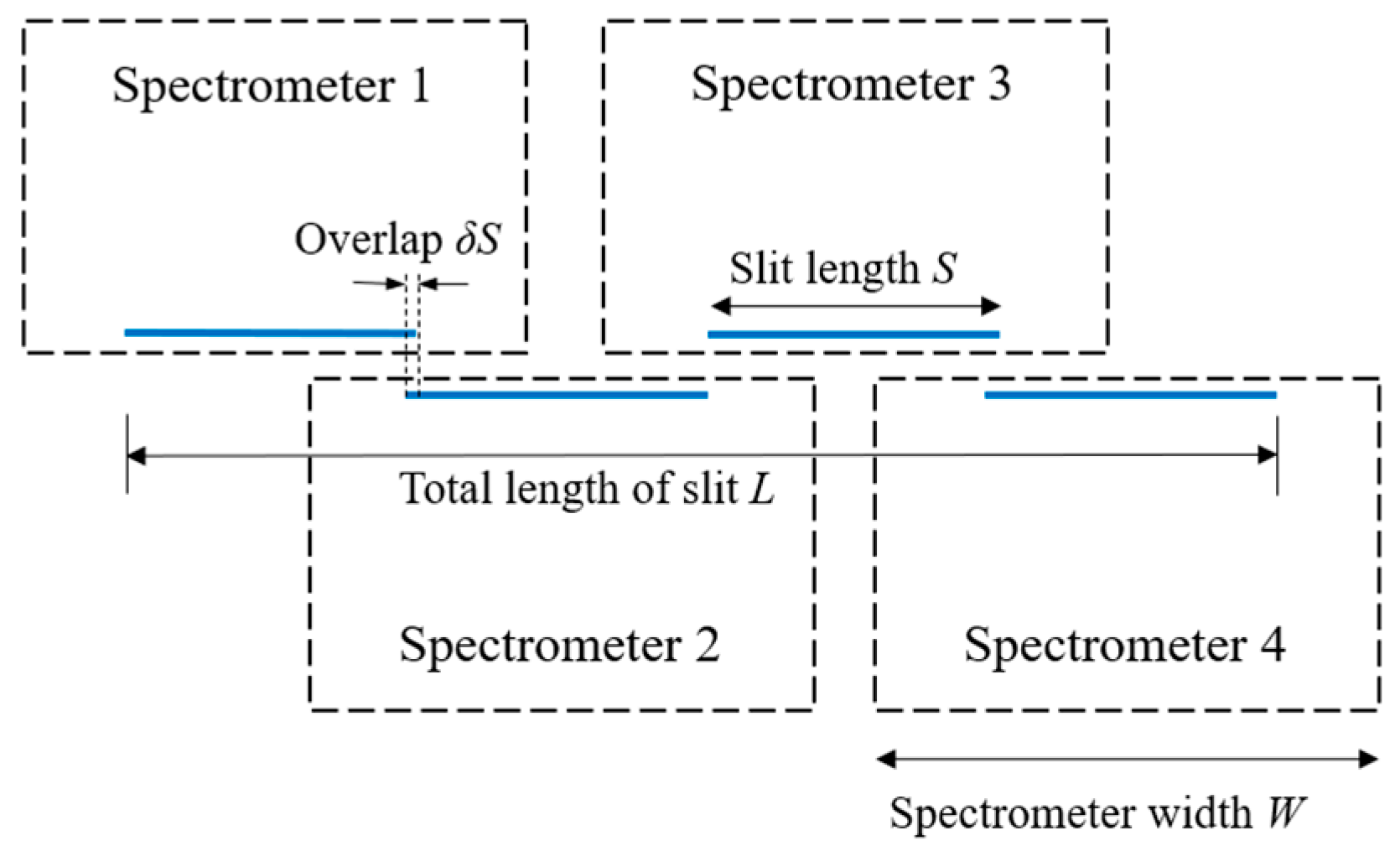
| Total length of slit/mm | 241.3 | 241.3 | 193 | 193 | 96.5 |
| Number of splicing spectrometers | 4 | 4 | 4 | 4 | 4 |
| Single slit length/mm | 61.44 | 61.44 | 49.152 | 49.152 | 24.576 |
| Slit width/μm | 15 | 15 | 24 | 24 | 24 |
| GEO | LEO | |||||
|---|---|---|---|---|---|---|
| Specifications | GeoFWHIS | GOES-R ABI [26] | FY-4 AGRI [36] | EO-1 Hyperion [8] | GF-5 AHSI [37] | EnMAP HIS [13] |
| Orbital altitude/km | 36,000 | 36,000 | 36,000 | 705 | 705 | 650 |
| Swath width/km | 400 | 1000 | 1000 | 7.5 | 60 | 30 |
| Wavelength range/μm | 0.3–12.5 | 0.45–13.6 | 0.45–13.8 | 0.4–2.5 | 0.4–2.5 | 0.42–2.45 |
| Spatial resolution/m | 25–100 | 500–2000 | 500–4000 | 30 | 30 | 30 |
| Spectral resolution/nm | 4–200 | 15–1000 | 30–1000 | 10 | 5–10 | 5.5–11.5 |
| Spectral channels | 350 | 16 | 14 | 220 | 330 | 228 |
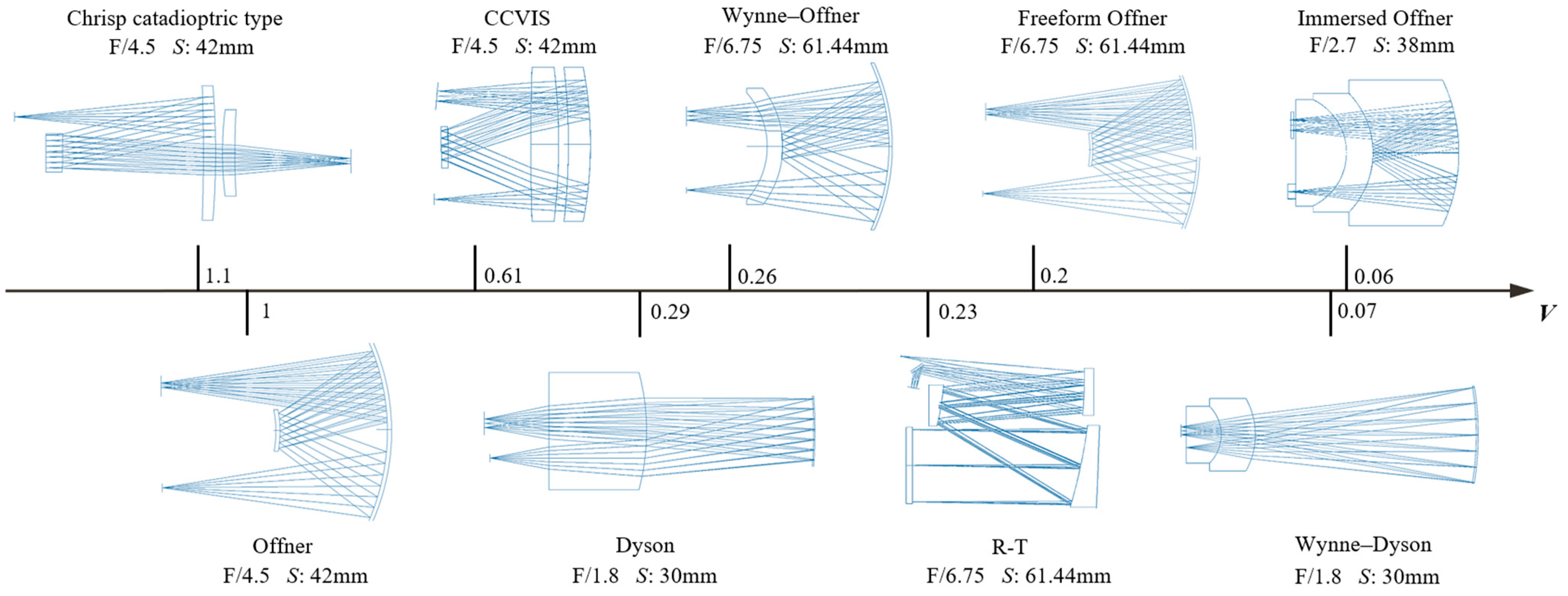
| Spectrometer Types | WFE /λ | Smile /μm | Keystone /μm | V | Characteristics |
|---|---|---|---|---|---|
| Offner | 0.10 | 0.12 | 0.09 | 1 |
|
| Wynne–Offner | 0.04 | 0.02 | 0.07 | 0.26 |
|
| Freeform Offner | 0.07 | 0.08 | 0.15 | 0.2 |
|
| Immersed Offner | 0.03 | 0.03 | 0.08 | 0.06 |
|
| Dyson | 0.18 | 0.35 | 0.22 | 0.29 |
|
| Wynne–Dyson | 0.06 | 0.12 | 0.10 | 0.07 |
|
| R-T | 0.09 | 1.55 | 1.03 | 0.23 |
|
| Chrisp catadioptric type | 0.24 | 2.20 | 2.35 | 1.1 |
|
| CCVIS | 0.11 | 0.34 | 0.25 | 0.61 |
|
| Bands | B1 | B2 | B3 | B4 | B5 |
|---|---|---|---|---|---|
| MTF | 0.86 | 0.77 | 0.72 | 0.41 | 0.28 |
| Smile/pixel | 0.06% | 0.11% | 0.26% | 0.31% | 0.95% |
| Keystone/pixel | 0.33% | 0.47% | 0.79% | 0.42% | 1.00% |
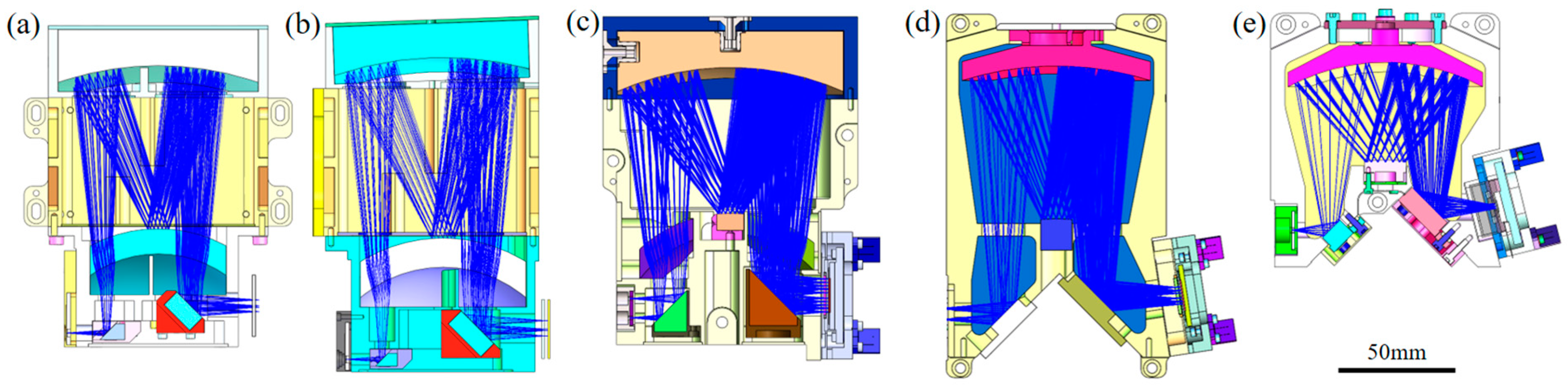
| Size/mm | 140 × 110 × 100 | 170 × 111 × 106 | 160 × 132 × 89 | 168 × 165 × 88 | 90 × 92 × 49 |
| Wavelength/nm | FWHM of SRF at Different Fields/nm | |||||
|---|---|---|---|---|---|---|
| −1 Field | −0.5 Field | 0 Field | +0.5 Field | +1 Field | Average | |
| 312.9 | 3.92 | 3.93 | 3.93 | 3.92 | 3.93 | 3.95 |
| 346.3 | 3.98 | 3.97 | 3.95 | 3.97 | 3.96 | 3.98 |
| 404.6 | 4.02 | 3.98 | 3.99 | 4.00 | 4.00 | 4.01 |
| 435.8 | 4.01 | 4.02 | 4.01 | 4.00 | 4.02 | 4.02 |
| 467.8 | 3.99 | 3.98 | 3.98 | 3.98 | 4.00 | 4.00 |
| 479.9 | 4.02 | 4.01 | 4.01 | 4.00 | 4.02 | 4.02 |
| 508.5 | 4.01 | 4.02 | 4.01 | 4.00 | 4.01 | 4.01 |
| 546.1 | 4.01 | 4.02 | 4.00 | 3.99 | 4.00 | 4.00 |
| Wavelength/nm | FWHM of SRF at Different Slits/nm | |
|---|---|---|
| Slit 1 | Slit 2 | |
| 1100 | 12.1 | 12.1 |
| 1400 | 12.0 | 12.0 |
| 1700 | 11.9 | 11.9 |
| 2000 | 12.0 | 11.9 |
| 2300 | 12.2 | 12.1 |
| Wavelength/nm | FWHM of SRF at Different Fields/nm | |||
|---|---|---|---|---|
| −1 Field | 0 Field | +1 Field | Average | |
| 8224 | 201.3 | 201.0 | 200.9 | 201.1 |
| 8834 | 202.4 | 202.1 | 201.9 | 202.1 |
| 9350 | 205.9 | 204.9 | 204.2 | 205.0 |
Disclaimer/Publisher’s Note: The statements, opinions and data contained in all publications are solely those of the individual author(s) and contributor(s) and not of MDPI and/or the editor(s). MDPI and/or the editor(s) disclaim responsibility for any injury to people or property resulting from any ideas, methods, instructions or products referred to in the content. |
© 2023 by the authors. Licensee MDPI, Basel, Switzerland. This article is an open access article distributed under the terms and conditions of the Creative Commons Attribution (CC BY) license (https://creativecommons.org/licenses/by/4.0/).
Share and Cite
Zhu, J.; Zhao, Z.; Liu, Q.; Chen, X.; Li, H.; Tang, S.; Shen, W. Geostationary Full-Spectrum Wide-Swath High-Fidelity Imaging Spectrometer: Optical Design and Prototype Development. Remote Sens. 2023, 15, 396. https://doi.org/10.3390/rs15020396
Zhu J, Zhao Z, Liu Q, Chen X, Li H, Tang S, Shen W. Geostationary Full-Spectrum Wide-Swath High-Fidelity Imaging Spectrometer: Optical Design and Prototype Development. Remote Sensing. 2023; 15(2):396. https://doi.org/10.3390/rs15020396
Chicago/Turabian StyleZhu, Jiacheng, Zhicheng Zhao, Quan Liu, Xinhua Chen, Huan Li, Shaofan Tang, and Weimin Shen. 2023. "Geostationary Full-Spectrum Wide-Swath High-Fidelity Imaging Spectrometer: Optical Design and Prototype Development" Remote Sensing 15, no. 2: 396. https://doi.org/10.3390/rs15020396