Article

A Spatial Cross-Scale Attention Network and Global Average Accuracy Loss for SAR Ship Detection

1
School of Electronical and Information Engineering, Shenyang Aerospace University, Shenyang 110136, China
2
School of Integrated Circuits, Tsinghua University, Beijing 100084, China
*
Author to whom correspondence should be addressed.
Remote Sens. 2023, 15(2), 350; https://doi.org/10.3390/rs15020350
Submission received: 11 November 2022 / Revised: 31 December 2022 / Accepted: 3 January 2023 / Published: 6 January 2023

Abstract

:
A neural network-based object detection algorithm has the advantages of high accuracy and end-to-end processing, and it has been widely used in synthetic aperture radar (SAR) ship detection. However, the multi-scale variation of ship targets, the complex background of near-shore scenes, and the dense arrangement of some ships make it difficult to improve detection accuracy. To solve the above problem, in this paper, a spatial cross-scale attention network (SCSA-Net) for SAR image ship detection is proposed, which includes a novel spatial cross-scale attention (SCSA) module for eliminating the interference of land background. The SCSA module uses the features at each scale output from the backbone to calculate where the network needs attention in space and enhances the features of the feature pyramid network (FPN) output to eliminate interference from noise, and land complex backgrounds. In addition, this paper analyzes the reasons for the “score shift” problem caused by average precision loss (AP loss) and proposes the global average precision loss (GAP loss) to solve the “score shift” problem. GAP loss enables the network to distinguish positive samples and negative samples faster than focal loss and AP loss, and achieve higher accuracy. Finally, we validate and illustrate the effectiveness of the proposed method by performing it on SAR Ship Detection Dataset (SSDD), SAR-ship-dataset, and High-Resolution SAR Images Dataset (HRSID). The experimental results show that the proposed method can significantly reduce the interference of background noise on the ship detection results, improve the detection accuracy, and achieve superior results to the existing methods.

1. Introduction

Synthetic aperture radar (SAR) is a microwave sensor based on the scattering characteristics of electromagnetic waves for imaging, which has a certain cloud and ground penetration capability to detect hidden targets. This characteristic makes it suited for marine monitoring, mapping, and military applications. With the continuous exploitation of marine resources, the monitoring of marine vessels based on SAR images has received increasing attention. SAR image object detection aims to automatically locate and identify specific targets from images and has important application prospects in defense and civil fields such as target identification, target detection, marine development, and terrain classification [1,2,3,4].
The development of SAR image ship detection methods can be divided into two stages [5]: traditional detection methods represented by constant false alarm rate (CFAR) algorithms and deep learning methods represented by convolutional neural networks. The constant false alarm rate algorithm adaptively adjusts the threshold value using statistical models and sample selection strategies. It has been widely used due to its constant false alarm rate and low complexity. For example, the bilateral CFAR algorithm [6] takes into account the intensity distribution and spatial distribution when selecting thresholds to improve the accuracy of detection. The two-parameter CFAR [7] uses log-normal as the statistical model with more accurate parameter estimation and achieves better detection performance in a multi-target environment. The modified CFAR algorithm proposed in the paper [8] uses variable guard windows to improve its detection performance for the multi-scale scene. Li et al. [9] propose an adaptive CFAR method based on intensity and texture feature fusion attention contrast mechanism to suppress clutter background and speckle noise with better performance in complex backgrounds and multi-target marine environments. The above CFAR algorithms rely on the land-segmentation algorithm in the nearshore scene, while the adaptive superpixel-level CFAR algorithm [10] is based on the superpixel segmentation method, which does not require additional land-segmentation algorithm, and its detection performance is still reliable in near-shore scenarios. However, these algorithms are based on the modeling of clutter statistical features, which are more sensitive to the complex shoreline, ocean clutter, and coherent scattering noise, with low detection accuracy and poor generalization [5]. Currently, deep learning is the mainstream research direction due to its excellent feature extraction capability and end-to-end training process, which is gradually replacing the traditional methods.
In the field of target detection, deep learning methods based on convolutional neural networks have developed rapidly due to the translation invariance and weight-sharing properties of convolution. The existing target detection methods based on convolutional neural networks can be divided into two-stage and one-stage methods. The two-stage network first generates the proposed region in the first stage and then performs classification and correction of the proposed region in the second stage. This method has higher detection accuracy and better detection for small targets, such as region-convolutional neural network (R-CNN) [11], Fast R-CNN [12], Faster R-CNN [13], Sparse R-CNN [14], etc. The one-stage network does not need to generate proposed regions and directly outputs the classification and location results of the target. Although the accuracy of the one-stage network is generally lower than that of the two-stage network, they have higher detection speed and simple training steps, such as YOLO series [15,16,17,18,19,20,21,22], single shot detection (SSD) [23], RetinaNet [24], fully convolutional one-stage object detection (FCOS) [25], etc.
Since the release of the SAR ship detection dataset (SSDD) by Li et al. [26] in 2017, SAR image ship detection based on convolutional neural networks developed rapidly, and subsequently in, 2019 and 2020, Wang et al. [27] and Wei et al. [28] released the SAR-Ship-Dataset and High-Resolution SAR Images Dataset (HRSID), respectively. Additionally, in 2021, Zhang et al. [29] corrected the mislabeling of the initial version of the SSDD and used a standardized format, which further facilitated the development of the field. In recent years, Shi et al. [30] proposed a feature aggregation enhancement pyramid network (FAEPN) to enhance the extraction capability of the network for multi-scale targets, taking into account the quality of classification and regression when assigning positive and negative samples. Cui et al. [31] proposed a dense attention pyramid network (DAPN), which used dense connectivity in the feature pyramid network (FPN) to obtain richer semantic information about each scale and used a convolutional block attention module (CBAM) to enhance the features. Zhang et al. [32] proposed a quad-feature pyramid network (Quad-FPN) to extract complex multi-scale features, and then replaced non-maximal suppression (NMS) with soft non-maximal suppression (soft-NMS) to improve the detection of densely aligned targets. Li et al. [4] proposed an attention-guided balanced feature pyramid network (A-BFPN), which contained an enhanced refinement module (ERM) for reducing background interference and a channel attention-guided fusion network for reducing confounding effects in mixed feature maps. Different from the above-mentioned anchor-base network, Zhu et al. [33] proposed a novel anchor-free network based on FCOS for SAR image target detection, in which a deformable convolution (Dconv) and an improved residual network (IRN) were added to optimize the feature extraction capability of the network. Wu et al. [34] proposed the instance segmentation-assisted ship detection network (ISASDNet), with a global reasoning module, which achieved good performance in instance segmentation and object detection. Wang et al. [35] used intersection over union (IoU) K-means to solve the extreme aspect ratio problem and embedded a soft threshold attention module (STA) in the network to suppress the effects of noise and complex backgrounds. Tian et al. [36] employed an object characteristic-driven image enhancement (OCIE) module to enhance the variety of datasets and explored the dense feature reuse (DFR) module and receptive field expansion (RFE) module to increase the network receptive field and strengthen the transmission of information flow. Wei et al. [37] adopted a high-resolution feature pyramid network (HRFPN) to make full use of the information in the high-resolution and low-resolution features and proposed a high-resolution ship detection network (HR-SDNet) on this basis.
In order to further improve the detection accuracy of the network, in this paper, a new anchor-free spatial cross-scale attention network (SCSA-Net) is proposed, which contains a novel spatial cross-scale attention (SCSA) module that enhances features at different scales while mitigating the interference generated by complex backgrounds such as land. In addition, to solve the “score shift” problem of average accuracy loss (AP loss), this paper improves AP loss and proposes global average accuracy loss (GAP loss). Three widely used datasets are used to experimentally validate the proposed methods and confirm their effectiveness.
The main contributions of our work are as follows:
  • A novel cross-scale spatial attention module is proposed, which consists of a cross-scale attention module and a spatial attention redistribution module. The former dynamically adjusts the position of network attention by combining information from different scales. The latter redistributes spatial attention to mitigate the influence of complex backgrounds and make the ship more distinctive.
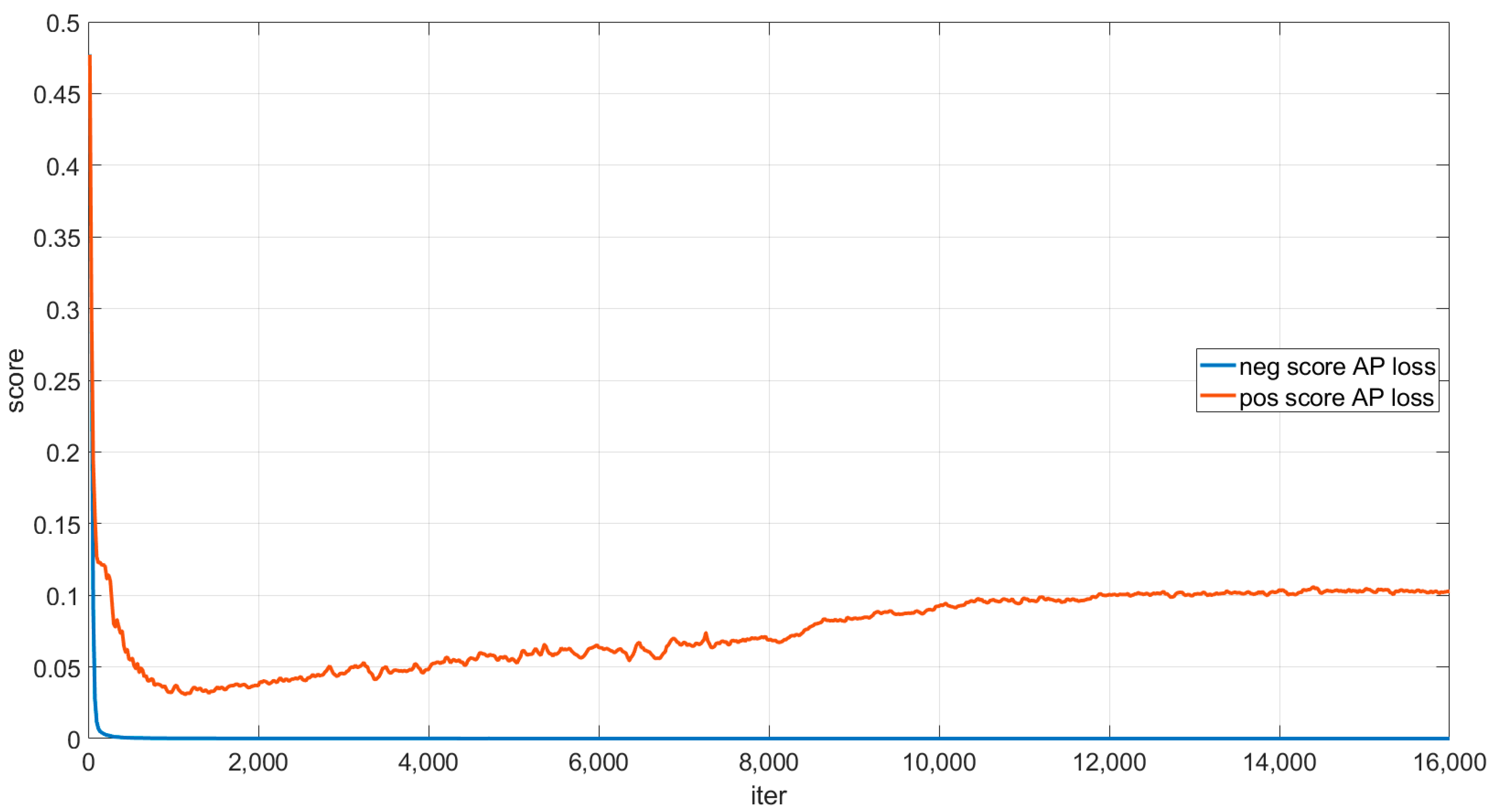
  • We analyze the reasons why AP loss generates the “score shift” problem and propose a global average accuracy loss (GAP loss) to solve it. Compared to traditional methods using focus loss as the classification loss, training with GAP loss allows the network to optimize directly with the average precision (AP) as the target and to distinguish between positive and negative samples more quickly, achieving better detection results.
  • We propose an anchor-free spatial cross-scale attention network (SCSA-Net) for ship detection in SAR images, which reached 98.7% AP on the SSDD, 97.9% AP on the SAR-Ship-Dataset and 95.4% AP on the HRSID, achieving state-of-the-art performance.
The remainder of this paper is organized as follows: the second section introduces the proposed method; the third section describes the experiments and analysis of the results; the fourth section discusses and suggests future work; finally, the fifth section summarizes this paper.

2. Methods

This section describes SCSA-Net for SAR ship detection, which contains the overall architecture of SCSA-Net, the spatial cross-scale attention module, and GAP loss.

2.1. Overall Architecture of SCSA-Net

The main framework of SCSA-Net is depicted in Figure 1. FCOS [25] is chosen as the baseline, which is one of the most representative one-stage anchor-free detectors. Following the FCOS, the ResNet-50 is used as the backbone of SCSA-Net for feature extraction and the FPN is employed to solve the multi-scale target detection problem. Additionally, a new spatial cross-scale spatial attention module is added to the network, which dynamically enhances the FPN output features based on the backbone output features. The enhanced feature is then forwarded to the class-box subnet for classification and regression.

2.2. Spatial Cross-Scale Attention Module

In the offshore scenes of SAR images, the network usually performs well because of the large distinction between sea level clutter and ship targets. However, in the near-shore scenes of SAR images, the land portion of the background is complex and the network easily confuses ship targets with smaller islands and land backgrounds having similar ship shapes. This leads to false alarms and missed detections. The spatial cross-scale attention module is proposed to reduce the interference of land-to-ship targets. It consists of two parts, the cross-scale attention module, and the spatial attention redistribution module. The cross-scale attention module determines the regions requiring attention at each scale, while the spatial attention redistribution module redistributes the attention regions at each scale spatially to locate more accurate attention regions.

2.2.1. Cross-Scale Attention Module

The structure of the cross-scale attention module is shown in Figure 2. The multi-head attention module is used to extract the attention regions of each scale more accurately. To be more intuitive, the formula in [38] is quoted as:
M u l t i H e a d Q , K , V = C o n c a t h e a d 1 , , h e a d n W O w h e r e   h e a d i = s o f t max Q W i Q K W I K T d k V W i V
where W i Q d m o d e l × d k , W i K d m o d e l × d k , W i V d m o d e l × d v , and W O d v × d m o d e l are the projection matrices, where d k and d v are the dimensions of K and V respectively, and d m o d e l is the dimension of the multi-head attention module. In this paper, the multi-head attention inputs of Q , K , and V are the same, so we simplify M u l t i H e a d Q , K , V to M u l t i H e a d X when Q = K = V = X .
The features from the last residual block of i -th stage in ResNet-50 are M i C i × H i × W i , i = 3 , 4 , 5 where Ci, Hi, Wi indicate the channel number, spatial height, and width, respectively. First, the convolution of size 1 is used in M i to obtain X i 256 × H i × W i , i = 3 , 4 , 5 in order to reduce the channel dimension. Then, the maximum pooling layer is used to downsample X i to obtain X i to reduce the computing cost X i v = V X i 256 × H 5 W 5 , i = 3 , 4 , 5 denotes the vectorization function, and X i = V 1 X i v 256 × H 5 × W 5 denotes its inverse function. The enhanced feature A i 256 × H 5 × W 5 , i = 3 , 4 , 5 are calculated as:
A i = V 1   M u l t i H e a d   V X i , i = 5 V 1   M u l t i H e a d   V X i + A i + 1 ,   i = 3 , 4

2.2.2. Spatial Attention Redistribution Module

The structure of the spatial redistribution model is shown in Figure 3. First, using a deformable convolution and concatenation on A i to obtain A c 256 3 × H 5 × W 5 . Then A c is fed into the convolution layer and SoftMax activation layer to obtain A s 5 × H 5 × W 5 . The A s j 1 × H 5 × W 5 denotes the feature map of the j -th channel in the A s , where A s j , j = 3, 4, 5 are considered as attention weights only on the j -th scale, except that some regions possibly will be interesting or suppressed at all scales, such as common features of ship targets or land areas that do not contain targets. For this reason, A s 1 and A s 2 are respectively used as the weights that require attention and suppression at all scales. Then, the redistributed attention weight S i 1 × H 5 × W 5 can be formulated as:
S i = A s i + A s 1 A s 2
Finally, S i are reshaped by upsampling into S i 1 × H i × W i used to enhance features F i , i = 3 , 4 , 5 from FPN. Following the idea of FCOS, to further improve the detection capability of large-scale targets, we use a series of convolutions of stride 2 and size 3 for the enhanced features of F 5 to obtain feature maps F 6 and F 7 with larger receptive fields.
F 6 = C o n v F 5 B D S 5
F 7 = C o n v R e L U F 6
where B D means broadcast operation, C o n v means a convolution with a kernel size of 3, a stride of 2, and a padding of 1.

2.3. Global Average Precision Loss

2.3.1. Average Precision Loss

In the object detection task, average precision (AP) is an important criterion for the detection result. The range of AP is 0 , 1 , the closer the AP is to 1, the more accurate the detection result is and the closer the AP is to 0, the worse the detection result is. The main optimization goal of the object detection task is to make the AP as close to 1 as possible. Based on this goal, AP loss was proposed by Chen et al. [39]. With a large number of samples, AP loss can achieve better performance than focal loss because it allows the network to be optimized directly for the AP, and is not affected by a large number of true negative samples [39]. To be more intuitive, the formula of AP loss in [39] is quoted as:
L A P = 1 P i P j N H s j s i 1 + j P , j i H s j s i + j N H s j s i w h e r e   H x = 0 , x < δ x 2 δ + 0.5 , δ x δ 1 , δ < x
where s i is the classification score of the box b i output by the network without the sigmoid function, and each b i will be assigned a label t i 1 , 0 , 1 (label −1 for not counted into the AP loss). P = i t i = 1 and N = i t i = 0 are the set of positive and negative samples, respectively, and P is the size of set P . Further, Chen et al. [39] give a formula for the gradient g i of s i to address the problem that L A P  is non-differentiable in the backpropagation process.
g i = j L j i y j i j L i j y i j w h e r e   L i j = H s j s i 1 + j P , j i H s j s i + j N H s j s i
where i , j , y i j = 1 t i = 1 , t j = 0 and 1 is an indicator function that equals to 1 only if the subscript condition holds (i.e., t i = 1 , t j = 0 ), otherwise 0.

2.3.2. Global Average Precision Loss

Chen et al. [39] point out that training with AP loss has the problem of “score shift”. That is, although the AP of each of the two images is high, the AP may become lower if the two images are put together, because the scores of the positive or negative samples of the two images may be in different ranges, and the score of negative samples on one of the images may be higher than the score of positive samples in the other image. Chen et al. [39] avoid this situation through minibatch training but it still exists in two different batches. The main reason for the “score shift” is that AP loss only deals with those positive samples that have smaller scores than the negative samples and those negative samples that have larger scores than the positive samples. If the score of a positive sample is larger than all the negative samples, then its gradient g i will be 0. Similarly, if the score of a negative sample is smaller than all the positive samples, then its gradient will also be 0. This leads to the fact that once the score of a sample jumps out of the range r k = max i N k s i , k , min j P k s j , k in the k -th batch, then its gradient of AP loss will become 0 unless the region changes so that it is included again, and when min j P k s j , k > max i N k s i , k , the gradient of AP loss for all samples will become 0. Thus, the greater the difference in r k , the more serious the problem of “score shift”. In addition, in the early stage of the training, the scores of positive and negative samples are very close to each other, which will result in a small range of r k . Therefore, training with AP loss can only produce a very small gap in the positive and negative samples, leading to poor results.
To solve the above problem, we propose a global average precision loss (GAP loss). First, to make the range r k of each batch similar, we calculate the mean value of positive and negative sample scores for multiple batches and take them into account separately when calculating L i j . Thus, the formula for L i j becomes as follows, while for more intuition we divide L i j into L i j P for i , j t i = 1 , t j = 0 and L i j N for i , j t i = 0 , t j = 1 .
L i j N = H s j s i 1 + j P k , j i H s j s i + j N k H s j s i + H s j s P k 1 + j P k , k i H s j s P k + j N k H s j s P k
L i j P = H s j s i + | N k | H s N k s i 1 + j P k , j i H s j s i + j N k H s j s i + | N k | H s N k s i
where P k and N k are the set of positive and negative samples in the k -th batch, respectively. P k and N k is the size of set P k and N k . s P k and s N k are the exponentially weighted averages of the positive and negative sample scores of multiple batches and are calculated as follows:
s P k = β s P k 1 + 1 β 1 P k i P k s i
s N k = β s N k 1 + 1 β 1 N k i N k s i
Compared with Equation (7), the extra term in the Equation (8) is equivalent to adding P k additional positive samples with a score of s P k to the set of positive samples. Likewise, Equation (9) adds N k additional negative samples with score s N k to the set of negative samples. In this way, the r k of each batch will contain both s N k and s P k , thus alleviating the problem of “score shift”. We then added additional terms to the gradient g i to allow the sample to still obtain a non-zero gradient even if it jumps out of r k , and the gradient of GAP loss is calculated as follows:
g i = j L j i N + L j i N γ + 1 S i g m o i d s i γ y j i j L i j P + L i j P γ + 1 1 S i g m o i d s i γ y i j
Taking positive samples as an example, positive samples with small activation values and large L i j P will obtain a larger value of g i when L i j P is not zero compared to g i , while as L i j P is equal to zero, positive samples will obtain a non-zero gradient based on their activation values, thus allowing the network to focus on those difficult positive samples with small activation values and large L i j P , while not “ignoring” those simple samples that jump out at r k .

3. Experiment

In this section, we first introduce the experimental datasets, evaluation metrics, and implementation details. Then, we conducted an ablation study to analyze SCSA-Net. Finally, we compare other recent methods with several examples.

3.1. Datasets

  • Official-SSDD (SSDD): Currently, the SSDD [26] dataset published in 2017 is the most widely used in the SAR ship detection field. Subsequently, Zhang et al. published the updated official SSDD dataset of the SSDD dataset in 2021 [29], which corrected the wrong labels in SSDD and provided richer label formats. The official SSDD dataset contains complex backgrounds and multi-scale offshore and inshore targets. Most of the images are 500 pixels wide, and the SSDD has a variety of SAR image samples with resolutions ranging from 1 m to 15 m from different sensors of RadarSat-2, Terra SAR-X, and Sentinel-1. The average size of ships in SSDD is only ~35 × 35 pixels. In this paper, we refer to Official SSDD as SSDD for convenience.
  • SAR-Ship-Dataset: SAR-Ship-Dataset was released by Wang et al. [27] in 2019. It contains 43,819 images with 256 × 256 image sizes, mainly from Sentinel-1 and Gaofen-3. SAR ships in SAR-Ship-Dataset are provided with resolutions from 5 m to 20 m, and HH, HV, VV, and VH polarizations. Same to their original reports in [27], the entire dataset is randomly divided into training (70%), validation (20%), and test dataset (10%).
  • High-Resolution SAR Images Dataset (HRSID): The HRSID proposed by Wei et al. [28] is constructed by using original SAR images from the Sentinel-1B, TerraSAR-X, and TanDEM-X satellites. The HRSID contains 5604 images of 800 × 800 size and 16,951 ship targets. These images have various polarization rates, imaging modes, imaging conditions, etc. As in its original reports in [28], the ratio of the training set and the test set is 13:7 according to its default configuration files.

3.2. Evaluation Metrics

In order to evaluate the detection performance quantitatively, the evaluation criteria we used include the precision rate, recall rate, and average precision (AP). The calculation method is as follows:
Precision = T P T P + F P
Recall = T P T P + F N
For a predicted box, if the IoU between it and the corresponding ground truth box is greater than 0.5, then it is defined as true positive ( T P ), otherwise, it is false positive ( F P ). For a ground truth box, if there is no predicted box with its IoU greater than 0.5, it is defined as a false negative ( F N ). AP is defined as:
AP = 0 1 p r d r
where p and r represents precision and recall at an IoU threshold of 0.5, and p ( ) is a function that takes r as a parameter, which is equal to taking the area under the curve.

3.3. Training Details

The ResNet-50 pre-trained on ImageNet is carried out to initialize our backbone. The initial learning rate of the SGD optimizer is 0.01, which is divided by 10 at each decay step. The number of image iterations per epoch is 16 K. All training processes are carried out on a Tesla V100 GPU (32 G) server.

3.4. Ablation Study

To visualize the effect of GAP loss, we counted the mean curves of the classification scores of positive and negative samples predicted by the network during the training phase, as shown in Figure 4, Figure 5 and Figure 6. The curves are the output of the network trained by focal loss, AP loss, and GAP loss, respectively. To be more intuitive, the classification scores are normalized by a sigmoid function to convert them into probabilities, which represents the probability that the network considers the sample to be a ship. For positive samples, it should be as close to 1 as possible, and for negative samples, it should be as close to 0 as possible. In the initial stage of training, the positive and negative sample scores of the network prediction are in the range of 0.5. No matter what kind of loss is used for training, the negative sample scores can drop to 0 quickly, but only the positive sample scores corresponding to the GAP loss can quickly increase to about 1. For the network trained with focal loss and AP loss, the output positive sample score will first drop from 0.5 to approximately 0.17 and 0.04 before gradually increasing. Additionally, since the gradient of AP loss for samples out of r k is 0, the average of the positive sample score corresponding to the AP loss at the end of training can only reach about 0.1, such that the gap of scores between positive and negative samples is relatively small, leading to poorer detection results. The focal loss can gradually increase the positive sample score of the network to about 0.9, but it is still lower than the positive sample score corresponding to the GAP loss.
To evaluate the effectiveness of the SCSA module and GAP loss, we performed ablation studies on SSDD, SAR-Ship-Dataset, and HRSID with different settings of SCSA-Net, respectively. The results of the ablation study are shown in Table 1 and Figure 7. Firstly, by adding the SCSA module, the performance of the network can be improved regardless of the loss used in training. Second, since AP loss results in a smaller gap between positive and negative sample scores, replacing the focal loss with AP loss results in a decrease in AP, with or without the SCSA module. In contrast, direct replacement of focal loss with GAP loss can improve AP with or without the SCSA module. Finally, using both the GAP loss and SCSA modules achieved the best results on all three datasets, 98.7% AP on the SSDD dataset, 97.9% AP on the SAR-Ship-Dataset dataset, and 95.4% AP on the HRSID dataset, respectively.
Some visualization results of the ablation experiments on SSDD, SAR-Ship-Dataset, and HRSID are shown in Figure 8, Figure 9 and Figure 10, where Figure 8a–d–Figure 10a–d show the ground truths, detection results of FCOS trained by focal loss, detection results of FCOS trained by GAP loss, and detection results of FCOS with SCSA module trained by GAP loss, respectively. The samples include different background states in the offshore, deep sea, and moored in port, respectively. Since some of the ships have large noise and more complex nearshore backgrounds, the detection results of FCOS are easily affected by them, leading to missed detections and false alarms, as shown in Figure 8, Figure 9 and Figure 10b. By training FCOS with GAP loss, the scores of negative samples can be effectively reduced and the scores of positive samples can be increased, resulting in better AP, as shown in Figure 8, Figure 9 and Figure 10c. However, for some difficult samples, even training with GAP loss still cannot achieve good results due to the limited expressiveness of the network. By adding the SCSA module, the feature extraction capability of the network is improved, and the problem of missed detection and false alarm in some near-shore scenes is effectively solved, as shown in Figure 8, Figure 9 and Figure 10d.
To further confirm the effectiveness of the SCSA module, we use different configurations of the SCSA module in the network and train the network using GAP loss. The detection results on SSDD, SAR-Ship-Dataset, and HRSID are shown in Table 2. The difference in settings is whether A s 1 and A s 2 are considered when calculating S i in the Equation (3). The AP values of the results can be improved by using either A s 1 or A s 2 on the three different datasets. By using A s 1 additionally in the calculation of S i , 0.096%, 0.187%, and 0.157% AP are improved on the SSDD, SAR-Ship-Dataset, and HRSID, respectively. By using A s 2 in the calculation of S i , 0.116%, 0.195%, and 0.184% AP are improved on the SSDD, SAR-Ship-Dataset, and HRSID, respectively. Additionally, the best detection results can be achieved by using A s 1 and A s 2 together, with an improvement of 0.270%, 0.311%, and 0.346% AP on the SSDD, SAR-Ship-Dataset, and HRSID, respectively.

3.5. Comparison with the Latest SAR Ship Detection Methods

To further demonstrate the advancement and superiority of our proposed method, we experimentally validated with the latest SAR ship detection method using the SSDD, SAR-Ship-Dataset, and HRSID, as shown in Table 3, Table 4 and Table 5. The proposed method achieves the best results on all three widely used datasets. On the SSDD, ISASDNet+r101 [34] achieves the highest 96.8% AP in the two-stage network, while the proposed SCSA-Net can achieve 98.7% AP, which is 1.9% AP improvement compared to ISASDNet+r101 [34] and 0.3% AP improvement compared to the anchor-free network proposed by Zhu et al. [33] (Table 3). On SAR-Ship-Dataset, SCSA-Net achieves 97.9% AP, which is 2.1% AP improvement compared to the highest 95.8% AP in the two-stage network (Table 4). SCSA-Net achieves 95.4% AP on HRSID (Table 5). As a one-stage network, SCSA-Net not only has the best performance in the one-stage network but also exceeds that of the two-stage network.
It should be noted that some SAR ship detection algorithms compared in Table 3, Table 4 and Table 5 cannot be reproduced using the same experimental equipment, experimental environment, and experimental parameters because there is no open-source code, so we directly quote the relevant performance indicators in the corresponding papers. Our proposed method achieves higher AP detection performance than the latest SAR ship detection methods.
To visualize the detection performance of different methods, Figure 11 shows the comparison results of one-stage networks on SSDD (first three rows), SAR-Ship-Dataset (rows 4 to 6), and HRSID (rows 7 to 9), where Figure 11a–d show the ground truths, detection results of HR-SDNet [37], detection results of ResNet-50+Quad-FPN [32], and detection results of SCSA-Net proposed in this paper, respectively. Additionally, Figure 12 shows the corresponding precision-recall curves (PR curves). As shown in Figure 11a–c, in the near-shore scene, the network detects a low target score due to the interference of the background, and it is easy to generate false alarms and missed detections. Compared with other methods, SCSA-Net can alleviate this problem with higher classification scores of targets in nearshore scenes, reducing false alarms and missed detections, as well as obtaining better detection performance, as shown in Figure 11d. Meanwhile, HR-SDNet and ResNet-50+Quad-FPN cannot effectively handle densely arranged targets in nearshore scenes and are prone to miss-detection and treat multiple targets as one, as shown in rows 1, 2, and 5 of Figure 11b,c, while SCSA-Net possesses a stronger ability to handle such targets than them, as shown in rows 1, 2, and 5 of Figure 11d.

4. Discussion

The experimental results on SSDD, SAR-Ship-Dataset, and HRSID validate the effectiveness of the proposed method in this paper. However, the horizontal rectangular box detection method used by the proposed method cannot obtain the angle information of the ship. The rotatable rectangular box can locate the ship target more accurately to reduce the background information contained in the box and help to obtain the ship heading and aspect ratio information. Therefore, the subsequent research direction is how to obtain the rotation angle information of the ship to obtain a more accurate rotatable box and further improve the detection performance. Additionally, as shown in Table 6, the SCSA module added to the SCSA-Net accounted for 23.1% of the overall parameters, resulting in a 26.6% drop in FPS. Although the SCSA module is effective in improving accuracy, its impact on the amount of network computation and test speed cannot be ignored. Further, although the one-stage network is less computationally intensive compared to the two-stage network, it is still computing-heavy and difficult to deploy for some embedded devices. Therefore, it is also the goal of our future work to accurately locate and remove useless parameters from the network to reduce the parameter size and computation of the model without affecting the accuracy.

5. Conclusions

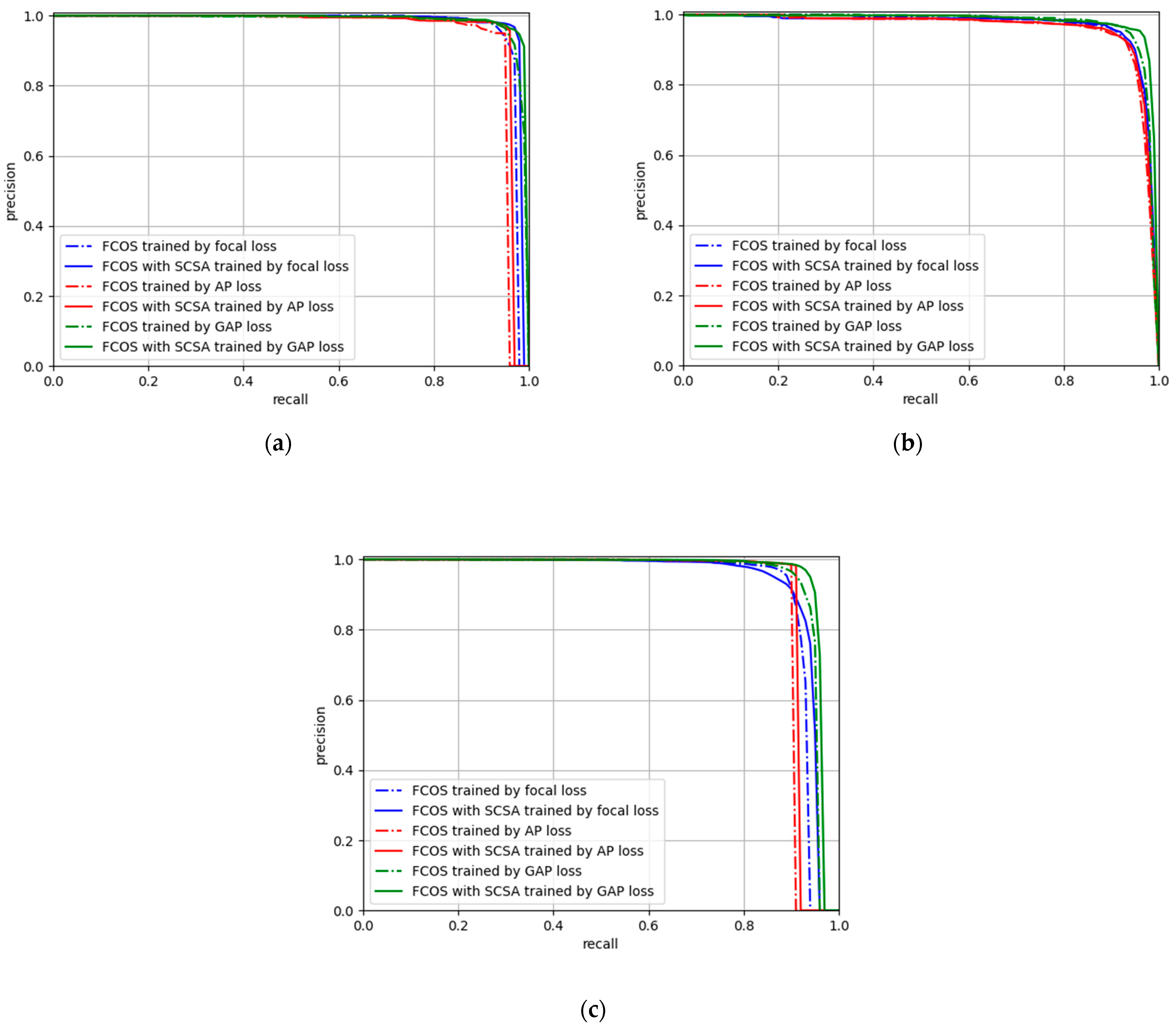
In this work, a one-stage anchor-free SCSA-Net is developed to accurately detect ship targets in SAR images. To improve the feature extraction ability of the network and reduce the interference of nearshore background to the ship target, an SCSA module is proposed to dynamically enhance the features in space. In addition, a GAP loss is proposed, which enables the network to optimize directly with AP as the target, and solves the “score shift” problem in AP loss, so that it can effectively improve the score of the predicted tar and promote the detection accuracy of the network. We can conclude the experimental results on SSDD, SAR-Ship-Dataset, and HRSID: (1) by using the SCSA module, the accuracy can be improved on all three datasets regardless of whether the training is performed using focal loss, AP loss, or GAP loss. Its effectiveness is confirmed; (2) by using GAP loss for training, the gap between the average classification scores of positive and negative samples can be effectively widened, and the accuracy can be improved with or without the SCSA module; (3) compared with other methods, the SCSA-Net proposed in this paper has higher detection accuracy on all three datasets.
Future work: our future work will focus on reducing the computing scale of the network without affecting its accuracy, and studying the application of arbitrarily oriented objects.

Author Contributions

Conceptualization, L.Z.; methodology, L.Z.; software, L.Z.; validation, L.Z. and Y.L.; formal analysis, L.Z. and Y.L.; investigation, L.Z.; resources, L.Z. and Y.L.; data curation, L.Z.; writing-original draft preparation, Y.L.; writing-review and editing, L.Z., Y.L., L.Q., J.C. and J.F.; visualization, L.Z. All authors have read and agreed to the published version of the manuscript.

Funding

This work was supported in part by the Xingliao Talents Program of Liaoning Province under Grant XLYC1907134, in part by the Scientific Research Project of the Department of Education of Liaoning Province under Grant LJKZ0174, and in part by Liaoning BaiQianWan Talents Program under Grant 2018B21.

Data Availability Statement

Not applicable.

Acknowledgments

We gratefully appreciate the publishers of the SSDD dataset, SAR-Ship-Dataset, and HRSID, and the editors and reviewers for their efforts and contributions.

Conflicts of Interest

The authors declare no conflict of interest.

References

  1. Zhang, P.; Xu, H.; Tian, T.; Gao, P.; Li, L.; Zhao, T.; Zhang, N.; Tian, J. SEFEPNet: Scale Expansion and Feature Enhancement Pyramid Network for SAR Aircraft Detection with Small Sample Dataset. IEEE J. Sel. Top. Appl. Earth Obs. Remote Sens. 2022, 15, 3365–3375. [Google Scholar] [CrossRef]
  2. Hong, Z.; Yang, T.; Tong, X.; Zhang, Y.; Jiang, S.; Zhou, R.; Han, Y.; Wang, J.; Yang, S.; Liu, S. Multi-Scale Ship Detection from SAR and Optical Imagery Via A More Accurate YOLOv3. IEEE J. Sel. Top. Appl. Earth Obs. Remote Sens. 2021, 14, 6083–6101. [Google Scholar] [CrossRef]
  3. Du, L.; Dai, H.; Wang, Y.; Xie, X.; Wang, Z. Target discrimination based on weakly supervised learning for high-resolution SAR images in complex scenes. IEEE Trans. Geosci. Remote Sens. 2020, 58, 461–472. [Google Scholar] [CrossRef]
  4. Li, X.; Li, D.; Liu, H.; Wan, J.; Chen, Z.; Liu, Q. A-BFPN: An Attention-Guided Balanced Feature Pyramid Network for SAR Ship Detection. Remote Sens. 2022, 14, 3829. [Google Scholar] [CrossRef]
  5. Li, S.; Fu, X.; Dong, J. Improved Ship Detection Algorithm Based on YOLOX for SAR Outline Enhancement Image. Remote Sens. 2022, 14, 4070. [Google Scholar] [CrossRef]
  6. Leng, X.; Ji, K.; Yang, K.; Zou, H. A Bilateral CFAR Algorithm for Ship Detection in SAR Images. IEEE Geosci. Remote Sens. Lett. 2015, 15, 1536–1540. [Google Scholar] [CrossRef]
  7. Ai, J.; Yang, X.; Song, J.; Dong, Z.; Jia, L.; Zhou, F. An Adaptively Truncated Clutter-Statistics-Based Two-Parameter CFAR Detector in SAR Imagery. IEEE J. Ocean. Eng. 2018, 43, 267–279. [Google Scholar] [CrossRef]
  8. Dai, H.; Du, L.; Wang, Y.; Wang, Z. A Modified CFAR Algorithm Based on Object Proposals for Ship Target Detection in SAR Images. IEEE Geosci. Remote Sens. Lett. 2016, 13, 1925–1929. [Google Scholar] [CrossRef]
  9. Li, N.; Pan, X.; Yang, L.; Huang, Z.; Wu, Z.; Zheng, G. Adaptive CFAR Method for SAR Ship Detection Using Intensity and Texture Feature Fusion Attention Contrast Mechanism. Sensors 2022, 22, 8116. [Google Scholar] [CrossRef]
  10. Li, M.; Cui, X.; Chen, S. Adaptive Superpixel-Level CFAR Detector for SAR Inshore Dense Ship Detection. IEEE Geosci. Remote Sens. Lett. 2022, 19, 4010405. [Google Scholar] [CrossRef]
  11. Girshick, R.; Donahue, J.; Darrell, T.; Malik, J. Rich Feature Hierarchies for Accurate Object Detection and Semantic Segmentation. In Proceedings of the 2014 IEEE Conference on Computer Vision and Pattern Recognition, Columbus, OH, USA, 23–28 June 2014; pp. 580–587. [Google Scholar] [CrossRef] [Green Version]
  12. Girshick, R. Fast R-CNN. In Proceedings of the 2015 IEEE International Conference on Computer Vision (ICCV), Santiago, Chile, 7–13 December 2015; pp. 1440–1448. [Google Scholar] [CrossRef]
  13. Ren, S.; He, K.; Girshick, R.; Sun, J. Faster R-CNN: Towards Real-Time Object Detection with Region Proposal Networks. IEEE Trans. Pattern Anal. Mach. Intell. 2017, 39, 1137–1149. [Google Scholar] [CrossRef] [PubMed] [Green Version]
  14. Sun, P.; Zhang, R.; Jiang, Y.; Kong, T.; Xu, C.; Zhan, W.; Tomizuka, M.; Li, L.; Yuan, Z.; Wang, C.; et al. Sparse R-CNN: End-to-End Object Detection with Learnable Proposals. In Proceedings of the IEEE/CVF Conference on Computer Vision and Pattern Recognition (CVPR), Nashville, TN, USA, 20–25 June 2021; pp. 14454–14463. [Google Scholar]
  15. Redmon, J.; Divvala, S.; Girshick, R.; Farhadi, A. You Only Look Once: Unified, Real-Time Object Detection. In Proceedings of the 2016 IEEE Conference on Computer Vision and Pattern Recognition (CVPR), Las Vegas, NV, USA, 27–30 June 2016; pp. 779–788. [Google Scholar] [CrossRef] [Green Version]
  16. Redmon, J.; Farhadi, A. YOLO9000: Better, Faster, Stronger. In Proceedings of the 2017 IEEE Conference on Computer Vision and Pattern Recognition (CVPR), Honolulu, HI, USA, 21–26 July 2017; pp. 6517–6525. [Google Scholar] [CrossRef] [Green Version]
  17. Redmon, J.; Farhadi, A. YOLOv3: An Incremental Improvement. arXiv 2018, arXiv:1804.02767. [Google Scholar] [CrossRef]
  18. Bochkovskiy, A.; Wang, C.; Liao, H. YOLOv4: Optimal Speed and Accuracy of Object Detection. arXiv 2020, arXiv:2004.10934. [Google Scholar] [CrossRef]
  19. Tang, G.; Liu, S.; Fujino, I.; Claramunt, C.; Wang, Y.; Men, S. H-YOLO: A Single-Shot Ship Detection Approach Based on Region of Interest Preselected Network. Remote Sens. 2020, 12, 4192. [Google Scholar] [CrossRef]
  20. Tang, G.; Zhuge, Y.; Claramunt, C.; Men, S. N-YOLO: A SAR Ship Detection Using Noise-Classifying and Complete-Target Extraction. Remote Sens. 2021, 13, 871. [Google Scholar] [CrossRef]
  21. Xie, F.; Lin, B.; Liu, Y. Research on the Coordinate Attention Mechanism Fuse in a YOLOv5 Deep Learning Detector for the SAR Ship Detection Task. Sensors 2022, 22, 3370. [Google Scholar] [CrossRef]
  22. Zhu, H.; Xie, Y.; Huang, H.; Jing, C.; Rong, Y.; Wang, C. DB-YOLO: A Duplicate Bilateral YOLO Network for Multi-Scale Ship Detection in SAR Images. Sensors 2021, 21, 8146. [Google Scholar] [CrossRef]
  23. Liu, W.; Anguelov, D.; Erhan, D.; Szegedy, C.; Reed, S.E.; Fu, C.Y.; Berg, A.C. SSD: Single Shot MultiBox Detector. In Proceedings of the European Conference on Computer Vision, Amsterdam, The Netherlands, 8–16 October 2016; pp. 21–37. [Google Scholar] [CrossRef] [Green Version]
  24. Lin, T.Y.; Goyal, P.; Girshick, R.; He, K.; Dollár, P. Focal loss for dense object detection. In Proceedings of the IEEE International Conference on Computer Vision, Venice, Italy, 22–29 October 2017; pp. 2980–2988. [Google Scholar] [CrossRef] [Green Version]
  25. Tian, Z.; Shen, C.; Chen, H.; He, T. FCOS: Fully Convolutional One-Stage Object Detection. In Proceedings of the 2019 IEEE/CVF International Conference on Computer Vision (ICCV), Seoul, Republic of Korea, 27–28 October 2019; pp. 9626–9635. [Google Scholar] [CrossRef] [Green Version]
  26. Li, J.; Qu, C.; Shao, J. Ship detection in SAR images based on an improved faster R-CNN. In Proceedings of the 2017 SAR in Big Data Era: Models, Methods and Applications (BIGSARDATA), Beijing, China, 13–14 November 2017; pp. 1–6. [Google Scholar] [CrossRef]
  27. Wang, Y.; Wang, C.; Zhang, H.; Dong, Y.; Wei, S. A SAR Dataset of Ship Detection for Deep Learning under Complex Backgrounds. Remote Sens. 2019, 11, 765. [Google Scholar] [CrossRef] [Green Version]
  28. Wei, S.; Zeng, X.; Qu, Q.; Wang, M.; Su, H.; Shi, J. HRSID: A High-Resolution SAR Images Dataset for Ship Detection and Instance Segmentation. IEEE Access. 2020, 8, 120234–120254. [Google Scholar] [CrossRef]
  29. Zhang, T.; Zhang, X.; Li, J.; Xu, X.; Wang, B.; Zhan, X.; Xu, Y.; Ke, X.; Zeng, T.; Su, H.; et al. SAR Ship Detection Dataset (SSDD): Official Release and Comprehensive Data Analysis. Remote Sens. 2021, 13, 3690. [Google Scholar] [CrossRef]
  30. Shi, H.; Fang, Z.; Wang, Y.; Chen, L. An Adaptive Sample Assignment Strategy Based on Feature Enhancement for Ship Detection in SAR Images. Remote Sens. 2022, 14, 2238. [Google Scholar] [CrossRef]
  31. Cui, Z.; Li, Q.; Cao, Z.; Liu, N. Dense Attention Pyramid Networks for Multi-Scale Ship Detection in SAR Images. IEEE Trans. Geosci. Remote Sens. 2019, 57, 8983–8997. [Google Scholar] [CrossRef]
  32. Zhang, T.; Zhang, X.; Ke, X. Quad-FPN: A Novel Quad Feature Pyramid Network for SAR Ship Detection. Remote Sens. 2021, 13, 2771. [Google Scholar] [CrossRef]
  33. Zhu, M.; Hu, G.; Li, S.; Zhou, H.; Wang, S.; Feng, Z. A Novel Anchor-Free Method Based on FCOS + ATSS for Ship Detection in SAR Images. Remote Sens. 2022, 14, 2034. [Google Scholar] [CrossRef]
  34. Wu, Z.; Hou, B.; Ren, B.; Ren, Z.; Wang, S.; Jiao, L. A Deep Detection Network Based on Interaction of Instance Segmentation and Object Detection for SAR Images. Remote Sens. 2021, 13, 2582. [Google Scholar] [CrossRef]
  35. Wang, R.; Shao, S.; An, M.; Li, J.; Wang, S.; Xu, X. Soft Thresholding Attention Network for Adaptive Feature Denoising in SAR Ship Detection. IEEE Access 2021, 9, 29090–29105. [Google Scholar] [CrossRef]
  36. Tian, L.; Cao, Y.; He, B.; Zhang, Y.; He, C.; Li, D. Image Enhancement Driven by Object Characteristics and Dense Feature Reuse Network for Ship Target Detection in Remote Sensing Imagery. Remote Sens. 2021, 13, 1327. [Google Scholar] [CrossRef]
  37. Wei, S.; Su, H.; Ming, J.; Wang, C.; Yan, M.; Kumar, D.; Shi, J.; Zhang, X. Precise and Robust Ship Detection for High-Resolution SAR Imagery Based on HR-SDNet. Remote Sens. 2020, 12, 167. [Google Scholar] [CrossRef] [Green Version]
  38. Ashish, V.; Noam, S.; Niki, P.; Jakob, U.; Llion, J.; Aidan, N.G.; Lukasz, K.; Illia, P. Attention Is All You Need. In Proceedings of the Advances in Neural Information Processing Systems, Long Beach, CA, USA, 4–9 December 2017. [Google Scholar]
  39. Chen, K.; Li, J.; Lin, W.; See, J.; Wang, J.; Duan, L.; Chen, Z.; He, C.; Zou, J. Towards Accurate One-Stage Object Detection With AP-Loss. In Proceedings of the IEEE/CVF Conference on Computer Vision and Pattern Recognition (CVPR), Long Beach, CA, USA, 15–20 June 2019; pp. 5119–5127. [Google Scholar]
  40. Lin, Z.; Ji, K.; Leng, X.; Kuang, G. Squeeze and Excitation Rank Faster R-CNN for Ship Detection in SAR Images. IEEE Geosci. Remote Sens. Lett. 2019, 16, 751–755. [Google Scholar] [CrossRef]
Figure 1. Overview of our proposed SCSA-Net. It consists of four sections: the backbone of the SCSA-Net, feature pyramid network (FPN), spatial cross-scale attention module, and class-box subnet.
Remotesensing 15 00350 g001
Figure 2. The structure of the cross-scale attention module.
Remotesensing 15 00350 g002
Figure 3. The structure of the spatial attention redistribution module.
Remotesensing 15 00350 g003
Figure 4. Curves of the average classification scores of positive and negative samples output from the network trained by focal loss during the training phase.
Remotesensing 15 00350 g004
Figure 5. Curves of the average classification scores of positive and negative samples output from the network trained by AP loss during the training phase.
Remotesensing 15 00350 g005
Figure 6. Curves of the average classification scores of positive and negative samples output from the network trained by GAP loss during the training phase.
Remotesensing 15 00350 g006
Figure 7. Precision-Recall curves (PR curves) of SCSA-Net with different settings. (a) PR curves of SCSA-Net with different settings on SSDD. (b) PR curves of SCSA-Net with different settings on SAR-Ship-Dataset. (c) PR curves of SCSA-Net with different settings on HRSID.
Remotesensing 15 00350 g007
Figure 8. Visualization results of ablation experiments on the SSDD. (a) Ground truths. (b) Detection results of FCOS trained by focal loss. (c) Detection results of FCOS trained by GAP loss. (d) Detection results of FCOS with SCSA module trained by GAP loss.
Remotesensing 15 00350 g008aRemotesensing 15 00350 g008b
Figure 9. Visualization results of ablation experiments on the SAR-Ship-Dataset. (a) Ground truths. (b) Detection results of FCOS trained by focal loss. (c) Detection results of FCOS trained by GAP loss. (d) Detection results of FCOS with SCSA module trained by GAP loss.
Remotesensing 15 00350 g009aRemotesensing 15 00350 g009bRemotesensing 15 00350 g009c
Figure 10. Visualization results of ablation experiments on the HRSID. (a) Ground truths. (b) Detection results of FCOS trained by focal loss. (c) Detection results of FCOS trained by GAP loss. (d) Detection results of FCOS with SCSA module trained by GAP loss.
Remotesensing 15 00350 g010aRemotesensing 15 00350 g010b
Figure 11. Comparison of the results of different methods. (a) Ground truths. (b) Detection results of HR-SDNet. (c) Detection results of ResNet-50+Quad-FPN. (d) Detection results of SCSA-Net.
Remotesensing 15 00350 g011aRemotesensing 15 00350 g011b
Figure 12. PR curves of different methods. (a) PR curves of different methods on SSDD. (b) PR curves of different methods on SAR-Ship-Dataset. (c) PR curves of different methods on HRSID.
Remotesensing 15 00350 g012aRemotesensing 15 00350 g012b
Table 1. Ablation study of SCSA-Net on SSDD, SAR-Ship-Dataset, and HRSID.
BaselineDifferent Settings of SCSA-Net
Focal loss
AP loss
GAP loss
SCSA
SSDD96.594.598.097.295.598.7
SAR-Ship-Dataset96.195.497.096.395.897.9
HRSID92.089.994.293.290.995.4
√ indicates that the corresponding item is used. The best results are bolded.
Table 2. Results of different settings of SCSA module on SSDD, SAR-Ship-Dataset, and HRSID.
Different Settings of SCSA Module
A s 1
A s 2
SSDD98.47598.57198.59198.745
SAR-Ship-Dataset97.57197.75897.76697.882
HRSID95.04695.20395.23095.392
√ indicates that the corresponding item is used. The best results are bold.
Table 3. Comparison with the latest SAR ship detection methods on SSDD.
MethodsAP
Two-stageFaster R-CNN [13]90.8
SER Faster R-CNN [40]91.5
ISASDNet+r50 [34]95.4
ISASDNet+r101 [34]96.8
STANet-50+FPN [35]95.7
Mask-RCNN(OCIE-DFR-RFE) [36]92.1
One-stageResNet-50+Quad-FPN [32]96.6
YOLOV3 (OCIE-DFR-RFE) [36]68.8
ASAFE [30]95.2
A-BFPN [4]96.8
HR-SDNet [37]89.4
Unnamed method * [33]98.4
ours98.7
* indicates that the authors of this paper did not name the proposed overall method. The best result is bold.
Table 4. Comparison with the latest SAR ship detection methods on SAR-Ship-Dataset.
MethodsAP
Two-stageFaster R-CNN [13]91.7
SER Faster R-CNN [40]92.2
ISASDNet+r50 [34]95.3
ISASDNet+r101 [34]95.8
One-stageResNet-50+Quad-FPN [32]94.4
HR-SDNet [37]92.3
ours97.9
The best result is bold.
Table 5. Comparison with the latest SAR ship detection methods on HRSID.
MethodsAP
Two-stageFaster R-CNN [13]80.7
SER Faster R-CNN [40]81.5
One-stageResNet-50+Quad-FPN [32]90.9
HR-SDNet [37]85.9
ours95.4
The best result is bold.
Table 6. The number of parameters of each module and the testing speed of the network.
Backbone (ResNet-50)FPNSCSA ModuleClass-Box SubnetTotal Param(M)FPS
Param(M)23.453.879.614.74--
FCOS 32.0630
SCSA-Net41.6722
√ indicates that the corresponding item is used.
Disclaimer/Publisher’s Note: The statements, opinions and data contained in all publications are solely those of the individual author(s) and contributor(s) and not of MDPI and/or the editor(s). MDPI and/or the editor(s) disclaim responsibility for any injury to people or property resulting from any ideas, methods, instructions or products referred to in the content.

