Monitoring Urban Expansion by Coupling Multi-Temporal Active Remote Sensing and Landscape Analysis: Changes in the Metropolitan Area of Cordoba (Argentina) from 2010 to 2021

Abstract

Uncontrolled and unsustainable urban sprawl are altering the Earth’s surface at unprecedented rates. This research explores the potential of active remote sensors for mapping urban areas, for monitoring urban expansion processes and for depicting landscape pattern dynamics in a metropolis of South America. Based on multi-temporal urban cover maps of Cordoba, Argentina, purposely derived from COSMO-SkyMed SAR data by urban extraction algorithms, we quantified urban surface increase and described urbanization processes that occurred during 2010–2021 in sectors with different degrees of soil sealing. We extracted urban extent in four time-steps using an Urban EXTent extraction (UEXT) algorithm and quantified urban expansion, identifying newly built areas on 2.5 ha cells. For these cells, we computed urban cover and a set of landscape pattern indices (PIs), and by projecting them in a composition vs. configuration Cartesian space we performed a trajectory analysis. SAR-based urban extraction and cover change proved to be very accurate. Overall accuracy and Cohen’s Kappa statistic evidenced very high values, always above 91.58% and 0.82, respectively, for urban extraction, and also above 90.50% and 0.72 concerning the accuracy of urban expansion. Cordoba’s urban surface significantly increased (≈900 ha in 10 years) following three main spatial processes in different city sectors (e.g., edge-expansion and outlying on peri-urban areas, and infill inside the ring road), which may have contrasting effects on the sustainability of the metropolitan area. Trajectory analysis highlighted non-linear relations between the urban cover and the PIs. Areas with very low and low urban intensity underwent a steep rise of both urban cover and PI values (e.g., urban patch dimension, complexity and number), depicting urban edge-expansion and outlying processes. In the areas with medium and high urban intensity the increase in patch dimension, along with the decrease in patch number and complexity, evidence the coalescence of urban areas that incorporate in the urban fabric the remnants of non-built up zones and fill the few residual green spaces. The proposed SAR mapping procedure coupled with landscape analysis proved to be useful to detect and depict different moments of urban expansion and, pending more tests on other cities and geographical conditions, it could be postulated among the RS indicators to monitor the achievement of the Sustainable Development Goals established by the United Nations.

1. Introduction

The continuous and persistent population growth that, in the last century, has further raised worldwide, has promoted a consistent expansion of built-up areas at the expense of natural, semi-natural and agricultural environments [1]. During the last seventy years, an intense migratory movement from rural to urban areas has occurred and since, in 2008, half of the world’s population lived in cities, recent projections suggest that by 2050 human populations living in urban areas will reach the level of 68% [2]. Urban expansion is one of the major drivers of global change, causing important direct and indirect impacts on environmental conditions and biodiversity at multiple scales [3]. Land take often causes irreversible environmental changes due to the replacement of natural and semi-natural ecosystems by impervious surfaces [4]. Urbanization modifies environmental conditions, directly altering several ecosystem processes such as hydrological balance [5], biogeochemical cycles [6], land surface temperature and local meteorological conditions [7], and several related ecosystem services [8]. Urban expansion is one of the primary drivers of habitat loss and species extinction [9], and it has several indirect environmental impacts such as the intensification of global greenhouse gas emissions, the increase in pollution levels and the alteration of residual natural ecosystems [10].

Identifying adequate management and governance strategies for a correct development of urban areas is a crucial challenge of the Anthropocene Epoch. In consideration of these challenges, the United Nations have included innovative management and governance strategies in the Sustainable Development Agenda for 2030 (so called SDG 2030) [11]. The 11th SDG goal states: “make cities and human settlements inclusive, safe, resilient and sustainable” and intends to promote sustainable urban planning and management by improving environmental infrastructures (e.g., water, urban green, drainage and solid waste management), developing a sustainable construction industry and promoting sustainable systems of energy and transport. The achievement of the 11th SDG goal requires important efforts for identifying effective monitoring tools able to depict urban changes and to support policy makers [12].

In this context, good support could be given by Remote Sensing (RS), which offers multi-temporal data at different spatial scales in a cost-effective, spatially contiguous and timely manner, allowing the standardized detection of urban areas and urbanization processes [13,14]. RS data are a promising support for quantifying urban growth in all its various forms (e.g., infill, edge-expansion, and outlying) [15].

RS applications for urban change analysis were traditionally based on time series of medium resolution data registered with multi-spectral optical sensors as Landsat [16,17,18,19], SPOT [20,21], Sentinel-2 [22], or the combination of two or more sensors [12,23]. Nevertheless, multi-spectral RS data could present some limitations due to technical constraints such as atmospheric and light conditions (e.g., cloud percentage and night hours), in which passive sensors are unable to acquire data [13]. Furthermore, mapping transitions among urban and semi-natural landscapes using satellite passive data had some constraints on discriminating built-up areas from bare rock or wasteland, mainly because of the insufficient spatial and/or spectral resolution [24]. Another possible approach for quantifying urban expansion could be based on nighttime lights sensors (e.g., DSMP-OLS satellite) [25,26], but this presents similar shortcomings due to atmospheric conditions (e.g., clouds) and coarse spatial resolutions [27,28]. On the other hand, remote sensed data registered by Synthetic Aperture Radar (SAR) sensors as Envisat [29], Sentinel-1 [30], or TerraSAR-X [31] seem very promising as SAR data overcome some atmospheric constrains (such as clouds or light), offer very high spatial resolution (VHR; e.g., less than 5 meters) and are supported by several satellite platforms (e.g., TerraSAR-X, Cosmo-SkyMed, Radarsat-2, etc.).

The use of VHR SAR data for producing accurate urban maps has been explored and tested and its effectiveness for urban extraction and mapping relies on signal features (e.g., the double bounce backscatter effect and the temporal stability that characterizes SAR data in correspondence with urban areas and buildings) [32]. SAR features allow built-up areas to be clearly distinguished from other cover types [33] and VHR allows urban edges to be accurately outlined [34]. However, to date, the use of multi-temporal VHR SAR data to analyze urban expansion is still limited, and their application in South American cities is rare [29,35].

South America, and in particular Argentina, has registered a consistent rise in population and an uncontrolled urban expansion during the last century [36]. Over 92% of the Argentinean population lives in urban areas which makes this country one of the most urbanized regions in the world [37]. In this context, the peri-urban zones composed by natural, semi-natural, and agricultural areas have been affected by a rapid and uncontrolled land use change process, with new built-up areas and land take [38,39]. Although several studies have analyzed the effects of this uncontrolled urbanization on different natural and seminatural ecosystems [38,40], animal communities [41] or socio-economic impacts [42], a landscape approach to examine the urbanization rates on city sectors with different degrees of urban intensity has not been carried out yet. The analysis of urban land patterns over time is crucial to better understand the incidence of built-up areas on the overall city and may supply monitoring indicators for the assessment of Sustainable Developments Goals. In this context, landscape trajectory analysis, depicting urban spatial patterns over time, could be an efficient approach for analyzing urbanization processes occurring in cities and metropolitan areas [43]. The trajectory analysis aids in the depiction of the different ways in which urban expansion occurs (e.g., infill, edge-expansion, and outlying) inside the city and in peri-urban areas, offering insights on the sustainability of the urbanization process [15,43]. Trajectory analysis was developed to monitor landscape change over time, based on continuous or multi-temporal remote sensing data [44]. This method was applied to several variables as backscatter values derived by SAR satellites [45], surface temperature [46], spectral indices [47] or landscape metrics [48,49], and to very different environments (e.g., forest, urban, and agricultural). To date, most applications of trajectory analysis on urban contexts are supported by multi-spectral optical sensors with medium resolution (e.g., Landsat data), whereas the use of SAR data is still limited [44,50,51].

In consideration of the above, the present work aims at examining urbanization processes detected by SAR multi-temporal satellite images occurring in a subtropical big city of South America during the last decade (2010–2021). The research, based on purposefully produced multi-temporal urban maps (2010, 2012–2013, 2018–2019, 2020–2021) of the metropolitan landscape of Cordoba (the second city by number of inhabitants of Argentina), aims at: (i) depicting urban cover over time and detecting the new built-up zones; (ii) quantifying the intensity and extension of land take; (iii) describing, through trajectory analyses, urban cover and spatial configuration over the last decade in the overall city and in sectors characterized by different soil sealing degree (%) defined as urban intensity (very low, low, medium, high), (iv) identifying different urban expansion processes [15] across the city as mapping infill, edge-expansion, and outlying areas may support sustainable planning. This research, based on standard SAR images elaboration, also contributes to better explore the usefulness of active remote sensed data for mapping and monitoring urban areas and their dynamic processes, offering further tools and indicators to assess the achievement of Goal 11 for Sustainable Development established by the United Nations [12].

2. Materials and Methods

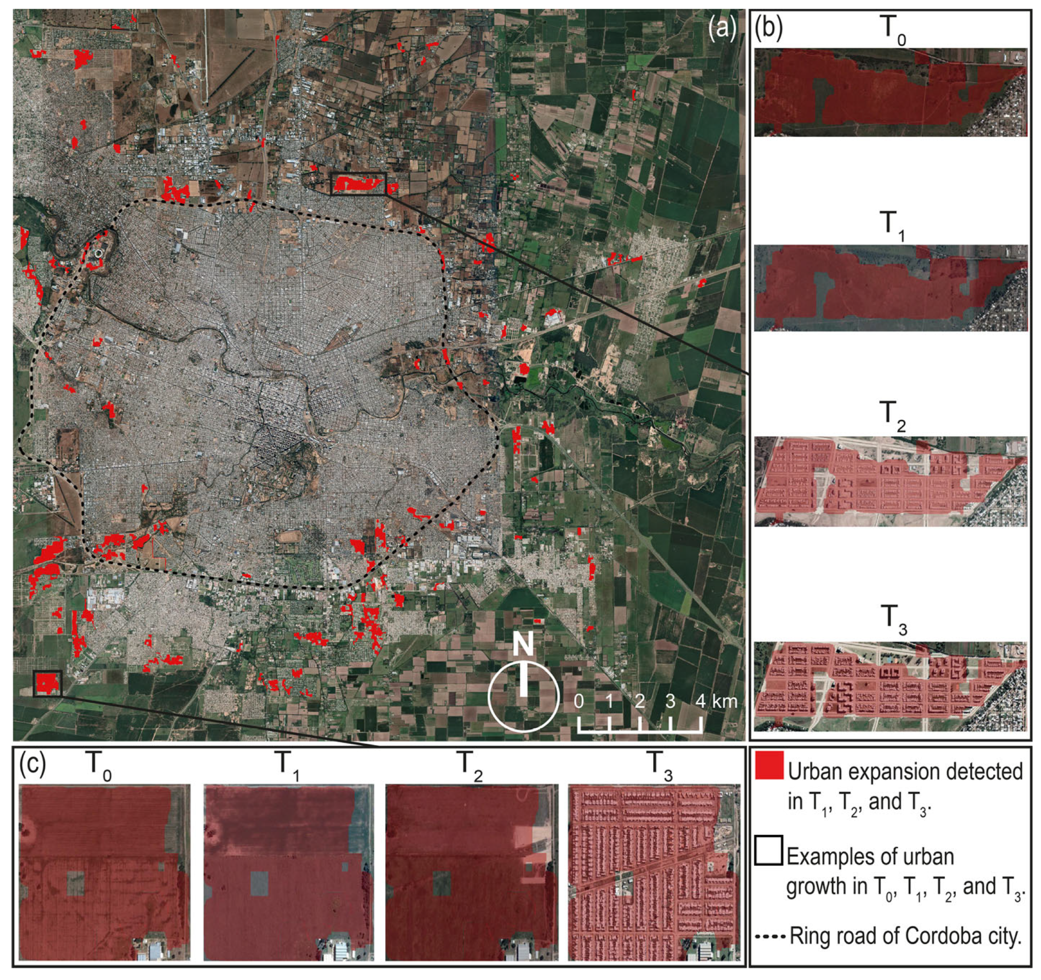
2.1. Study Area

The study was implemented in the metropolitan area of Cordoba (Central Argentina, Figure 1), which is the capital of the homonymous province and, with more than 1.3 million inhabitants in 2014 and an average annual increase of 1%, is the second most populous city in Argentina [52]. Cordoba city is placed in an area of plains, with elevations ranging from 360 to 480 m above sea level. Its climate is temperate and semi-dry, with mean annual precipitations of ≈800 mm concentrated in summer. The monthly average temperature ranges from 14.8 °C in winter to 22.7 °C in summer [53]. Cordoba is undergoing a consistent process of urban growth on its periphery that occurs at the expense of agricultural fields and forestry patches [52]. Its current extension is over 35 ha, with a density of 57 persons per ha [4,52]. The population of the Cordoba province has increased during the last seventy years, and it is expected to grow further in the future (https://estadistica.cba.gov.ar/conoce-cordoba/ (accessed on 10 October 2022)).

2.2. Data Collection and Analysis

We detected and analyzed the urbanization process of the metropolitan area of Cordoba during the last decade, following a sequence of steps schematically reported in Figure 2: (A) SAR satellite image selection and pre-processing, (B) urban area extraction and accuracy assessment, (C) urban expansion detection and accuracy analysis, (D) urban trajectory analysis.

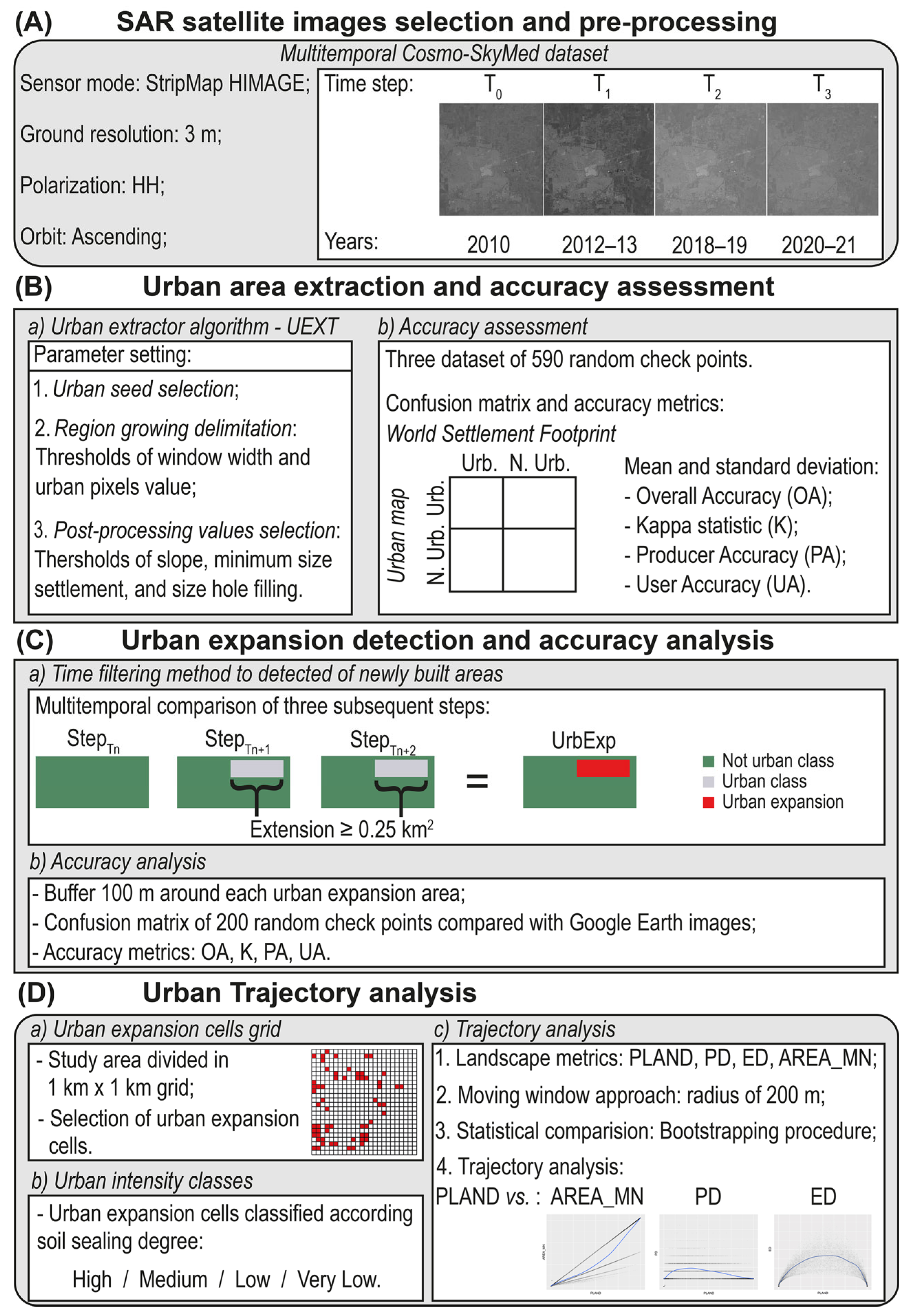
2.2.1. SAR Satellite Images Selection and Pre-Processing

For SAR satellite image selection and pre-processing (Figure 2, box A), we downloaded 12 CSK images from the Cosmo-SkyMed portal (https://portal.cosmo-skymed.it (accessed on 12 September 2022)), acquired in the period 2010–2021, in Stripmap Himage mode with 3 m spatial resolution in ascending orbit and HH polarization. The Cosmo-SkyMed (CSK) constellation (Italian Space Agency—ASI) includes four first generation satellites (first launched 8 June 2007) and five second generation satellites (first launched 18 December 2019) equipped with a multi-mode and multi-polarization (HH, HV, VV, VH) very high-resolution SAR operating at X-band [54,55].

The selected images were radiometrically calibrated and geocoded using the Shuttle Radar Topography Mission (SRTM) with 90 m by ASI (Table S1, Figure 2 box A) [56]. The terrain backscattering coefficients (σ₀) were extracted, exploiting the procedure, and numbers reported in the official mission document [56]. To reduce the speckle noise, each CSK image was filtered according the RABASAR algorithm [57], a ratio-based multitemporal denoising framework based on the use of a ratio image composed of a noisy image and the temporal mean of the stack.

The CSK images were grouped in four time intervals (T₀: 2010, T₁: 2011–2012, T₂: 2018–2019, and T₃: 2020–2021) and for each interval the mean backscatter values are computed and considered, as opposed to keeping the images separated (Figure 2 box A). We adopted multitemporal maps as a sound support for trajectory analysis [44].

2.2.2. Urban Area Extraction and Accuracy Assessment

We extracted urban area extents (Figure 2 box B) for each time period using the Urban EXTent extraction (UEXT) algorithm [58]. The UEXT algorithm assumes that built-up structures are subject to double bounce effects and their pixels are characterized by high intense backscatter values that are stable over time [32]. The UEXT algorithm reduces the false positives pixels (e.g., rocks), masking pixels with very high slopes (20 degrees in this work) where built-up structures are not feasible [59]. This “slope threshold” is designed using the Digital Elevation Model of SRTM at 30 m spatial resolution [59]. This urban extraction approach was implemented in Google Earth Engine (GEE). The implementation of the UEXT algorithm is structured in three phases (Figure 2 box B.a) [58,60]:

• Urban seed selection: selection of a set of very likely urban pixels with very high backscatter values above a “seed threshold”.
• Region growing: delimitation of a growing region window of 3 km around each “seed threshold” and the addition inside it of further urban pixels to the original seed points. The addition of urban pixels was performed by a flooding algorithm computed by summing up pixels iteratively with high intensity values (≥“seed threshold”). This algorithm assumes that different man-made elements in an image are characterized by similar levels of backscattering. This iterative procedure is repeated as long as the cumulative sum of the urban pixels’ backscattered values results below the “urban threshold” value, which in this work is set to 1000 for Cosmo images of the first generation and to 800 for Cosmo images of the second generation.
• Post-processing: pixels located on too high slope values (above the “slope threshold” of 20 degrees) are discarded, as well as “salt and pepper” classification errors. The latter is carried out by means of a hole filling procedure using two morphological parameters: “minimum size settlements” and “size hole filling”. Both procedures aim at improving the mapping of built-up areas and the discrimination of built-up structures from parks, ponds, or bare soil.

The urban extent maps were extracted using different combinations of UEXT algorithm values. The “seed threshold” was defined between −3 and 3, the range of “urban threshold” varied from 600 to 2000, and the “minimum size settlement” and “size hole filling” ranges from 10 to 100. We adopted different combinations of these parameters by tuning them at different steps intervals (see Table S2), and based on the higher accuracy values (Overall Accuracy and Cohen’s Kappa statistic) we chose the best combination as follows: “Seed threshold” was set to −2 for Cosmo images of first generation (T₀, T₁, T₂) and to 1 for Cosmo images of second generation (T₃); for “urban threshold” the best values were established as 1000 for Cosmo images of the first generation and to 800 for Cosmo images of the second generation; and “minimum size settlements” and “size hole filling” were fixed to 20 in Cosmo images of the first generation and of 15 in Cosmo images of the second generation.

The accuracy of the urban extent maps (Figure 2, box B.b) was assessed through the computation of the following indexes: Overall Accuracy (OA), Cohen’s Kappa statistic (K), Producer Accuracy (PA), and User Accuracy (UA) [61]. The Overall Accuracy (OA) is a measure of the overall effectiveness of extraction, and its values range from 0%, total absence of accuracy, to 100%, a perfect urban extraction. OA values greater than 85% are considered as acceptable results. The Producer Accuracy (PA) refers to the probability of a built-up structure being correctly extracted, and the User Accuracy to the probability of a pixel extracted as urban of being truly a built-up structure. PA and UA values range from 0%, with incorrect extraction, to 100%: built-up structures perfectly extracted. An urban extraction presenting PA and UA values over 80% shows a very low probability of error [61]. The Cohen’s Kappa metric (K) measures the agreement between urban extraction and the checkpoints and express degree of reliability of the urban map [61]. K values range from 0 (no reliability) to 1 (perfect reliability), and Landis and Koch [62] suggest the following ranges: K ≥ 0.80: almost perfect reliability, 0.60 ≤ K < 0.80: substantial reliability, 0.40 ≤ K < 0.60: moderate reliability, 0.20 ≤ K < 0.40: fair reliability, and K ≤ 0.20: slight or poor reliability.

The obtained urban extents were compared with the World Settlement Footprint (WSF) 2015 and 2019, which are accurate urban classifications produced at the global scale using multispectral and SAR sensors [63,64]. For a reliable accuracy assessment of built-up area maps, we used three independent sets of 590 randomly selected points for each time map, computing for each of them the above-mentioned accuracy metrics and eventually obtaining their mean and standard deviation values. Confusion matrices are based for T₀ and T₁ extractions on WSF-2015 and for T₂ and T₃ maps on WSF-2019. To correct possible errors of the WSF, caused by temporal shifts, the checkpoints for each time step were visually checked on coeval aerial orthophotos with very high spatial resolution (~30 cm), freely available on Google Earth (Table S3).

2.2.3. Urban Expansion Detection and Accuracy

To detect urban expansion (Figure 2 box C.a) in each time period (UrbExp_Tn), we used a time filtering method based on the comparison of a series of three successive urban maps [65]. We considered as a real urban expansion only in those areas classified as not urban in a given time step (NU_Tn), and as urban in the successive two ones (U_Tn+1 and U_Tn+2). For instance, UrbExp_T1 = NU_T0 followed by U_T1 and U_T2; UrbExp_T2 = NU_T1 followed by U_T2 and U_T3; and UrbExp_T3 = NU_T1 followed by NU_T2 and U_T3. To reduce false positives, a conservative approach was adopted, and expansion areas smaller than 2.5 ha were excluded [66].

The accuracy of the detected urban expansion maps (Figure 2 box C.b) was further validated through confusion matrices and by calculating the OA, K, PA, UA metrics on different validation data sets. Specifically, after setting a buffer of 100 m around each urban expansion area, including stable and changing areas, 200 randomly selected checkpoints inside this buffer were analyzed. For each point, a multi-temporal visual inspection using Google Earth aerial orthophotos for the analyzed period was performed in order to classify them in two categories: UrbExp_Tn and NUrbExp_Tn, or urban and not urban expansion at time interval T_n, respectively.

2.2.4. Urban Trajectory Analysis

Finally, urban area extents were analyzed by trajectory analysis along the time series (Figure 2 box D), an approach effectively used to depict the relationship between landscape composition (proportion of land-use types) and configuration (spatial arrangement of land-use types) [67] on natural and heterogeneous landscapes [40,68]. Trajectory analysis, here implemented on artificial contexts, could help to better understand the relationships between built-up areas’ composition and configuration, thus offering new insights to interpret and model urban changes and answering the great need of sustainability indicators for cities [69]. The trajectory analysis offers a sound workflow to investigate the non-linear relationship among landscape composition and configuration, and to better interpret urban configuration values across urban cover gradients. The trajectory analysis was performed in three steps, as follows (Figure 2 box D):

• Urban expansion cells grid: the metropolitan area of Cordoba was subdivided into a regular square grid of 100 ha (Figure 2 box D.a). The use of a regular grid allows spatio-temporal information on a set of zones with the same size to be obtained, supporting statistical comparisons [70]. A 100 ha grid size can be considered an appropriate scale to analyze urban dynamics in a large city such as Cordoba [70]. For statistical analysis, only cells in which urban expansion (UrbExp) had been detected were considered.
• Urban intensity classes: The 100 ha selected UrbExp grid cells were classified according to their urban intensity in terms of soil sealing degree (Figure 2 box D.b) [71]. The Copernicus Urban Atlas classification scheme was adopted, because it is a standard frame for land monitoring in Europe (Copernicus Land Monitoring Service available at: https://www.eea.europa.eu/data-and-maps/data/copernicus-land-monitoring-service-urban-atlas (accessed on 24 October 2022)). We identified the following four urban intensity classes (see also Table S4): Very Low (soil sealing degree ≤ 10%), Low (10% < soil sealing degree ≤ 30%), Medium (30% < soil sealing degree ≤ 50%), High (soil sealing degree > 50%).
• Trajectory analysis: A set of four non-redundant landscape metrics (Figure 2 box D.c;

  Table 1. Computed landscape parameters reporting the relative acronym, formula, description, unit of measure and landscape pattern facet. PLAND = urban area, NP = number of urban patches, PD = urban patches’ density, ED = urban edges’ density, AREA_MN = mean urban patch area.

  Acronym	Formula	Description	Unit	Landscape Pattern Facet
  PLAND	$\frac{{{\displaystyle \sum }}_{\mathrm{i}=1}^{\mathrm{n}}{\mathrm{a}}_{\mathrm{i}}}{\mathrm{A}}*100$	Proportion of landscape occupied by urban class. Measure of dominance.	Percent (%)	Composition
  PD	$\frac{\mathrm{n}}{\mathrm{A}}$	Number of urban patches per unit area. Measure of urban sprawl.	Number per hectare	Configuration
  ED	$\frac{{{\displaystyle \sum }}_{\mathrm{i}=1}^{\mathrm{n}}{\mathrm{e}}_{\mathrm{i}}}{\mathrm{A}}$	Total edge length of urban patches per unit area. Measure of urban areas’ shape complexity.	Meters per hectare	Configuration
  AREA_MN	$\frac{{{\displaystyle \sum }}_{\mathrm{i}=1}^{\mathrm{n}}{\mathrm{a}}_{\mathrm{i}}}{\mathrm{NP}}$	Average area of urban areas weighted by the number of urban patches. Measure of the degree of urbanization.	Hectares	Configuration

  a_i = area of the i-th urban patch, A = total landscape area, n = number of urban patches, e_i = total length of the i-th urban patch edge, NP= number of urban patches.

  ) were selected to estimate landscape composition and configuration at each time step [72,73]. We computed for each UrbExp grid cell the percentage of landscape covered by built-up structures (PLAND); the patch density (PD), describing the number of urban patches per unit area; the edge density (ED), which measures overall shape complexity defined as the total edge length of urban patches per unit area; and the mean patch area (AREA_MN), which depicts the average extension of urban patches per unit area (Table 1) [74].

Landscape metrics, computed by a moving window approach implemented for each time period, were obtained for each urban expansion cell and for soil sealing classes (Figure 2 box D.c) [75]. To better depict the pattern of the analyzed urban landscape, we set the radius of the moving window to 200 m, twice the regular street block characterizing the metropolitan area of Cordoba (100 m).

The differences in urban composition and configuration measured by PLAND, AREA_MN, PD, and ED were estimated using a nonparametric bootstrapping test of the mean cell values (Figure 2 box D.c) [33,76]. Bootstrapping significances with 95% confidence intervals were computed for both the overall urban expansion cells (UrbExp_Tn) and for each urban intensity class extracted at T₀ (Very Low, Low, Medium, High).

The temporal trajectories were assessed by describing the displacement into the specific relationship spaces (e.g., composition vs. configuration) of the mean metric values (e.g., PLAND vs. PD, PLAND vs. ED, PLAND vs. AREA_MN) [76] measured for the different time-steps [40,68,77].

3. Results

3.1. Urban Area Extraction and Accuracy Assessment

The UEXT algorithm allowed the mapping of the urban extents of Cordoba with very high accuracy in all the analyzed time periods (Figure 3 and

Table 2. Accuracy assessment of urban area extent maps obtained by applying UEXT to CSK data at T₀, T₁, T₂ and T₃.

Step	OA (%)	K	Urb. UA (%)	Urb. PA (%)	N. Urb. UA (%)	N. Urb. PA (%)
T0	94.75 ± 0.74	0.88 ± 0.02	92.39 ± 3.39	91.92 ± 1.65	95.75 ± 1.23	96.24 ± 0.59
T1	91.98 ± 1.95	0.83 ± 0.05	84.55 ± 5.86	94.90 ± 1.93	96.95 ± 0.53	90.26 ± 0.02
T2	91.58 ± 0.99	0.82 ± 0.03	87.84 ± 5.50	88.68 ± 1.56	93.41 ± 1.70	93.21 ± 1.25
T3	93.62 ± 0.20	0.86 ± 0.01	94.06 ± 3.28	88.17 ± 0.94	93.17 ± 1.68	96.90 ± 1.19

), with very high overall accuracy values (always OA ≥ 91.58%) and almost perfect reliability (always K ≥ 0.82, Table 2). The probability that a pixel classified as urban represents a real built-up structure is very high (UA values between 84.55% at T₁ and 94.06% at T₃), denoting an excellent performance of UEXT in all time periods. The high values of PA (between 88.17% at T₃ and 94.90% at T₁) highlights a very low probability of errors made in the extraction of built-up structures (Table 2). The UA and PA of the “not-urban” class are equally very high (UA ≥ 93.17% and PA ≥ 90.26%; Table 2).

3.2. Urban Expansion

The metropolitan area of Cordoba has undergone an intense process of urban expansion, with new built-up structures between 2010 and 2021 adding almost 900 ha to the original urban area (Figure 4). This expansion was more intense between T₁ and T₂, in which almost half of the new structures (47.54%) were built, followed by a moderate expansion between T₂ and T₃ (32.42%) and preceded by a weaker one between T₀ and T₁ (20.05%).

Geospatially, the urban expansion was concentrated in the peri-urban areas outside the ring road of Cordoba, with land takes of natural, semi-natural and agricultural areas for a total of 734.35 ha (82.20% of the total expansion, Figure 4), while the fill-up of urban green areas inside the ring road was quite limited (159.02 ha; Figure 4).

Confusion matrices of the urban expansion maps revealed high accuracy vales (

Table 3. Accuracy assessment of urban expansion maps at each time step (UrbExp_T1, UrbExp_T2, UrbExp_T3).

Step	OA (%)	K	UrbExp. UA (%)	UrbExp. PA (%)	N. UrbExp. UA (%)	N. UrbExp. PA (%)
UrbExpT1	92.00	0.73	66.67	93.33	98.73	91.77
UrbExpT2	90.50	0.79	96.83	78.21	87.59	98.36
UrbExpT3	91.00	0.81	97.06	80.49	87.88	98.31

). The overall accuracies of the three urban expansion periods exceed 90%, and the agreement between urban expansion already mapped and new built-up areas observable by multi-temporal interpretation of Google Earth images showed a substantial reliability of the produced maps (K ≥ 0.73, Table 3). User accuracy (UA) of the urban expansion class in the more recent data (UrbExp_T2, UrbExp_T3) was exceptionally high (around 97%) and only slightly lower for the oldest one (UrbExp_T1), evidencing a substantial correctness in the probability expansion of the urban exon class to represent a real new built-up structure (Table 3). The producer accuracy (PA) of the urban expansion class ranges between 78.21% in UrbExp_T2 to 93.33% in UrbExp_T1, indicating a high probability that new built-up structures are correctly mapped (Table 3). The user accuracy (UA) and the producer accuracy (PA) of the “not urban” class were always above 87%, proving that false positives in urban expansion were restricted (Table 3).

3.3. Urban Trajectory Analysis

Urban expansion has occurred in about 30% of the 1 km cell grids covering the entire metropolitan area of Cordoba, highlighting consistent changes in urban extents (Figure 5, Figure 6 and Figure 7). Furthermore, the analysis of composition and configuration metrics on urban expansion cells underlined that, during the last decade, Cordoba’s urban landscape has consistently changed (Figure 5, Figure 6 and Figure 7, Figures S1–S20).

The percentage of landscape covered by built-up structures increased over time: PLAND mean values raised from 40.46% in T₀ to 55.40% in T₃ (Figure 5a), with a significant increment of sealed soil from T₀ to T₁ (Figure 5a). Similarly, changes are found on the mean patch area (AREA_MN), which increased from ≈4 ha to ≈6 ha with significant differences between T₀ (4.04 ha) and T₁ (5.10 ha, Figure 5a).

Configuration metrics (AREA_MN, ED, PD) present clear, non-linear behavior with respect to urban cover (PLAND; Figure 5b–d). A visual inspection of the sample-based relationship space of patch size (AREA_MN) vs. urban cover (PLAND) shows a non-linear but clear change in the configuration metric for large composition values (Figure 5b). Edge density (ED) is characterized by a symmetric parabolic relationship with urban cover (PLAND; Figure 5c). ED assumes very low values in correspondence with both low and high PLAND values, and assumes larger values in the middle (PLAND ≈ 50%; Figure 5c). Patch Density (PD) values vary with an asymmetric parabolic trend with respect to the PLAN gradient, with a peak at 25% of urban cover (Figure 5d) and very low values at very low and very high urban cover metric values (Figure 5d). The temporal trajectories given by the mean metric values at each time step shows a consistent process of urban growth. In correspondence with the average PLAND values increasing from T₀ (40%) to T₁ (50%), and to T₂ and T₃ (54 and 55%), configuration metrics also change, with a steep increase of the mean patch area (AREA_MN, Figure 5b) and stable trends for patch complexity (ED, Figure 5c) and density of patches (PD, Figure 5d).

The analysis over time of the number of UrbExp_Tn cells referable to the different urban intensity classes (very low, low, medium, high) shows an important reduction in areas with very low urban intensity (Figure 6a–e, Figures S5–S20). In T₀, the number of cells per urban intensity class were quite similar, while in the following time intervals the number of cells with high urban intensity tend to increase and those with very low and low intensity decrease (Figure 6a). The analysis over time of PLAND for urban expansion cells underlines a continuous and widespread expansion of urban areas (Figure 6b–e). For instance, urban cover on cells with Very Low urban intensity at T₀ (PLAND_T0 mean < 10%) reached 27.01% on T₃ (

Table 4. Landscape metrics (PLAND, AREA_MN, ED, PD) over time (T₀, T₁, T₂, T₃) for the cells labelled at T₀ according to their urban intensity (Very Low, Low, Medium, High). Mean values, upper (U. CI) and lower (L. CI) confidence intervals are reported. a, b, c, d indicate significant differences over time in the mean metric values.

	T0			T1			T2			T3
	L. CI	Mean	U. CI	L. CI	Mean	U. CI	L. CI	Mean	U. CI	L. CI	Mean	U. CI
	Very Low urban intensity
PLAND	0.00	9.21 a	33.32	0.00	14.15 b	46.11	0.69	25.24 c	73.19	1.07	27.01 c	77.12
AREA_MN	0.00	0.91 a	3.38	0.00	1.24 a	4.84	0.07	2.15 b	8.44	0.10	2.31 b	9.41
ED	0.00	25.20 a	74.60	0.00	36.60 a	94.33	7.72	49.42 a	100.58	8.83	53.37 a	107.39
PD	0.00	8.91 a	24.19	0.00	11.27 a	24.11	8.04	14.51 a	32.15	8.04	15.40 a	32.15
	Low urban intensity
PLAND	1.06	24.06 a	67.58	2.28	36.27 b	85.97	2.58	41.45 b	90.73	2.99	42.10 b	89.80
AREA_MN	0.10	2.38 a	7.84	0.19	3.07 b	10.40	0.21	3.87 c	11.25	0.24	3.83 d	11.11
ED	9.21	27.23 a	98.92	13.42	31.71 b	116.21	13.42	28.36 b	106.65	14.53	30.22 b	113.64
PD	8.06	14.45 a	24.19	8.04	15.88 a	32.15	8.04	14.37 a	32.15	8.04	14.97 a	32.15
	Medium urban intensity
PLAND	3.75	44.19 a	90.04	4.70	58.07 b	99.55	6.21	58.61 b	99.79	8.45	61.33 b	99.74
AREA_MN	0.28	3.59 a	11.14	0.33	4.32 b	12.38	0.40	4.32 b	12.42	0.48	4.32 b	12.41
ED	13.37	63.54 a	112.55	4.96	59.99 a	114.92	4.04	54.42 a	105.55	4.41	58.70 a	114.00
PD	8.06	15.65 a	32.26	8.04	14.21 a	32.15	8.04	13.22 a	32.15	8.04	13.27 b	32.15
	High urban intensity
PLAND	13.53	68.42 a	100.00	23.96	80.11 b	100.00	34.52	81.96 b	100.00	38.21	82.77 b	100.00
AREA_MN	0.69	7.45 a	12.40	1.20	8.87 b	12.44	1.49	9.20 b	12.44	1.74	9.23 c	12.44
ED	0.00	50.77 a	95.05	0.00	40.74 a	109.22	0.00	35.06 a	108.67	0.00	36.25 a	112.35
PD	8.06	12.01 a	24.19	8.04	11.30 a	24.11	8.04	11.32 a	24.11	8.04	11.27 a	24.11

). Similar trends are observed on Low urban intensity cells at T₀, which reached PLAND values of 42.10% at T₃ (Figure 6c, Table 4), or with Medium urban intensity degree cells with mean PLAND values changing from 44.19% at T₀ to 66.13% at T₃ (Figure 6d, Table 4). The cells characterized at T₀ by High urban intensity undergo a consistent urban fill process, with PLAND at T₃ reaching 100% (Figure 6e, Table 4).

The temporal comparison of composition and configuration metrics (PLAND, AREA_MN, ED, PD) measured in the cells labelled at T₀ on urban intensity classes (Very Low, Low, Medium, High) show significant changes in the urban landscape (Table 4). PLAND and AREA_MN significantly increase, evidencing a steady growth of urban cover on all the urban intensity classes (Table 4). ED and PD present comparable mean values, as expected when considering their parabolic non-linear relation with the urban cover (Table 4, Figure 7b,c).

The trajectory analysis of urban expansion cells referable to the different classes of urban intensity at T₀ highlight the presence of a variety of urban growth processes (e.g., edge-expansion, outlying and filling) heterogeneously occurring on the different sectors of Cordoba city (Figure 7a–c). Areas with very low urban intensity at T₀ (Very Low class), undergo steep landscape changes and the registered increase of urban patch dimension (AREA_MN), complexity (ED), and number (PD), along with urban area, rise (Table 4; Figure 7a–c), underlining the ongoing processes of urban edge-expansion and outlying. Similar processes are registered in the low urban intensity cells (Table 4), where the construction of new buildings and houses has promoted an increment in urban patch dimensions (AREA_MN; Figure 7a) and a plateau in patch complexity and density values (ED and PD; Figure 7b,c). In the areas with medium and high urban intensity (Medium and High classes), the observed increase in patch dimension (AREA_MN), along with the decrease in patch number (PD) and complexity, evidences the coalescence of urban areas that incorporate into the urban fabric the remnants of non-built up zones and fill the few residual green spaces (Figure 7a–c).

4. Discussion

As in most urban areas of the globe [1], in Cordoba a consistent process of urban expansion, along with steep variations on landscape composition and configuration, has been recorded. This process, registered during the last decade in the analyzed city, is most likely related to both local population growth and migratory movements from rural areas and small villages towards large cities [42].

4.1. Urban Extent Mapping by UEXT Algorithm

The urban extraction algorithm applied to SAR images effectively supported built-up areas mapping as well as the description of urban expansion processes and the occurrence of specific landscape pattern changes across the metropolitan area. As observed for other large urban districts and SAR platforms [78,79], the analysis of multi-temporal CSK data allows built-up structures in Cordoba to be detected effectively and for urban changes to be described with elevated accuracy levels. Our results confirm the usefulness of SAR images with VHR resolution, previously used in cities with different environmental conditions [33,80], to implement robust urban extraction algorithms. The high backscatter values, the signal stability over time and the double bounce scattering characterizing built-up surfaces in VHR SAR data allow a precise distinction of urban areas from semi natural or agricultural lands as well as from water bodies [81,82]. Furthermore, the registered high accuracy metrics for urban maps over time confirm the reliability of the UEXT algorithm for extracting built-up areas embedded on different landscapes [32], and extends its application to a large subtropical city such as Cordoba. The highly effective adopted UEXT algorithm may be further improved by reducing the number of urban extractions needed to obtain highly accurate maps, and this can be achieved by setting a “seed threshold” that is greater than the backscatter value of 82% of all pixels of the CSK image [83].

4.2. Detecting Urban Expansion

Concerning the detection of urban expansion areas, our highly accurate results confirm both the usefulness of Cosmo-SkyMed images and the effectiveness of the adopted time filtering method for the short-term urban change detection [58]. Our results also suggest that the selected images and the elaboration methods have great potential for urban monitoring and early detection of soil sealing trends (e.g., infill, edge-expansion, and outlying) [82]. As in most South American countries, the metropolitan area of Cordoba has undergone an intense process of urban expansion which is apparently coupled with an increase in total population [84], mainly settled in peri-urban areas (e.g., close to the ring road) and causing urban edge-expansion and outlying processes at the expense of natural and semi-natural landscapes [4,85]. According to our results, most urban expansion occurred starting with edge-expansion and outlying growth (e.g., the construction of a small new nucleus of houses on unbuilt lands close to urban areas or accessible by communication infrastructures). Urban edge-expansion and outlying processes, recently revealed in Cordoba based on multispectral images [4,85] are also ongoing in other metropolitan areas of Argentina (e.g., Buenos Aires) in which new sealed surfaces substitute the agricultural lands [86], orchards and natural vegetation of the peri-urban green belt, promoting irreversible environmental and eco-social impacts [87,88]. As observed in most of the metropolises of South America [89] we also registered in Cordoba, even if with lower intensity, infill processes (few, big urban patches), i.e., the construction of new houses on parcels embedded on urban areas.

4.3. Trajectory Analysis and Urban Sustainability

The increase of the built-up cover in Cordoba, as in most of the human settlements worldwide, resulted in very quick and irreversible urban expansion processes, and their impact in terms of sustainability varied across areas characterized by different urban intensities. Trajectory analysis evidenced urban edge and outlying expansion given by new residential zones outside the city, with scattered development on peri-urban sectors that at T₀ presented low and very low urban intensity. In these sectors, the sprawling development of sealed surfaces gave rise to small, segregated built-up areas not in contact with the main urban fabric of the city (e.g., few, small, regularly shaped urban patches). Such urban sprawl has deleterious impacts on natural ecosystems due to the increased need for private transportation, high energy use, increment in pollution and traffic congestion, as well as a decline in the sense of community and of cohesiveness of all issues that seriously compromises urban sustainability [36,90]. Urban sprawling in Cordoba could have negative impacts on peri-urban agricultural and semi-natural ecosystems by direct environmental alterations due to the replacement of key areas for the kilometer zero supply of vegetables to the city [90], increased levels of air pollution, changes in micro- and meso-climate with consequent heat islands and extreme storm events [91,92], loss of biodiversity and reduction of native vegetation [93], landscape fragmentation [94], and the introduction of invasive alien species [95].

On the other hand, urban infill processes occurring downtown can be considered more sustainable than urban edge expansion as, by involving underutilized lands inside the urban fabric and concentrating land use on already sealed areas, it contributes to containing human pressure caused by daily commuting movements, energy consumption, air pollution, land use changes, and general environmental degradation [36,90]. Nevertheless, the observed urban infilling process persisting in sectors with high urban intensity (Medium and High intensity) may have negative effects on the remaining urban biodiversity by further reducing ecological connectivity among green spaces. Urban biodiversity relicts tend to remain in a few isolated patches embedded on an impervious built-up matrix which hampers the movement of species [96,97]. Urban infilling processes also promote local air pollution and climatic alterations such as heat islands, and the occurrence of extreme precipitation events [98,99,100].

4.4. Some Insight for Sustainable Planning

The analysis of Cordoba using SAR data underlined the occurrence of peculiar processes (edge-expansion, outlying and infilling processes) in different sectors of the city, and offered sound information to deal with numerous challenges of urban sustainability. Such information may support local managers and urban planners who want, as claimed by the 11th Sustainable Development Goal, to conciliate the effects of policies and actions with the conservation of urban ecosystems and related benefits for human wellbeing [101]. For instance, particular attention may be given to supervising urban infilling processes to keep good levels of connectivity for biodiversity inside the city and with natural and semi-natural peri-urban areas. Edge-expansion and outlying processes must also be carefully regulated to reduce as much as possible irreversible damages and loss of sustainability on peri-urban landscapes [102].

Trajectory analysis of urbanized areas in a city may support urban planning and management strategies by offering an ecological perspective of landscape changes. This analysis, depicting Cordoba city transformations and pinpointing the areas impinged on by the different urban expansion processes, may help to correctly plan the interplay among green spaces and urban infrastructures and to increase the sustainability of urban areas [103]. The trajectory analysis, allowing the contextualization of the different types of urban expansion (infill, edge-expansion, and outlying) inside the city and the depiction of urban dynamics across areas with different urban intensity, offers informative insights to deal with city management and able to orient tailored actions to contrast the loss of urban sustainability [104].

While traditionally sustainable urban planning was mainly developed in North Europe, during the last decade various South American cities have adopted ecological management strategies for urban environments [104]. For instance, a few municipal governments (e.g., those of Lima, La Paz, Curitiba, Bogotá, Quito) have started a trial encouraging urban transport transformations into sustainable infrastructures and services (e.g., cycle paths, rail networks, public transportation, etc.) with a subsequent decrease in environmental alterations caused by urbanization [105]. The implementation of such environmental policies contributes to reducing the consumption of energy and pollution, with positive effects on urban wellness and human health [106]. The sustainable planning of urban expansion requires environmental directives to be implemented at different spatial scales, from the single settlement to the entire city and peri-urban areas [85]. The drafting and elaboration of such directives should be supported by a better understanding of urban expansion processes, and should define specific measures to contain the negative effects of humans on abiotic environment (e.g., air pollution, heat islands, extreme storms, etc.), to enhance urban ecosystems (e.g., reduction of invasive alien species impacts, maintenance of urban connectivity, management of landscape fragmentation, etc.), and to increase social benefits and human wellbeing [107].

Planning sustainable cities requires the integration of urban expansion monitoring tools (e.g., supported by remote sensing tools and spatial pattern analysis) and participative urban planning processes involving stakeholders and citizens, in order to detect the threats for sustainability and collectively manage these impacts [108].

Since SAR data are globally available, multi-temporal, with different spatial scales and are acquired in a cost-effective, spatially contiguous, and timely manner, the proposed procedure of urban extraction and spatial pattern analysis has great potential for application in other cities with different environmental and socioeconomic conditions. This is particularly important for sustainability indicators needed by the SDG 2030 agenda, which require a common approach to detect and classify urbanization processes across the world. Considering this framework, we hope that several case studies will be implemented to test the adopted approach and to provide comparable information for an increasingly large number of cities.

5. Conclusions

Multitemporal CSK data effectively supported landscape change analysis of the Cordoba metropolitan area, which during the last ten years has undergone an uncontrolled process of urban expansion, with steep variations in composition and configuration parameters. Following population growth and migratory movements, Cordoba mainly expanded on peri-urban areas by edge-expansion and outlying processes, and in a smaller measure inside the city by infill mechanisms. Cordoban urban expansion over the 2010–2021 timeframe varies across sectors, with different levels of soil sealing (low, medium, high and very high). Edge- and outlying expansion given by new low-density residential zones and built-up agglomerations in peri-urban areas were identified as sectors with low soil sealing level (Very Low, Low classes). In these areas, there is a need for private transportation, a procedure to reduce energy consumption ad air pollution, as well as the minimization of the loss of the social sense of community and cohesiveness. In parallel, the infilling process, mainly occurring inside the Cordoba city ring road on areas with high soil sealing degree (Medium and High classes), may reduce the ecological connectivity of the city, promoting compact urban patterns in which the built-up matrix constitutes a barrier for a large number of species. The differences observed in the areas subject to edge-expansion, with outlying and infilling processes, impose numerous challenges for the local government and claims for further planning devoted to increase urban sustainability. The accurate description of urban changes made possible by trajectory analysis in the analyzed test area may contribute to enhancing the understanding of the transformation processes, hence offering key information for improving the current strategies of sustainable planning and management. Trajectory analysis of urban growth which occurred in Cordoba city during the last decade (2010–2021) effectively depicts urban expansion across sectors, with different urban intensities requiring different sustainable measures. A greater awareness of landscape processes in urban areas with different soil sealing degrees may support accurate urban planning that, ranging from single settlements to the entire city and peri-urban areas, is efficient in reducing human pressure as well as in improving urban ecosystems’ quality and the corresponding social benefits. The sustainable management of urban areas could be aided by the integration of effective tools for landscape analysis with easily reproducible mapping approaches, such as RS analysis.

References

1. Van Vliet, J. Direct and indirect loss of natural area from urban expansion. Nat. Sustain. 2019, 2, 755–763. [Google Scholar] [CrossRef]
2. Buettner, T. Urban estimates and projections at the United Nations: The strengths, weakness, and underpinnings of the World Urbanization Prospects. Spat. Demogr. 2015, 3, 91–108. [Google Scholar] [CrossRef]
3. Seto, K.C.; Güneralp, B.; Hutyra, L.R. Global forecasts of urban expansion to 2030 and direct impacts on biodiversity and carbon pools. Proc. Natl. Acad. Sci. USA 2012, 109, 16083–16088. [Google Scholar] [CrossRef] [PubMed] [Green Version]
4. Marinelli, M.V.; Valente, D.; Scavuzzo, C.M.; Petrosillo, I. Landscape service flow dynamics in the metropolitan area of Córdoba (Argentina). J. Environ. Manag. 2021, 280, 111714. [Google Scholar] [CrossRef] [PubMed]
5. Oudin, L.; Salavati, B.; Furusho-Percot, C.; Ribstein, P.; Saadi, M. Hydrological impacts of urbanization at the catchment scale. J. Hydrol. 2018, 559, 774–786. [Google Scholar] [CrossRef] [Green Version]
6. Carranza, M.L.; Drius, M.; Malavasi, M.; Frate, L.; Stanisci, A.; Acosta, A.T.R. Assessing land take and its effects on dune carbon pools. An insight into the Mediterranean coastline. Ecol. Indic. 2018, 85, 951–955. [Google Scholar] [CrossRef]
7. Fu, P.; Weng, Q. A time series analysis of urbanization induced land use and land cover change and its impact on land surface temperature with Landsat imagery. Remote Sens. Environ. 2016, 175, 205–214. [Google Scholar] [CrossRef]
8. Carranza, M.L.; Drius, M.; Marzialetti, F.; Malavasi, M.; de Francesco, M.C.; Acosta, A.T.R.; Stanisci, A. Urban expansion depletes cultural ecosystem services: An insight into a Mediterranean coastline. Rend. Lincei. Sci. Fis. E Nat. 2020, 31, 103–111. [Google Scholar] [CrossRef]
9. Dri, G.F.; Fontana, C.S.; de Sales Dambros, C. Estimating the impacts of habitat loss induced by urbanization on bird local extinctions. Biol. Conserv. 2021, 256, 109064. [Google Scholar] [CrossRef]
10. Zhang, L.; Yang, L.; Zohner, C.M.; Crowther, T.W.; Li, M.; Shen, F.; Gou, M.; Qion, J.; Yao, L.; Zhou, C. Direct and indirect impacts of urbanization on vegetation growth across the world’s cities. Sci. Adv. 2022, 8, eabo0095. [Google Scholar] [CrossRef]
11. Colglazier, W. Sustainable development agenda: 2030. Science 2015, 349, 1048–1050. [Google Scholar] [CrossRef]
12. Furberg, D.; Ban, Y.; Nascetti, A. Monitoring of urbanization and analysis of environmental impact in Stockholm with Sentinel-2A and SPOT-5 multispectral data. Remote Sens. 2019, 11, 2408. [Google Scholar] [CrossRef] [Green Version]
13. Zhu, Z.; Zhou, Y.; Seto, K.C.; Stokes, E.C.; Deng, C.; Pickett, S.T.A.; Taubenböck, H. Understanding an urbanizing planet: Strategic directions for remote sensing. Remote Sens. Environ. 2019, 228, 164–182. [Google Scholar] [CrossRef]
14. Prakash, M.; Ramage, S.; Kavvada, A.; Goodman, S. Open Earth Observations for Sustainable Urban Development. Remote Sens. 2020, 12, 1646. [Google Scholar] [CrossRef]
15. Wilson, E.H.; Hurd, J.D.; Civco, D.L.; Prisloe, M.P.; Arnold, C. Development of a geospatial model to quantify, describe and map urban growth. Remote Sens. Environ. 2003, 86, 275–285. [Google Scholar] [CrossRef]
16. Zhang, J.; Yu, L.; Li, X.; Zhang, C.; Shi, T.; Wu, X.; Yang, C.; Gao, W.; Li, Q.; Wu, G. Exploring Annual Urban Expansions in the Guangdong-Hong Kong-Macau Greater Bay Area: Spatiotemporal Features and Driving Factors in 1986–2017. Remote Sens. 2020, 12, 2615. [Google Scholar] [CrossRef]
17. Zhang, Y. A time-series approach to detect urbanized areas using biophysical indicators and Landsat satellite imagery. IEEE J. Sel. Top. Appl. Earth Obs. Remote Sens. 2021, 14, 9210–9222. [Google Scholar] [CrossRef]
18. Al-Hameedi, W.M.M.; Chen, J.; Faichia, C.; Al-Shaibah, B.; Nath, B.; Kafy, A.-A.; Hu, G.; Al-Aizari, A. Remote Sensing-Based Urban Sprawl Modeling Using Multilayer Perceptron Neural Network Markov Chain in Baghdad, Iraq. Remote Sens. 2021, 13, 4034. [Google Scholar] [CrossRef]
19. Tewolde, M.G.; Cabral, P. Urban Sprawl Analysis and Modeling in Asmara, Eritrea. Remote Sens. 2011, 3, 2148–2165. [Google Scholar] [CrossRef] [Green Version]
20. De Jong, S.M.; Barge, A.; van Teeffelen, P.B.M.; van Deursen, W.P.A. Monitoring trends in urban growth and surveying city quarters in Ouagadougou, Burkina Faso using SPOT-XS. Geocarto Int. 2000, 15, 63–70. [Google Scholar] [CrossRef]
21. Zubair, O.A.; Ji, W.; Festus, O. Urban expansion and the loss of prairie and agricultural lands: A satellite remote-sensing-based analysis at a sub-watershed scale. Sustainability 2019, 11, 4673. [Google Scholar] [CrossRef] [Green Version]
22. Feng, X.; Li, P.; Cheng, T. Sentinel-2 images using multiband temporal texture and one-class random forest. IEEE J. Sel. Top. Appl. Earth Obs. Remote Sens. 2021, 14, 6974–6986. [Google Scholar] [CrossRef]
23. Deng, J.; Huang, Y.; Chen, B.; Tong, C.; Liu, P.; Wang, H.; Hong, Y. A methodology to monitor urban expansion and green space change using a time series of multi-sensor SPOT and Sentinel-2A images. Remote Sens. 2019, 11, 1230. [Google Scholar] [CrossRef] [Green Version]
24. Stefanov, W.L.; Ramsey, M.S.; Christensen, P.R. Monitoring urban land cover change: An expert system approach to land cover classification of semiarid to arid urban centers. Remote Sens. Environ. 2001, 77, 173–185. [Google Scholar] [CrossRef]
25. Liu, Z.; He, C.; Zhang, Q.; Huang, Q.; Yang, Y. Extracting the dynamics of urban expansion in China using DMSP-OLS nighttime light data from 1992 to 2008. Landsc. Urban Plan. 2012, 106, 62–72. [Google Scholar] [CrossRef]
26. Zhou, N.; Hubacek, K.; Roberts, M. Analysis of spatial patterns of urban growth across South Asia using DMSP-OLS nighttime lights data. Appl. Geogr. 2015, 63, 292–303. [Google Scholar] [CrossRef]
27. Li, Y.; Ye, H.; Gao, X.; Sun, D.; Li, Z.; Zhang, N.; Leng, X.; Meng, D.; Zheng, J. Spatiotemporal Patterns of Urbanization in the Three Most Developed Urban Agglomerations in China Based on Continuous Nighttime Light Data (2000–2018). Remote Sens. 2021, 13, 2245. [Google Scholar] [CrossRef]
28. Xie, Y.; Weng, Q.; Fu, P. Temporal variations of artificial nighttime lights and their implications for urbanization in the conterminous United States, 2013–2017. Remote Sens. Environ. 2019, 225, 160–174. [Google Scholar] [CrossRef]
29. Ban, Y.; Yousif, O. Multitemporal Spaceborne SAR Data for Urban Change Detection in China. IEEE J. Sel. Top. Appl. Earth Obs. Remote Sens. 2012, 5, 1087–1094. [Google Scholar] [CrossRef]
30. Holobâcă, I.-H.; Ivan, K.; Alexe, M. Extracting built-up areas from Sentinel-1 imagery using land-cover classification and texture analysis. Int. J. Remote Sens. 2019, 40, 8054–8069. [Google Scholar] [CrossRef]
31. Taubenböck, H.; Esch, T.; Felbier, A.; Roth, A.; Dech, S. Pattern-Based Accuracy Assessment of an Urban Footprint Classification Using TerraSAR-X Data. IEEE Geosci. Remote Sens. Lett. 2011, 8, 278–282. [Google Scholar] [CrossRef]
32. Lisini, G.; Salentinig, A.; Du, P.; Gamba, P. SAR-based urban extents extraction: From ENVISAT to Sentinel-1. IEEE J. Sel. Top. Appl. 2018, 11, 2683–2691. [Google Scholar] [CrossRef]
33. Salentining, A.; Gamba, P. A General Framework for Urban Area Extraction Exploiting Multiresolution SAR Data Fusion. IEEE J. Sel. Top. Appl. Earth Obs. Remote Sens. 2016, 9, 2009–2018. [Google Scholar] [CrossRef]
34. Wegner, J.D.; Auer, S.; Soergel, U. Extraction and Geometrical Accuracy of Double-Bounce Lines in High Resolution SAR Images. Photogramm. Eng. Remote Sens. 2010, 76, 1071–1080. [Google Scholar] [CrossRef]
35. Marin, C.; Bovolo, F.; Bruzzone, L. Building Change Detection in Multitemporal Very High Resolution SAR Images. IEEE Trans. Geosci. Remote Sens. 2015, 53, 2664–2682. [Google Scholar] [CrossRef]
36. Silva, C.; Vergara-Perucich, F. Determinants of urban sprawl in Latin America: Evidence from Santiago de Chile. SN Soc. Sci. 2021, 1, 202. [Google Scholar] [CrossRef]
37. Bolay, J.-C. Urban Planning against Poverty. How to Think and Do Better Cities in the Global South, 1st ed.; Springer Open: Cham, Switzerland, 2020; pp. 167–202. [Google Scholar]
38. Frate, L.; Acosta, A.T.R.; Cabido, M.; Hoyos, L.; Carranza, M.L. Temporal Changes in Forest Contexts at Multiple Extents: Three Decades of Fragmentation in the Gran Chaco (1979–2010), Central Argentina. PLoS ONE 2015, 10, e0142855. [Google Scholar] [CrossRef]
39. Andrade-Núñez, M.J.; Aide, T.M. Built-up expansion between 2001 and 2011 in South America continues well beyond the cities. Environ. Res. Lett. 2018, 13, 084006. [Google Scholar] [CrossRef]
40. Carranza, M.L.; Hoyos, L.; Frate, L.; Acosta, A.T.R.; Cabido, M. Measuring forest fragmentation using multitemporal forest cover maps: Forest loss and spatial pattern analysis in the Gran Chaco, central Argentina. Landsc. Urban Plan. 2015, 43, 238–247. [Google Scholar] [CrossRef]
41. Leveau, L.M.; Isla, F.I.; Bellocq, M.I. Urbanization and the temporal homogenization of bird communities: A case study in central Argentina. Urban Ecosyst. 2015, 18, 1461–1476. [Google Scholar] [CrossRef]
42. Izquierdo, A.E.; Grau, H.R.; Aide, T.M. Implications of Rural-Urban Migration for Conservation of the Atlantic Forest and Urban Growth in Misiones, Argentina (1970–2030). AMBIO 2011, 40, 298–309. [Google Scholar] [CrossRef] [PubMed] [Green Version]
43. Liu, X.; Huang, Y.; Xu, X.; Li, X.; Li, X.; Ciais, P.; Lin, P.; Gong, K.; Ziegler, A.D.; Chen, A.; et al. High-spatiotemporal-resolution mapping of global urban change from 1985 to 2015. Nat. Sustain. 2020, 3, 564–570. [Google Scholar] [CrossRef]
44. Xue, X.; Liu, H.; Mu, X.; Liu, J. Trajectory-based detection of urban expansion using Landsat time series. Int. J. Remote Sens. 2014, 35, 1450–1465. [Google Scholar] [CrossRef]
45. Gamba, P.; Dell’Acqua, F.; Trianni, G. Hypertemporal SAR sequences for monitoring land cover dynamics. In Proceedings of the 2008 IEEE Radar Conference, Rome, Italy, 26–30 May 2008; pp. 1–5. [Google Scholar]
46. Amiri, R.; Weng, Q.; Alimohammadi, A.; Alavipanah, S.K. Spatial-temporal dynamics of land surface temperature in relation to fractional vegetation cover and land use/cover in the Tabriz urban area, Iran. Remote Sens. Environ. 2009, 113, 2606–2617. [Google Scholar] [CrossRef]
47. Storey, E.A.; Stow, D.A.; O’Leary, J. Assessing postfire recovery of chamise chaparral using multi-temporal spectral vegetation index trajectories derived from Landsat imagery. Remote Sens. Environ. 2016, 183, 53–64. [Google Scholar] [CrossRef] [Green Version]
48. Ouedraogo, I.; Savadogo, P.; Tigabu, M.; Cole, R.; Oden, P.C.; Ouadba, J.-M. Trajectory analysis of forest cover change in the tropical dry forest of Burkina Faso, west Africa. Landsc. Res. 2011, 36, 303–320. [Google Scholar] [CrossRef]
49. Seto, K.C.; Fragkias, M. Quantifying spatiotemporal patterns of urban land-use change in four cities of China with time series landscape metrics. Landsc. Ecol. 2005, 20, 871–888. [Google Scholar] [CrossRef]
50. Liu, T.; Yang, X. Monitoring land changes in an urban area using satellite imagery, GIS and landscape metrics. Appl. Geogr. 2015, 56, 42–54. [Google Scholar] [CrossRef]
51. Gbanie, S.P.; Griffiin, A.L.; Thornton, A. Impacts on the Urban Environment: Land Cover Change Trajectories and Landscape Fragmentation in Post-War Western Area, Sierra Leone. Remote Sens. 2018, 10, 129. [Google Scholar] [CrossRef] [Green Version]
52. Blei, A.; Angel, S. Global monitoring with the atlas of urban expansion. In Urban Remote Sensing: Monitoring, Synthesis, and Modeling in the Urban Environment, 2nd ed.; Yang, X., Ed.; Wiley Blackwell: Hoboken, NJ, USA, 2021; pp. 247–282. [Google Scholar]
53. Peel, M.C.; Finlayson, B.L.; McMahon, T.A. Updated world map of the Köppen-Geiger climate classification. Hydrol. Earth Syst. Sci. 2007, 11, 1633–1644. [Google Scholar] [CrossRef]
54. Covello, F.; Battazza, F.; Coletta, A.; Lopinto, E.; Fiorentino, C.; Pietranera, L.; Valentini, G.; Zoffoli, S. COSMO-SkyMed an existing opportunity for observing the Earth. J. Geodyn. 2010, 49, 171–180. [Google Scholar] [CrossRef] [Green Version]
55. Serva, S.; Fiorentino, C.; Covello, F. The COSMO-SkyMed Seconda Generazione key improvements to respond to the user community needs. In Proceedings of the 2015 IEEE International Geoscience and Remote Sensing Symposium (IGARSS), Milan, Italy, 26–31 July 2015; pp. 219–222. [Google Scholar]
56. Fiorentino, C.; Virelli, M. COSMO-SkyMed Mission and Products Description; Technical Report; Italian Space Agency: Rome, Italy, 2019. [Google Scholar]
57. Zhao, W.; Deledalle, C.-A.; Denis, L.; Maître, H.; Nicolas, J.-M.; Tupin, F. Ratio-Based Multitemporal SAR Images Denoising: RABASAR. IEEE Trans. Geosci. Remote Sens. 2019, 57, 3552–3565. [Google Scholar] [CrossRef] [Green Version]
58. Gamba, P.; Lisini, G. Fast and Efficient Urban Extent Extraction Using ASAR Wide Swath Mode Data. IEEE J. Sel. Top. Appl. Earth Obs. Remote Sens. 2013, 6, 2184–2195. [Google Scholar] [CrossRef]
59. Farr, T.G.; Rosen, P.A.; Caro, E.; Crippen, R.; Duren, R.; Hensley, S.; Kobrick, M.; Paller, M.; Rodriguez, E.; Roth, L.; et al. The shuttle radar topography mission. Rev. Geophys. 2007, 45, RG2004. [Google Scholar] [CrossRef] [Green Version]
60. Iannelli, G.C.; Gamba, P. Urban Extent Extraction Combining Sentinel Data in the Optical and Microwave Range. IEEE J. Sel. Top. Appl. Earth Obs. Remote Sens. 2019, 12, 2209–2216. [Google Scholar] [CrossRef]
61. Congalton, R.G.; Green, K. Assessing the Accuracy of Remotely Sensed Data. Principles and Practices, 3rd ed.; Taylor & Francis Group: Boca Raton, FL, USA, 2019; pp. 71–132. [Google Scholar]
62. Landis, J.R.; Koch, G.G. The Measurement of Observer Agreement for Categorical Data. Biometrics 1977, 33, 159–174. [Google Scholar] [CrossRef] [Green Version]
63. Marconcini, M.; Metz-Marconcini, A.; Üreyen, S.; Palacios-Lopez, D.; Hanke, W.; Bachofer, F.; Zeidler, J.; Esch, T.; Gorelick, N.; Kakarla, A.; et al. Outlining where humans live, the World Settlement Footprint 2015. Sci. Data 2020, 7, 242. [Google Scholar] [CrossRef]
64. Marconcini, M.; Metz-Marconcini, A.; Esch, T.; Gorelick, N. Understanding current trends in global urbanization—The World Settlment Footprint suite. GI_Forum 2021, 9, 33–38. [Google Scholar] [CrossRef]
65. Gašparović, M. Urban growth pattern detection and analysis. In Urban Ecology: Emerging Patterns and Social-Ecological Systems, 1st ed.; Verma, P., Singh, P., Singh, R., Raghubanshi, A.S., Eds.; Elsevier: Oxford, UK, 2020; pp. 35–48. [Google Scholar]
66. Aburas, M.M.; Ho, Y.M.; Ramli, M.F.; Ash’aari, Z.H. Monitoring and assessment of urban growth patterns using spatio-temporal built-up area analysis. Environ. Monit. Assess. 2018, 190, 156. [Google Scholar] [CrossRef]
67. Turner, M.G. Landscape ecology: What is the state of the science? Annu. Rev. Ecol. Evol. Syst. 2005, 36, 319–344. [Google Scholar] [CrossRef]
68. Malavasi, M.; Carranza, M.L.; Moravec, D.; Cutini, M. Reforestation dynamics after land abandonment: A trajectory analysis in Mediterranean mountain landscapes. Reg. Environ. Change 2018, 18, 2459–2469. [Google Scholar] [CrossRef]
69. Wu, J. Urban ecology and sustainability: The state-of-the-science and future directions. Landsc. Urban Plan. 2014, 125, 209–221. [Google Scholar] [CrossRef]
70. Bagan, H.; Yamagata, Y. Land-cover change analysis in 50 global cities by using a combination of Landsat data and analysis of grid cells. Environ. Res. Lett. 2014, 9, 064015. [Google Scholar] [CrossRef]
71. Shelestov, A.; Yailymova, H.; Yailymov, B.; Shumilo, L.; Lavreniuk, A.M. Extension of copernicus urban atlas to non-european countries. In Proceedings of the 2021 IEEE International Geoscience and Remote Sensing Symposium IGARSS, Brussels, Belgium, 11–16 July 2021; pp. 6789–6792. [Google Scholar]
72. Masoudi, M.; Tan, P.Y. Multi-year comparison of the effects of spatial pattern of urban green spaces on urban land surface temperature. Landsc. Urban Plan. 2019, 184, 44–58. [Google Scholar] [CrossRef]
73. Masoudi, M.; Tan, P.Y.; Liew, S.C. Multi-city comparison of the relationships between spatial pattern and cooling effect of urban green spaces in four major Asian cities. Ecol. Indic. 2019, 98, 200–213. [Google Scholar] [CrossRef]
74. McGarigal, K.; Marks, B.J. Spatial Pattern Analysis Program for Quantifying Landscape Structure; General Technical Report PNW-GTR-351; U.S. Department of Agriculture, Forest Service, Pacific Northwest Research Station: Portland, OR, USA, 1995.
75. Luo, J.; Wei, Y.H.D. Modeling spatial variations of urban growth patterns in Chinese cities: The case of Nanjing. Landsc. Urban Plan. 2009, 91, 51–64. [Google Scholar] [CrossRef]
76. Carranza, M.L.; Frate, L.; Acosta, A.T.R.; Hoyos, L.; Ricotta, C.; Cabido, M. Measuring forest fragmentation using multitemporal remotely sensed data: Three decades of change in the dry Chaco. Eur. J. Remote Sens. 2014, 47, 793–804. [Google Scholar] [CrossRef]
77. Long, J.A.; Nelson, T.A.; Wulder, M. Characterizing forest fragmentation: Distinguishing change in composition from configuration. Appl. Geogr. 2010, 30, 426–435. [Google Scholar] [CrossRef] [Green Version]
78. Hu, H.; Band, Y. Unsupervised Change Detection in Multitemporal SAR Images Over Large Urban Areas. IEEE J. Sel. Top. Appl. Earth Obs. Remote Sens. 2014, 7, 3248–3261. [Google Scholar] [CrossRef]
79. Sun, Z.; Xu, R.; Du, W.; Wang, L.; Lu, D. High-Resolution Urban Land Mapping in China from Sentinel 1A/2 Imagery Based on Google Earth Engine. Remote Sens. 2019, 11, 752. [Google Scholar] [CrossRef]
80. Gamba, P.; Aldrighi, M.; Stasolla, M. Robust Extraction of Urban Area Extents in HR and VHR SAR Images. IEEE J. Sel. Top. Appl. Earth Obs. Remote Sens. 2011, 4, 27–34. [Google Scholar] [CrossRef]
81. Che, M.; Du, P.; Gamba, P. 2- and 3-D Urban Change Detection with Quad-PolSAR Data. IEEE Geosci. Remote Sens. Lett. 2018, 15, 68–72. [Google Scholar] [CrossRef]
82. Chen, B.; Xu, B.; Gong, P. Mapping essential urban land use categories (EULUC) using geospatial big data: Progress, challenges, and opportunities. Big Earth Data 2021, 5, 410–441. [Google Scholar] [CrossRef]
83. Valdiviezo-N, J.C.; Hernandez-Lopez, F.J.; Téllez-Quiñones, A. Morphological reconstruction algorithms for urban monitoring using satellite data: Proper selection of the marker and mask images. Int. J. Remote Sens. 2022, 43, 674–697. [Google Scholar] [CrossRef]
84. Inostroza, L.; Baur, R.; Csaplovics, E. Urban sprawl and fragmentation in Latin America: A dynamic quantification and characterization of spatial patterns. J. Environ. Manag. 2013, 115, 87–97. [Google Scholar] [CrossRef]
85. Chakraborty, S.; Maity, I.; Dadashpoor, H.; Novotný, J. Building in or out? Examining urban expansion patterns and land use efficiency across the global sample of 466 cities with million+ inhabitants. Habitat Int. 2022, 120, 102503. [Google Scholar] [CrossRef]
86. Li, G.; Sun, S.; Fang, C. The varying driving forces of urban expansion in China: Insights from a spatial-temporal analysis. Landsc. Urban Plan. 2018, 174, 63–77. [Google Scholar] [CrossRef]
87. Mari, N.A.; Giobellina, B.L.; Benitez, A.; Marinelli, M.V. Mapping and characterizing the green belt of Cordoba: Land dynamics and the urban-rural transformation process. J. Agron. Res. 2019, 2, 29–46. [Google Scholar] [CrossRef] [Green Version]
88. Li, S. Change detection: How has urban expansion in Buenos Aires metropolitan region affected croplands. Int. J. Digit. Earth 2018, 11, 195–211. [Google Scholar] [CrossRef]
89. Haaland, C.; van den Bosch, C.K. Challenges and strategies for urban green-space planning in cities undergoing densification: A review. Urban For. Urban Green. 2015, 14, 760–771. [Google Scholar] [CrossRef]
90. Wei, Y.D.; Ewing, R. Urban expansion, sprawl and inequality. Landsc. Urban Plan. 2018, 177, 259–265. [Google Scholar] [CrossRef]
91. Rodríguez, M.C.; Dupont-Courted, L.; Oueslati, W. Air pollution and urban structures linkages: Evidence from European cities. Renew. Sust. Energy Rev. 2016, 53, 1–9. [Google Scholar] [CrossRef]
92. Fujii, H.; Iwata, K.; Managi, S. How do urban characteristics affect climate change mitigation policies? J. Clean. Prod. 2017, 168, 271–278. [Google Scholar] [CrossRef] [Green Version]
93. He, C.; Liu, Z.; Tian, J.; Ma, Q. Urban expansion dynamics and natural habitat loss in China: A multiscale landscape perspective. Glob. Change Biol. 2014, 20, 2886–2902. [Google Scholar] [CrossRef] [PubMed]
94. Canedoli, C.; Crocco, F.; Comolli, R.; Padoa-Schioppa, E. Landscape fragmentation and urban sprawl in the urban region of Milan. Landsc. Res. 2017, 43, 1–20. [Google Scholar] [CrossRef]
95. Boscutti, F.; Lami, F.; Pellegrini, E.; Buccheri, M.; Busato, F.; Martini, F.; Sibella, R.; Sigura, M.; Marini, L. Urban sprawl facilitates invasions of exotic plants across multiple spatial scales. Biol. Invasions 2022, 24, 1497–1510. [Google Scholar] [CrossRef]
96. Valente, D.; Pasimeni, M.R.; Petrosillo, I. The role of green infrastructures in Italian cities by linking natural and social capital. Ecol. Indic. 2020, 108, 105694. [Google Scholar] [CrossRef]
97. Kowe, P.; Mutanga, O.; Odindi, J.; Dube, T. A quantitative framework for analyzing long term spatial clustering and vegetation fragmentation in an urban landscape using multi-temporal Landsat data. Int. J. Appl. Earth Obs. Geoinf. 2020, 88, 102057. [Google Scholar] [CrossRef]
98. Mou, Y.; Song, Y.; Xu, Q.; He, Q.; Hu, A. Influence of Urban-Growth Pattern on Air Quality in China: A Study of 338 Cities. Int. J. Environ. Res. Public Health 2018, 15, 1805. [Google Scholar] [CrossRef] [Green Version]
99. Tian, P.; Li, J.; Cao, L.; Pu, R.; Wang, Z.; Zhang, H.; Chen, H.; Gong, H. Assessing spatiotemporal characteristics of urban heat islands from the perspective of an urban expansion and green infrastructure. Sustain. Cities Soc. 2021, 74, 103208. [Google Scholar] [CrossRef]
100. Cao, Q.; Yu, D.; Georgescu, M.; Wu, J.; Wang, W. Impacts of future urban expansion on summer climate and heat-related human health in eastern China. Environ. Int. 2018, 112, 131–146. [Google Scholar] [CrossRef]
101. He, Q.; Song, Y.; Liu, Y.; Yin, C. Diffusion or coalescence? Urban growth pattern and change in 363 Chines cities from 1995 to 2015. Sustain. Cities Soc. 2017, 35, 729–739. [Google Scholar] [CrossRef]
102. Akpinar, A.; Barbosa-Leiker, C.; Brooks, K.R. Does green space matter? Exploring relationships between green space type and health indicators. Urban For. Urban Green. 2016, 20, 407–418. [Google Scholar] [CrossRef]
103. Teixeira, C.P.; Fernandes, C.O.; Ahern, J.; Honrado, J.P.; Farinha-Marques, P. Urban ecological novelty assessment: Implications for urban green infrastructure planning and management. Sci. Total Environ. 2021, 773, 145121. [Google Scholar] [CrossRef]
104. McCormick, K.; Anderberg, S.; Coenen, L.; Neij, L. Advancing sustainable urban transformation. J. Clean. Prod. 2013, 50, 1–11. [Google Scholar] [CrossRef] [Green Version]
105. Hidalgo, D.; Huizenga, C. Implementation of sustainable urban transport in Latin America. Res. Transp. Econ. 2013, 40, 66–77. [Google Scholar] [CrossRef]
106. Gaston, K.J.; Ávila-Jiménez, M.L.; Edmondson, J.L. Managing urban ecosystems for goods and services. J. Appl. Ecol. 2013, 50, 830–840. [Google Scholar] [CrossRef]
107. McDonnell, M.J.; MacGregor-Fors, I. The ecological future of cities. Science 2016, 352, 936–938. [Google Scholar] [CrossRef]
108. Sellberg, M.; Wilkinson, C.; Peterson, G.D. Resilience assessment: A useful approach to navigate urban sustainability challenges. Ecol. Soc. 2015, 20, 43. [Google Scholar] [CrossRef]
Figure 1. In red: the metropolitan area of Cordoba city (study area, reference system: WGS 84 UTM 20 S, epsg: 32720).
Remotesensing 15 00336 g001
Figure 2. Workflow describing the procedure followed to extract from SAR data the urban area extents over time, to detect urban changes, and to describe landscape composition and configuration over the last decade in the metropolitan area of Cordoba.
Remotesensing 15 00336 g002
Figure 3. Urban area extent maps (reference system: WGS84 UTM20 S, EPSG code: 32720) obtained by applying the UEXT algorithm to CSK data at T0 (a), T1 (b), T2 (c), and T3 (d).
Remotesensing 15 00336 g003
Figure 4. Urban expansion map summarizing changes that occurred during the entire timeframe 2010–2021 across the overall metropolitan area (a) and on two zoomed areas reporting examples of expansion processes. (b) UrbExpT2 (c) UrbExpT3.
Remotesensing 15 00336 g004
Figure 5. Trajectory analysis on numbers (a) and Cartesian graphs (bd) of urban expansion cells. (a) Table reporting the mean, upper (U. CI) and lower (L CI) confidence intervals of each landscape metric (PLAND: proportion of land covered by urban areas, AREA_MN: mean urban patch area, ED: edge density, PD: patch density) over time, with a, b indicating significant differences. (bd) Cartesian relationship spaces reporting measured configuration metrics (grey dots) in relation to urban cover, along with the relative fitted curves (blue line) and the mean metric values (red dots) for each time step (T0, T1, T2, T3).
Remotesensing 15 00336 g005
Figure 6. (a) Number of urban expansion cells categorized by urban intensity classes over time. The boxplots report the percentage of landscape covered by built-up structures (PLAND) over time on cells labelled at T0 on urban intensity classes. (b) Very Low, (c) Low, (d) Medium, and (e) High.
Remotesensing 15 00336 g006
Figure 7. Trajectory analysis for the different urban intensity classes defined at T0. Cartesian relationship spaces report measured configuration metrics (grey dots) in relation to urban cover, along with the relative fitted curves (blue line) and the mean metric values (colored dots) for each time step (T0, T1, T2, T3). PLAND: percent of urban area vs. (a) AREA_MN: Mean patch area, (b) ED: Edge density, and (c) PD: patch density.
Remotesensing 15 00336 g007