Article

Linear and Nonlinear Land Use Regression Approach for Modelling PM2.5 Concentration in Ulaanbaatar, Mongolia during Peak Hours

by
Odbaatar Enkhjargal
1,2,
Munkhnasan Lamchin
3,4,*,
Jonathan Chambers
5 and
Xue-Yi You
1
1
Department of Environmental Science, School of Environmental Science and Engineering, Tianjin University, Tianjin 300350, China
2
Division of Physical Geography and Environmental Study, Institute of Geography and Geoecology, Mongolian Academy of Sciences, Ulaanbaatar 15170, Mongolia
3
Ojeong Eco-Resilience Institute (OJERI), Korea University, 145, Anam-Ro, Seongbuk Gu, Seoul 02841, Republic of Korea
4
Department of Environment and Forest Engineering, School of Engineering and Applied Scences, Institute for Sustainable Development, National University of Mongolia, Ulaanbaatar 14201, Mongolia
5
United Nations Organization Stabilization Mission in the Democratic Republic of the Congo (MONUSCO), 12 Avenue des Aviateurs, Gombe, Kinshasa BP 8811, Congo
*
Author to whom correspondence should be addressed.
Remote Sens. 2023, 15(5), 1174; https://doi.org/10.3390/rs15051174
Submission received: 28 December 2022 / Revised: 17 February 2023 / Accepted: 20 February 2023 / Published: 21 February 2023

Abstract

:
In recent decades, air pollution in Ulaanbaatar has become a challenge regarding the health of the citizens of Ulaanbaatar, due to coal combustion in the ger area. Households burn fuel for cooking and to warm their houses in the morning and evening. This creates a difference between daytime and nighttime air pollution levels. The accurate mapping of air pollution and assessment of exposure to air pollution have thus become important study objects for researchers. The city center is where most air quality monitoring stations are located, but they are unable to monitor every residential region, particularly the ger area, which is where most particulate matter pollution originates. Due to this circumstance, it is difficult to construct an LUR model for the entire capital city’s residential region. This study aims to map peak PM2.5 dispersion during the day using the Linear and Nonlinear Land Use Regression (LUR) model (Multi-Linear Regression Model (MLRM) and Generalized Additive Model (GAM)) for Ulaanbaatar, with monitoring station measurements and mobile device (DUST TRUK II) measurements. LUR models are frequently used to map small-scale spatial variations in element levels for various types of air pollution, based on measurements and geographical predictors. PM2.5 measurement data were collected and analyzed in the R statistical software and ArcGIS. The results showed the dispersion map MLRM R2 = 0.84, adjusted R2 = 0.83, RMSE = 53.25 µg/m3 and GAM R2 = 0.89, and adjusted R2 = 0.87, RMSE = 44 µg/m3. In order to validate the models, the LOOCV technique was run on both the MLRM and GAM. Their performance was also high, with LOOCV R2 = 0.83, RMSE = 55.6 µg/m3, MAE = 38.7 µg/m3, and GAM LOOCV R2 = 0.77, RMSE = 65.5 µg/m3, MAE = 47.7 µg/m3. From these results, the LUR model’s performance is high, especially the GAM model, which works better than MRLM.

Graphical Abstract

1. Introduction

Air pollution is widely recognized as a significant public health risk [1], particularly fine particulate matter (PM2.5), which travels deep within the respiratory tract, eventually reaching the lungs [2]. This type of particulate matter air pollution can affect our health in many ways, with both short-term and long-term effects [3]. The short-term effects can include irritation to the eyes, nose, and throat, as well as upper respiratory infections such as bronchitis and pneumonia. The long-term effects can include chronic respiratory disease, lung cancer, heart diseases, and even damage to the brain, nerves, liver, or kidneys [4]. Worldwide, 4.2 million deaths every year occur as a result of exposure to ambient air pollution [5].
Ulaanbaatar, the capital city of Mongolia, is the coldest capital city on Earth. Its average ambient temperatures routinely fall below −40 °C between November and February [6]. In such cold temperatures, keeping warm is a significant issue for the city’s inhabitants, where the central heating system is not well developed. To survive, citizens burn coal and wood during the winter months. Consequently, the ger area has become the city’s primary source of air pollution [1]. A ger is a typical Mongolian traditional house built of felt and wood. A sizeable population resides in the ger neighborhood, which is located on the outskirts of Ulaanbaatar. This type of rapid urbanization has led to deteriorating air quality in the city, with emissions originating from domestic heating and cooking needs, an increasing number of vehicles, a growing number of industries, construction activities, and higher electricity demands [4]. As of 2020, 1,597,300 people were living in Ulaanbaatar, or 47.5% of the total population of Mongolia [7]. Of these, 391,698 households, or 51.3% percent, were living in the ger area, using a stove as a home heating device [8]. The Ger area’s main heating sources comprise various stoves, such as kilns, traditional Mongolian metal stoves, heat-only boilers, improved stoves, and a small number of electric heating devices. The ger area mainly consists of two types of housing, gers (Mongolian traditional dwelling) and houses, both of which are heated by stoves. On average, gers are estimated to consume 3.8 tons of coal and 2.4 m3 of fuelwood per year, and houses are estimated to consume 4.3 tons of coal and 2.4 m3 of fuelwood per year [9]. According to IQ Air (World Air Quality) research, Ulaanbaatar was ranked as the third most polluted capital city in the world in 2020 [10], and as of 31 January 2022, Ulaanbaatar was ranked fourth in the Live Air Quality city ranking [11].
To decrease air pollution, the Mongolian government has implemented several projects, such as the distribution of improved stoves (since 2012) and the use of “Tavan Tolgoi Briquettes” (since 2019) instead of raw coal. The “improved stove” program ended in 2013, and as of 2021, in the ger area, 55% of householders were using improved stoves, while the rest were using traditional stoves [9]. According to an experiment by Yukimasa Takemoto et al. on stove chimney emissions [12], traditional stoves emit 3.2 g of soot particles and improved stoves emit 0.6 g of soot particles when coal combustion is 1 kg. The “Tavan Tolgoi Briquette” project is still ongoing. Even though these projects decrease particulate matter pollution at the appropriate level, fine particulate matter air pollution in Ulaanbaatar is still high. In the week of 17–23 January 2022, in Ulaanbaatar, the average PM2.5 in a 24 h period peaked at 413 μg/m3 [13], which is 8.2 times higher than the “Air Quality General Requirement” levels specified in MNS4585:2016 [14] and 27.5 times higher than the “WHO Air Quality Guideline: Particulate Matter” levels [15]. However, these are average measurements over 24 h. Additionally, outdoor PM2.5 levels vary diurnally, as well as by season, being higher in the morning and the evening than during the rest of the day, since this is when coal burning for domestic heating and incidentally for cooking takes place [6]. In other words, PM2.5 pollution peaks early in the morning, from approximately 05:00 to 10:00 a.m., and in the evening from approximately 06:00 to 00:00 p.m. [16]. Generally, it continues for 6 h in the morning and evening, or approximately half of the day, at which time fine particulate matter is very high. For instance, the highest ever fine particulate matter pollution—3320 μg/m3—was recorded at 05.00 a.m. on 31 January 2018 [17]. This over-pollution of PM2.5 has been influencing citizens’ health for years. In the last three years, the National Statistics Office has published reports regarding epidemiological studies related to air pollution. According to these reports [18,19], per 10,000 people, respiratory disease increased continuously from 956 to 1961 from 2010 to 2019. Children under 5 are especially becoming sick more often. Per 10,000 children under 5, there was an increase from 4036 to 6405 cases from 2010 to 2019 in Ulaanbaatar.
Previous studies [1,4,20,21,22] have suggested numerous methods for mapping PM2.5 in Ulaanbaatar. The scale of the resulting dispersion maps, however, is too great, and some of the maps merely show the city’s core, without expanding outward. Some researchers have used mobile devices for the LUR model due to a lack of dedicated air quality monitoring stations, and a recent review of air pollution dispersion techniques by Xing zhe et al. [23] found that the LUR model was the most widely used method for accurately mapping the PM2.5 distribution. The main target of this study is to cover all residential areas of Ulaanbaatar and to define the highest-risk areas by showing the PM2.5 gradient accurately with more acceptable techniques.

2. Materials and Methodology

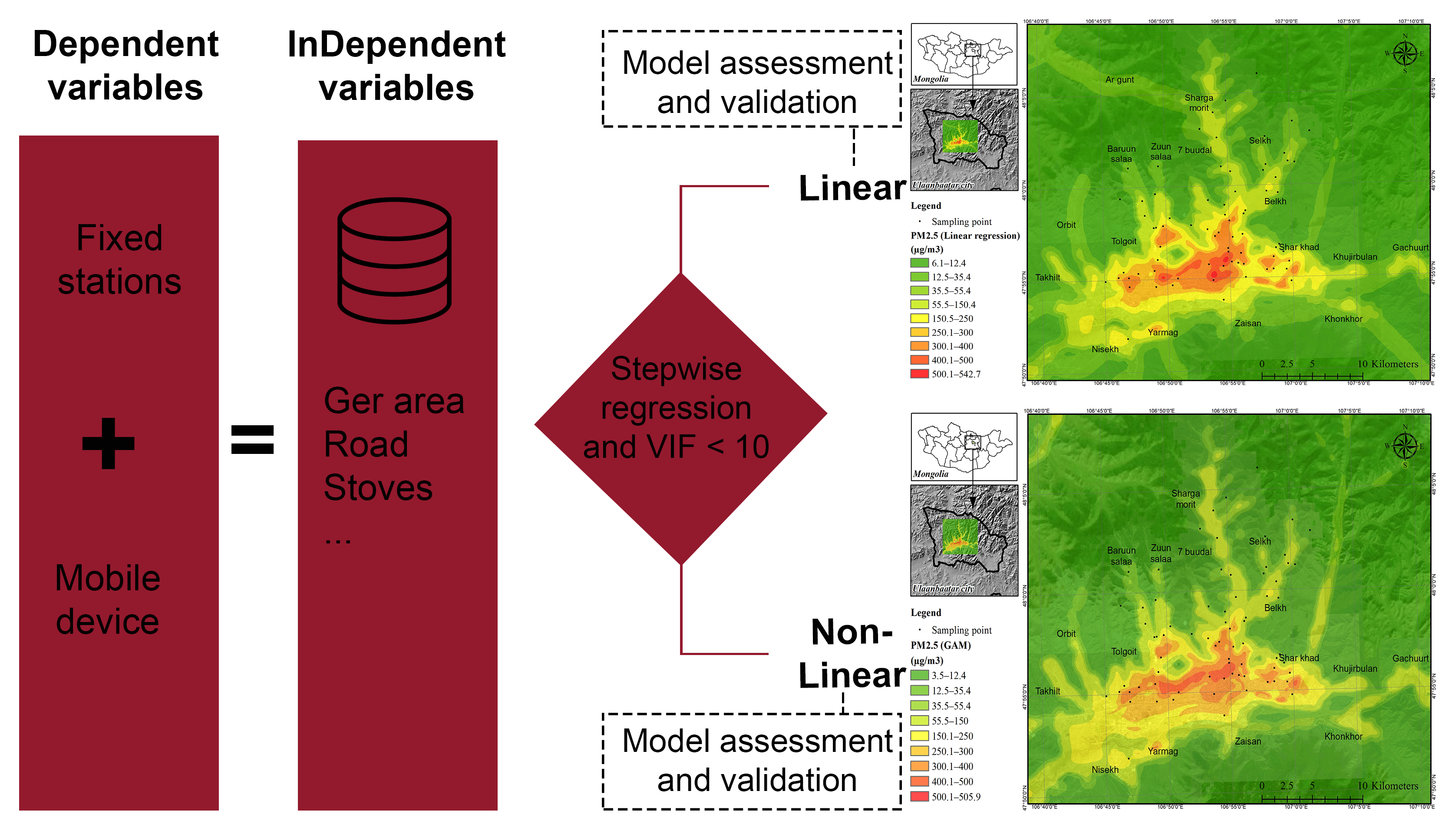
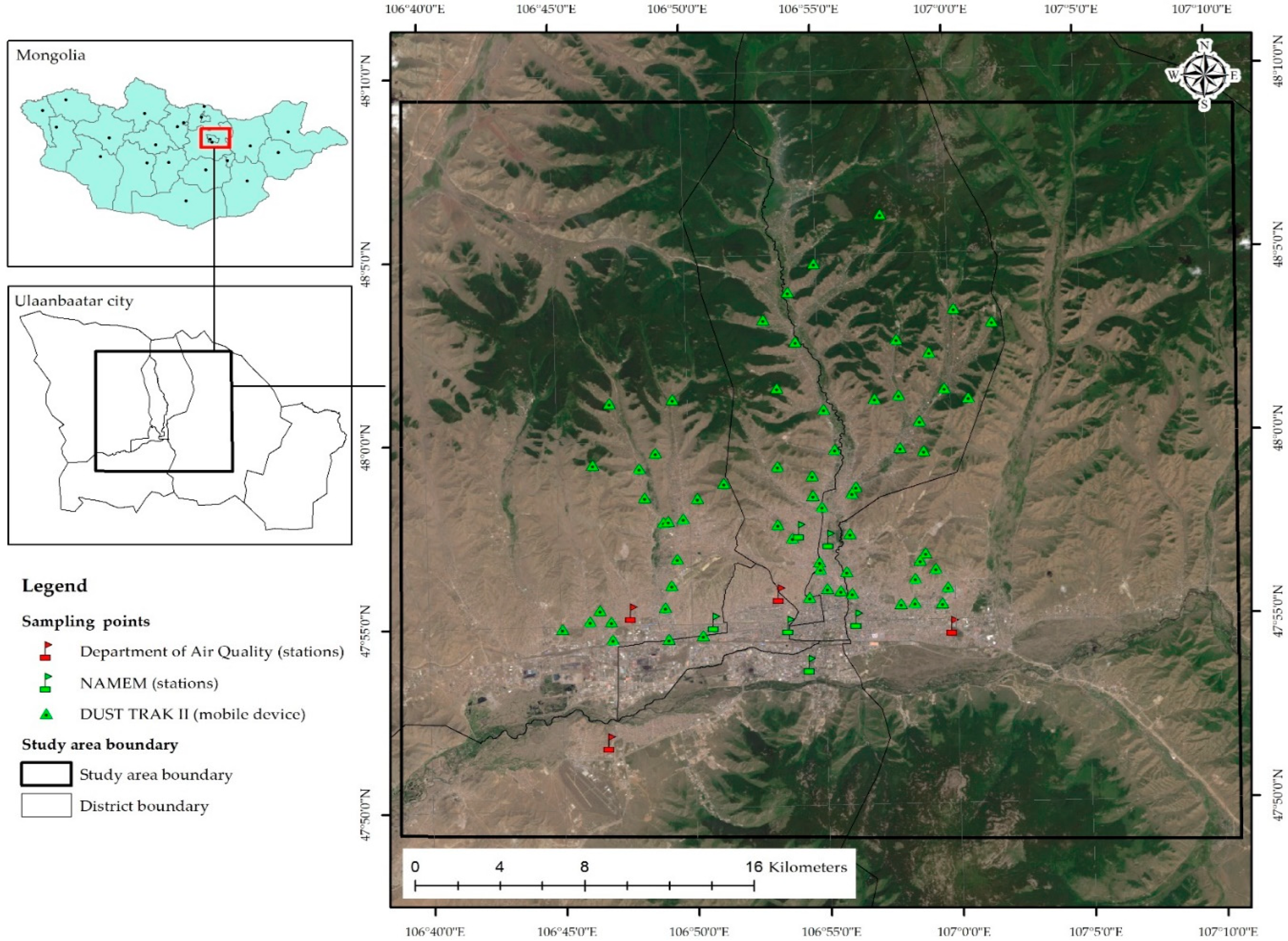
2.1. Study Area and Sampling

As mentioned above, Ulaanbaatar’s PM2.5 pollution is far too high early in the morning and in the evening, and this influences Ulaanbaatar citizens’ health. Thus, there is a need to map PM2.5 peak dispersion accurately and to understand the risk level of the air that we breathe in the morning and evening. Even though Ulaanbaatar’s air pollution is measured at 16 locations [24], until now, accurate dispersion mapping methods have not been developed due to the scarcity of monitoring stations, which means that air pollution dispersion is being mapped by dots. Of these stations, the Department of Capital City Air Quality possesses 5, and the other 11 belong to the National Agency of Meteorology and Environmental Monitoring (NAMEM). Some monitoring stations do not measure all pollutants, and only 10 stations measure the PM2.5 every 15 min–1 h.
The study area covers all residential areas of Ulaanbaatar, including the outskirts of the city, which amounts to 1464.95 square kilometers (37 km × 39.7 km) (Figure 1).
The ENVEA Environnement SA MP101 m Outdoor Air Quality Monitoring Station is a fully automated system for detecting the concentration of airborne particles. In the event that regulatory thresholds are exceeded, this device will sound an alarm. It can monitor particulate matter (PM10 and PM2.5) continuously. Furthermore, this gauge uses a beta-ray attenuation measurement approach. By measuring the amount of radiation absorbed by a sample collected on a fiber tape after being exposed to a radioactive source, the concentration of particulate matter can be calculated. According to the monitoring stations’ measurements on 17 January 2021 (Figure 2), Ulaanbaatar’s PM2.5 pollution reaches its minimum level in the afternoon, or from 02:00 pm to 05:00 pm. From 06:00 pm until the following morning, it increases continuously and reaches 400 μg/m3. However, these measurements are relatively low due to the stations being located in the city center, far from the ger area. Concentrations measured in the center are considerably lower than those measured in the ger area [20]. The ger area’s fine particulate matter pollution is around two times higher than the city center’s fine particulate matter pollution [25].
Based on other researchers’ experience [20,21,22,26], the “DUST TRAK II Aerosol Monitor 8532” mobile device was borrowed from the Department of Environment and Forest Engineering, National University of Mongolia, and was utilized for the field study. This portable device has a “Certificate of Calibration and Testing” (certificate serial number: 8532134301) and can measure aerosol concentrations for PM1, PM2.5, respirable, or PM10 size fractions with a corresponding impactor kit. It can also be used to evaluate the interior and outdoor air pollution. The major goal was to completely map the PM2.5 pollution in Ulaanbaatar. Sampling was done during the most polluted period of the day, 05:00–11:00 am and 06:00–00:00 pm, on Sunday 17 January 2021, mostly sampling the ger area region. Based on the work of Ryan et al. [20] and Grazio Fattoruso [27], this sample campaign took place over the course of a single day. In addition, the results of the measurements were compared with long-term measurements taken at fixed stations, and since the results of the measurements were found to be consistent with the long-term average measurements taken at fixed stations, the authors concluded that the data could be used to create LUR models. A total of 64 locations were sampled and a total of 74 locations’ samples (adding in 10 monitoring stations’ samples) were used as dependent variables for the LUR model. Fixed stations and mobile device measurements’ descriptive statistics are shown in Table 1.

2.2. Predictor Variables

The LUR model is based on the environmental characteristics of the study area, especially characteristics that influence the pollutant emission intensity and dispersion efficiency [28]. Thus, in this study, two types of predictor variables were collected, air pollution sources and the environmental characteristics that influence air pollution dispersion. The integration of road networks, traffic count information, topography, and land cover data within a geographic information system are common throughout all of these models [29]. According to these research results and conclusions, 22 independent variables (Table 1) that were related to Ulaanbaatar’s PM2.5 pollution were collected. The main sources of PM2.5 pollutant (gers and houses) were drawn from Google Earth, according to Weiran Yuchi et al.’s research [1].
Heat-only boiler data were taken from the Department of Air Quality, Ulaanbaatar, all types of road data were obtained from Open Street Maps [30], and ALOS PALSAR Digital Elevation Data were obtained from the Alaska Satellite Facility, US [31]. Landcover data were classified from SENTINEL 2 data. Even though Mongolia has landcover change data dating back 5 years [32], its classification is not sufficient at the city level, so Ulaanbaatar’s land surface was classified into 5 types generally. After collecting all data, one full model was built using all these data. However, the results did not show the true dispersion of PM2.5. Thus, in order to remove some statistically insignificant independent variables, the Variance Inflation Factor (Table 2) was calculated and the correlation between independent variables was detected. Within the results of these calculations, as for the Variance Inflation Factor, 1 < VIF < 10 levels are generally acceptable for the model [33], and if it is greater than 10, it may create multicollinearity. From these results, VIFs greater than 10 were removed and there was no significant multicollinearity that needed to be corrected [34]. Thus, to remove insignificant variables based on a statistical assessment, the stepwise selection (both forward and backward) method was used. Forward and backward selections are combined in stepwise selection. Researchers begin without any predictor factors and gradually introduce the most beneficial ones (as in forward stepwise selection). Then, we eliminate any predictor variables (such as backward stepwise selection) that no longer improve the model fit [35]. It was then analyzed using the statistical program R, which produced the final model.

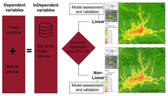
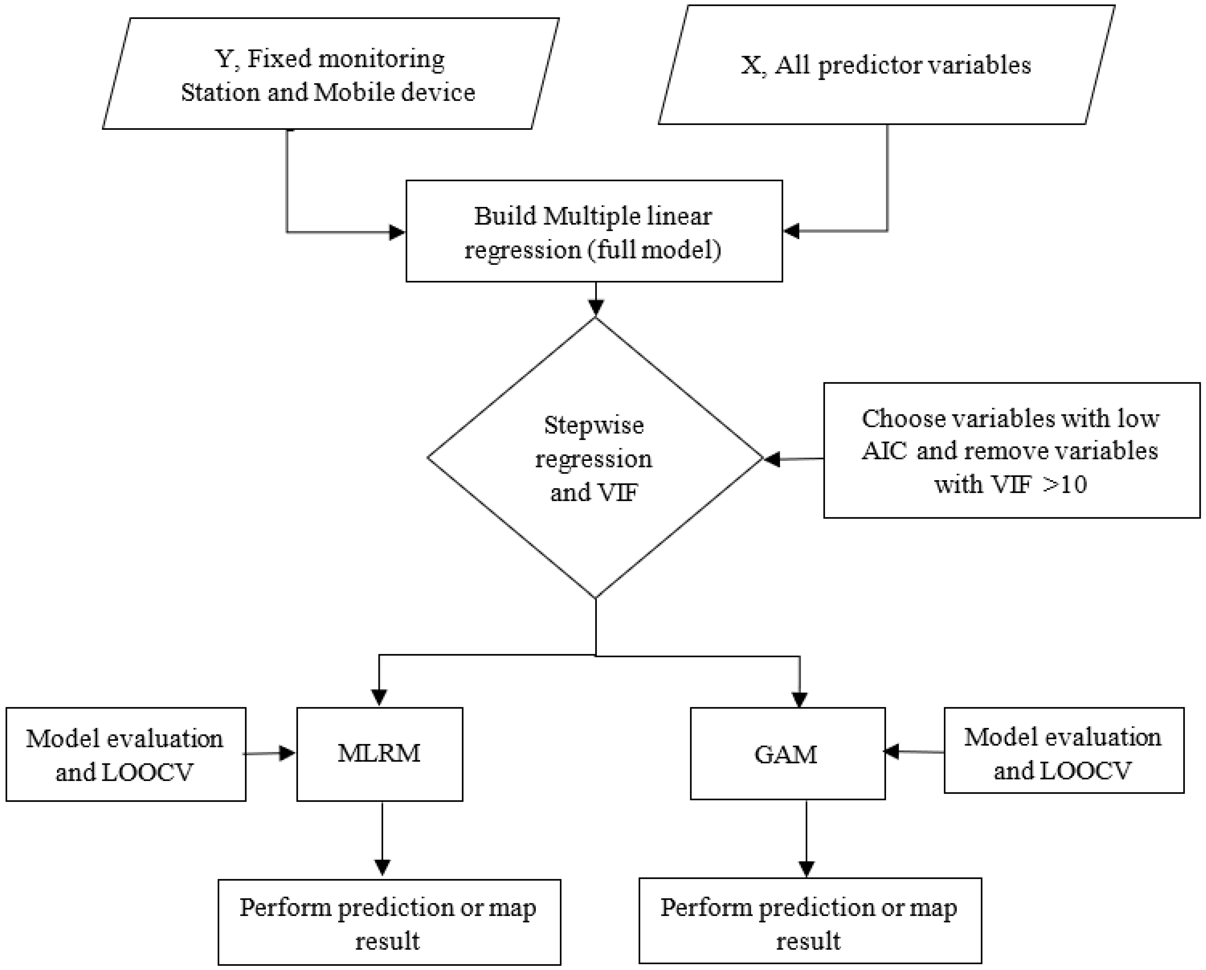
2.3. LUR Model Development

This research work aimed to map PM2.5 pollution during peak hours in Ulaanbaatar. According to the review study by Xing Zhe et al. [23], LUR modeling is the most popular model used in pollution estimation from mobile data and monitoring stations. LUR is based on the principle that pollutant concentrations at any location depend on the environmental characteristics of the surrounding area—particularly those that influence or reflect emission intensity and dispersion efficiency [36]. LUR models were originally developed to assess the exposure resulting from air pollution as a result of vehicular traffic, but they have since been expanded to cover air pollution epidemiology [37]. Recently, this model has been utilized widely, from city-level to continent-level air pollution [38,39,40,41].
The LUR model uses linear and nonlinear regression equations with measurement values (Y) and geographical predictor variables as independent variables (X). In this research, two LUR models were developed to model the spatial variability of PM2.5 concentrations and produce high-resolution maps with 100 m × 100 m resolution in Ulaanbaatar for the year 2019 (Figure 3).
The Multiple Linear Regression (MLR) equations were used as a linear regression model and the Generalized Additive Model (GAM) was used as a nonlinear multiple regression model. Linear regression models are easy to understand and interpret, used for inference, and allow the understanding of the linear relationship between the dependent and independent variables, but they can suffer from high bias. In other words, machine learning models such as “Gradient Boosting” and “Random Forest” are very useful in making predictions of complex relationships, but they tend to need huge amounts of data and are not easy to interpret. However, the GAM addresses this problem by fitting complex nonlinear relationships and making better predictions. Simultaneously, the GAM allows us to perform inferential statistics, and understand and explain the underlying structure of our used model [42]. As mentioned above in Section 2.2, the final LUR model’s independent variables were selected by the VIF and stepwise selection methods.
i. 
MLRM
PM2.5 ~ β0 + β1(House) + β2(Ger) + β3(MainPavedRoad) + β4(HeatOnlyBoilers) + β5(AgriculturalArea, 50 × 50 buffer) + ε
In Equation (1), β0 is the intercept; β1 to β5 are the β coefficients (slopes) of the independent variables; and ε is the residual (difference between predicted and observed values). β coefficients or slopes compare the strength of the effect of each individual independent variable to the dependent variable. The higher the absolute value of the β coefficient, the stronger the effect. This means that the variables can be easily compared to each other [43]. β coefficients are constant and these coefficients are found with the least square method.
ii. 
GAM
PM2.5 ~ α + s(House) + s(Ger) + s(MainPavedRoad) + s(HeatOnlyBoilers) + s(AgriculturalArea, 50 × 50 buffer) + ε
In Equation (2), α is the intercept; “s” is the smoothing function of the covariates; and ε is the error term or the residual. Smoothing functions are specified in a GAM formula using “s”, “te”, “ti”, and “t2” terms. In this study, the default “s” function has been used and it uses thin plate regression splines. These are low-rank isotropic smoothers of any number of covariates. Isotropic means that the rotation of the covariate coordinate system will not change the result of smoothing. “Low-rank” means that they have far fewer coefficients than there are data to smooth. They are reduced rank versions of the thin plate splines and use the thin plate spline penalty. They are the default smoothers for s terms because there is a defined sense in which they are the optimal smoother of any given basis dimension/rank [44].

2.4. Model Validation

In statistics, model validation tests the goodness of fit of the fitted model. Thus, in this part, we used the Leave-One-Out Cross-Validation technique with the R software on both the MRLM and GAM models. In total, 74 samples were used to build 74 models. Each model used 5 predictor variables. No pre-processing occurred and the resampling method was the Leave-One-Out Cross-Validation.

2.5. Mapping MLRM and GAM Model

In this research, two statistical and mapping software programs were used, generally ArcGIS 10.4 and R4.2.2. MRLM and GAM models were built and validated in the R statistical software with the “mgcv”, “MASS”, “ggplot2”, and “car” packages, etc. After building the MLRM and GAM models with R, all coefficients and prediction values were exported to the ArcGIS software and calculated with “field calculation”.
When spatially aggregated data are used, the modifiable areal unit problem (MAUP) is encountered. Thus, spatial grid points at different scale sizes, such as 100 m × 100 m, 200 m × 200 m, 500 m × 500 m, and 1 km × 1 km, were calculated in order to analyze MAUP sensitivity. There are many methods to perform analysis on MAUP, and spatial autocorrelation is one of them [45]. The Global Moran’s I spatial autocorrelation index is a widely used method to analyze MAUP, and, according to this index, for 100 m × 100 m scale aggregation, the Moran’s I index is 0.948, and it is the highest clustering index compared to other scale size experiments. In total, 146,211 points across the study region, with 100 m between each point, were used. It is convenient to use the interpolation approach to generate a surface map when working with a grid of equally spaced points because each point’s value may be extracted from the raster image as an individual value.
Models were then run using these point-independent values, making it possible to generate a high-resolution map using Equation (3).
Z p = i = 1 n ( z i d i p ) i = 1 n ( 1 d i p )
Z p = value to be estimated;
Z i = known value;
d i p = distance from the n data point to the power p of the point estimated.

3. Results

3.1. PM2.5 MLRM and GAM Models

Ulaanbaatar’s gers, houses, main paved roads, heat-only boilers, and agricultural land were used as independent variables in the final linear LUR model constructed using the stepwise selection results, with the dependent variable (Y) originating from PM2.5 measurements taken at fixed stations and mobile devices. The final linear model was defined as follows:
Y = 1.33259 + 15.85699 * ger + 5.28564 * b a i s h i n + 0.23285 * r _ m _ p + 2.00580 * stoves + 0.04753 * F 50 _ agri
Table 3 shows detailed information about the MLRM model, including the constant coefficients, standard error, t-value, p-value, and Variance Inflation Factor. The standard error of all independent values ranged between 0.006 and 4.02, and the same was true for the beta coefficient. The t-value was also between 0.117 and 6.953, or far from “0”, and we could thus reject the null hypothesis and prove that there were relationships between the dependent and independent variables. As for the p-value (Pr(>|t|)), gers, main paved roads, and agricultural land have high significance, while other independent values offer insufficient evidence against the null hypothesis. Moreover, all VIF coefficients are less than 5, meaning that there is no high correlation between the independent variables.
After building the MLRM model, all independent variables were also utilized for the nonlinear regression GAM. The effective degrees of freedom (edf) estimated from the GAM model were used as a proxy for the degree of nonlinearity in stressor–response relationships. According to Table 3, the edfs of independent variables such as houses, main paved roads, and heat-only boilers are equal to 1 and they have a linear relationship; for other independent variables, such as gers and agricultural land, the edfs are more than 2 and this indicates that they have a highly nonlinear relationship [46]. The p-value shows the significance level of independent variables. Gers and agricultural land’s values are less than 0.05, or they have significance, while others are more than 0.05, or they offer insufficient evidence against the null hypothesis (Table 4).

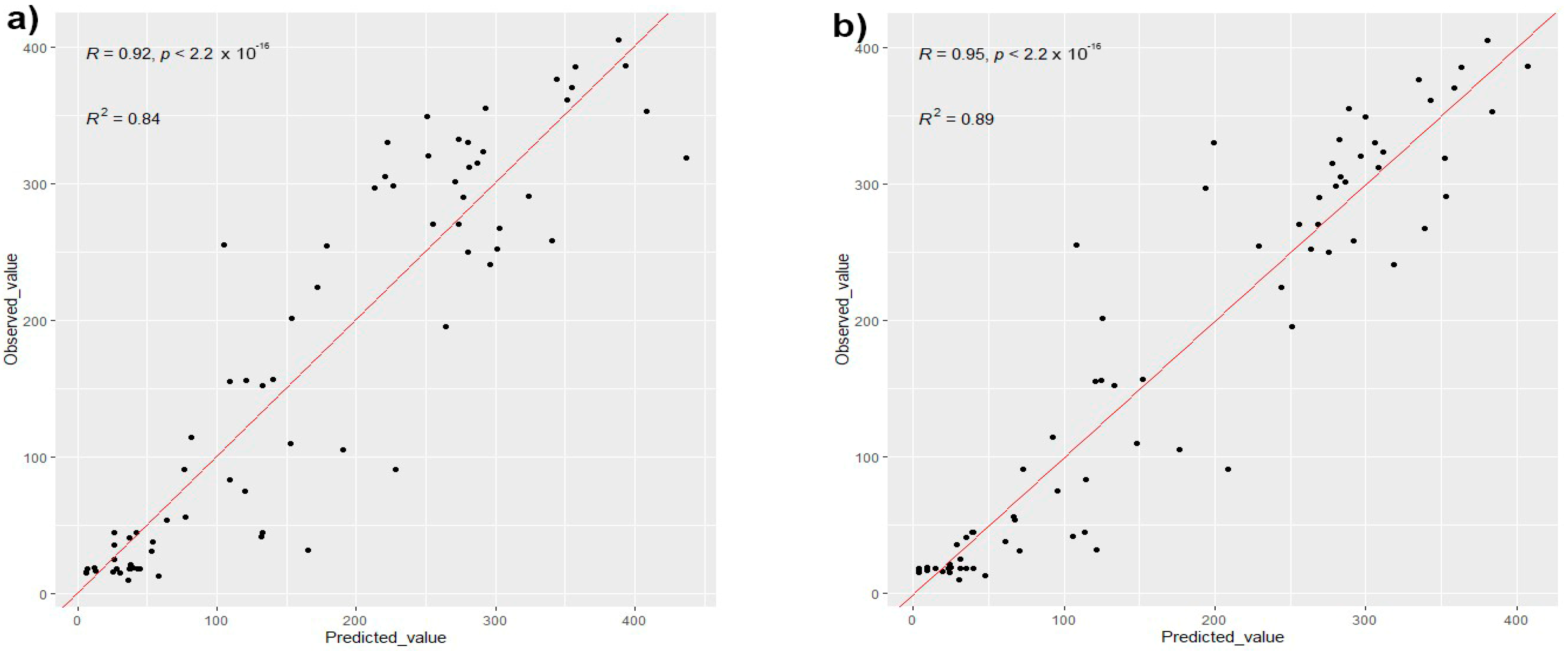
3.2. Model Accuracy and Validation
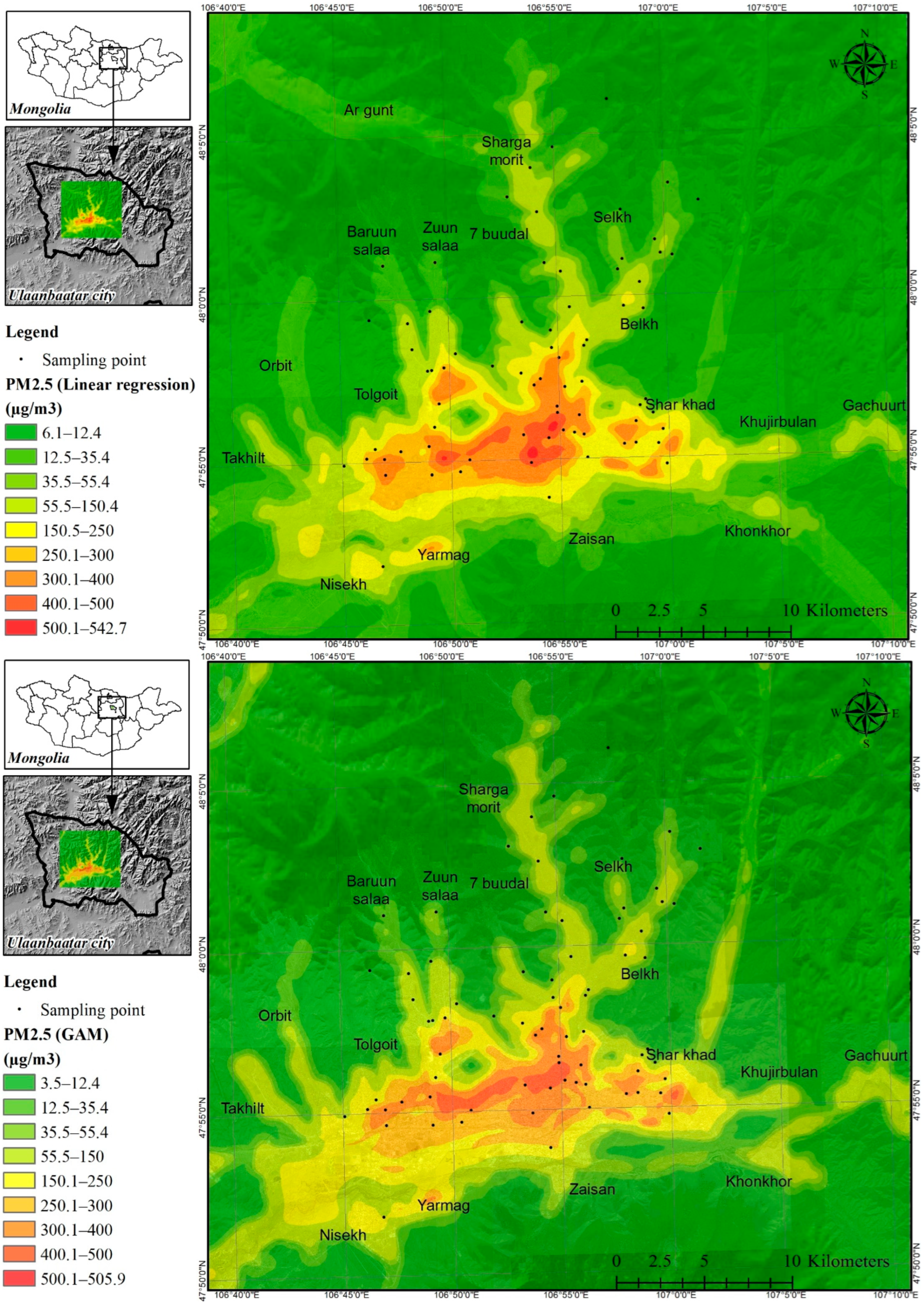
Several statistical metrics were calculated for the model assessment for both models (MLRM and GAM) and LOOCV. Statistical metrics used in this study were the determination coefficient (R2), root mean square error (RMSE), adjusted R2, and mean absolute error (MAE), which are widely used for model assessment. Figure 4 and Table 5 (LOOCV column) present the plots of the predicted and observed values, model accuracy, and LOOCV validation coefficients. As for the accuracy of the MLRM model, determination coefficient R2 = 0.84, adjusted R2 = 0.83, and RMSE = 53.25 μg/m3, and p-values were less than the significance level. As for the accuracy of the GAM model, the accuracy was slightly higher than that of the MLRM, or R2 = 0.89, adjusted R2 = 0.87, and RMSE = 44 μg/m3. The p-values of these models were 2 × 10⁻¹⁶ or much less than the significance level of 0.05, and the null hypothesis was rejected. Based on these assessment coefficients, the MLRM and GAM models predict reasonably well.
As for model validation, validation technique LOOCV was used and its accuracy coefficients were similar to the model fit assessment coefficients (Table 4): MLRM LOOCV determination coefficient R2 = 0.83, RMSE = 55.6 μg/m3, and MAE = 38.7 μg/m3; GAM LOOCV determination coefficient R2 = 65.5 μg/m3, RMSE = 65.5 μg/m3, and MAE = 47.7 μg/m3. Furthermore, there was no large difference or error between the fit model and LOOCV model.

3.3. Mapping

The MLRM and GAM models were run on each point within 146,211 grid points, with 100 m distances between them. Values of each point were interpolated with the Inverse Distance Weighting (IDW) method (Formula (3)), and a surface map was created (Figure 5). These maps depict the amount of PM2.5 pollution on 17 January 2021, one of the coldest days of the winter season. In other words, during the winter months, when most people stay at home and burn coal to heat their homes, for the peak hours of the day, such as early in the morning and late at night, there are significant levels of air pollution. In order to show exposure to PM2.5, the EPA’s Air Quality Index for 24-h Fine Particle Pollution Levels [47] was used for the legend. According to its categories, 0–12 μg/m3—“good”, 12.1–35.4 μg/m3—“moderate”, 35.5–55.4 μg/m3—“unhealthy for sensitive people”, 55–150.4 μg/m3—“unhealthy”, 150.5–250.4 μg/m3—“very unhealthy”, <250.5 μg/m3 —hazardous. From this, Ulaanbaatar’s PM2.5 pollution exceeds the hazardous level and this situation continues for nearly every half day in the winter months. Additionally, Ulaanbaatar’s topography, being surrounded by mountains, blocks air movement and increases the accumulation of pollution throughout the city.
Finally, the PM2.5 dispersion maps show a spatial dispersion intensity in Ulaanbaatar City similar to the results of Yukimasa et al. [12], Ryan W.Allen et al. [1], and the “Project to strengthen air pollution control capacity in Ulaanbaatar, Mongolia” (PSAPCCU) report [48]. Yukimasa et al. used the diffusion simulation method, but its results show the total emissions of 6 full hours of combustion with each stove’s particulate matter emission capability. Ryan W. Allen et al. used the LUR model, but they showed the spatial variability of the annual average PM2.5 concentration and did not report model prediction errors. The PSAPCCU mapped air pollution dispersion with the CALMET + CALPUFF model. Its spatial variability was determined as grid cells, and compared to this research, it is inaccurate. We did not find similar research using LUR modeling for PM2.5 over Ulaanbaatar City. The abovementioned results, despite using different methods, show similar spatial variability in the dispersion result. The main advantage of this study’s results compared to previous studies is more detail and wider coverage of the residential areas of Ulaanbaatar.

4. Discussion

A few studies have attempted to model particulate matter pollution exposure at the city level in Ulaanbaatar [1,4,12,21,22]. However, the resulting maps are not highly detailed and are not very clear. Weiran Yuchi et al. [1] tried to map air pollution dispersion with the LUR model using independent variables such as wetness, greenness, gers, and road lengths. However, they did not create a map, showing only the independent variable dispersion map. According to their results, independent variables explained an average of 70% of the model. This research could not issue a satisfactory result. Sarath Guttikunda et al. [4,49] mapped air pollution with the ATMOS model, but their results’ spatial variability was not accurate. Yukimasa et al. [12] and Ryan W et al. [20] also tried to map air pollution with statistical data, and their result regarding spatial variability was similar to the results of this study, but their spatial accuracy was too poor. In recent years, the Department of Capital City Air Quality has measured particulate matter, but its stations are mainly located downtown, and measurement results are issued on the website with dot marks. Thus, the accurate modeling of particulate matter pollution is still a priority issue in Ulaanbaatar.
In this research, data relevant to Ulaanbaatar’s PM2.5 pollution were collected as independent variables for the LUR model. Many of them were not well suited to the LUR model due to the characterization of Ulaanbaatar’s air pollution sources. For instance, many researchers who have developed a LUR model used altitude or a Digital Elevation Model (DEM) as an independent variable. This contrasts with Ulaanbaatar’s ger area, which is the main source of PM2.5, being mainly located on the tops of mountains. If a DEM was used in this LUR model, it would show an incorrect prediction suggesting that areas with higher elevation have high pollution. Thus, DEM data are not useful for the Ulaanbaatar LUR model because they would show that higher places have more pollution and the residential areas located in lower places have less pollution.
Another finding was that many researchers use population density data for an LUR model based on the principle that higher population density leads to higher air pollution. This is contrary to Ulaanbaatar, where ger area residents mainly live in one-floor houses or “ger” dwellings as a single family within a fenced area of around 0.07 hectares. Apartment residents live in multi-floored apartments, having many families in a small area. In other words, in the ger area, every single family emits PM2.5 pollution through a chimney when burning coal, and apartment-residing families do not, since they are connected to the central heating system. This would show an incorrect prediction that low-population-density areas generate high pollution. Thus, population density data are also not useful for the Ulaanbaatar LUR model.
European researchers mostly use CORINE land cover monitoring data [50] for an LUR model. This integrated land cover database shows integrated results for LUR model development. As for Ulaanbaatar, there are no land cover monitoring data at the city scale. Thus, in this study, the researchers classified land cover themselves, and this will likely result in different study results as compared with other similar studies. Even though Mongolia has land cover monitoring data at 5-year intervals, they are not suitable at the scale needed for the analysis of the city. There is a requirement to monitor city-level land cover change, as with CORINE land cover data. This type of data will be fundamental, resulting in integrated data not only for air pollution studies but also various other environmental studies. Consequently, in this study, only agricultural land cover data were utilized for the model as an independent variable.
Ulaanbaatar is situated in the Tuul river valley, surrounded by high mountains. This topographic condition is the main factor in blocking air movement and increasing the accumulation of air pollution [51]. Additionally, this is one factor that creates “an inversion layer” over the city. This inversion layer appears as black smoke clouds over the city, and the accumulated clouds easily differ from cleaner air. When PM2.5 was sampled at the top of the mountains, the city appeared as if it was diving into smoke. This characteristic was detected in the resulting image of this study from the drastically differentiated PM2.5 levels in the mountain slope regions.
This research’s main findings include the more detailed spatial variability of PM2.5 pollution and greater coverage of the residential areas of Ulaanbaatar City compared to previous studies. In addition, the results of this research were evaluated with some statistical methods, and the evaluation coefficients were reasonably high. This research’s results are very accurate and can have very practical uses. For instance, the Mongolian government is planning to build “micro centers”, which are infrastructures that aim to address the most polluted “ger” areas within the scope of the National Program to Decrease Air and Environmental Pollution [52]. These “micro centers” are planned to include 200–300 householders and will be provided with a heating system. It is hoped that this research can offer a recommendation in choosing where to build “micro centers” in the ger area.

Limitations

Our LUR models combined the data from a mobile device and a fixed station into a single model due to the fact that there were only 10 fixed stations, the majority of which were downtown. These measurement data could not cover all residential areas, and thus we could not build the models properly. Thus, there is a need to measure air pollution on the outskirts of the city or in the ger area. We borrowed a DUST TRAK II mobile device for PM2.5 measurement from the Department of Environment and Forest Engineering, National University of Mongolia, and performed a short-term sampling campaign with this device based on the experience of Ryan et al. [20] and Grazio Fattoruso [27]. In our study, in order to show the highest pollution concentration, measurement was conducted early in the morning and in the evening. Thus, it is impossible to compare this result with daytime air pollution.
Our model might be constrained by the availability of predictor data. Gers, homes, and heat-only boilers in Ulaanbaatar are the main sources of PM2.5 pollution, since they employ coal combustion stoves. Even though heat-only boilers and gers and houses are the leading sources of PM2.5 pollution in Ulaanbaatar, the Department of Capital City Air Quality only keeps track of heat-only boiler statistics. Since gers and houses on the outskirts of the city must be included in models as the primary source of PM2.5 pollution, the authors made the decision to collect data from Google Maps in response to the study by Weiran Yu Chi et al. Google Maps data, on the other hand, remained largely stable over the course of the three years, indicating that the final two models are largely accurate in reflecting the spatial variability in PM2.5 pollution throughout the year 2021.

5. Conclusions

The aim of this study was to show the highest PM2.5 pollution dispersion in Ulaanbaatar by measuring pollution during peak hours, and to detect the most polluted areas of the city. The linear (MLRM) and nonlinear (GAM) LUR models, a widely used approach to assess exposure to air pollution, were used as the primary method for dispersion mapping and their performance was high, with MLRM R2 = 0.84, adjusted R2 = 0.83, RMSE = 53.25 µg/m3, and GAM R2 = 0.89, adjusted R2 = 0.87, RMSE = 44 µg/m3. In order to validate the models, the LOOCV technique was run on both MLRM and GAM. Their performance were again high, with MRLM LOOCV R2 = 0.83, RMSE = 55.6 µg/m3, MAE = 38.7 µg/m3, and GAM LOOCV R2 = 0.77, RMSE = 65.5 µg/m3, MAE = 47.7 µg/m3. From these results, GAM works better than MRLM or its fit model, and the LOOCV assessment coefficients are higher than those for the MRLM fit model and LOOCV.
Sources contributing to PM2.5 were dominated by emissions from coal combustion in the ger area. Most householders in the ger area use coal-burning stoves as a home heating device. Furthermore, due to heating of the home and cooking, both in the morning and evening, PM2.5 pollution increases heavily, and exceeds the “hazardous” level. According to this study’s results, Ulaanbaatar’s PM2.5 pollution reaches over 500 μg/m3. This occurs mainly in the city center during the winter, early in the morning, and in the evening, continuing for around half a day. In addition to excessive smoke emissions, the topography of the capital city plays a significant role. In the Tuul river valley, surrounded by mountains, an inversion layer is created, normal air mixing ceases, and pollutants are trapped in the lower layer. As a result of this, PM2.5 pollution accumulates significantly, especially on calm days, where it can be 2–3 times higher than the hazardous level.
With such high fine particulate matter concentrations, there are likely to be significant health implications for Ulaanbaatar’s citizens. Based on the findings of this study, stoves used for heating are the primary cause of PM2.5 pollution. Therefore, there is a need to switch from stoves to various fuel-free heating options. In other words, the ger region needs to adopt electrical heating gadgets or a central heating system. This will reduce PM2.5 pollution more successfully. Additionally, the resulting map shows the intensity of the level of air pollution, and people should avoid living in and visiting areas with high levels of pollution.
During the experimentation phase of model construction, our LUR models revealed that altitude and population density data are not always adequate due to PM2.5 pollution source dispersion, which is a theoretical contribution to the LUR model. The ger district of Ulaanbaatar, the city’s primary contributor to PM2.5 pollution, is located in relatively remote, high-altitude areas; its population is dispersed sparsely compared to the downtown, densely populated, central district. In contrast, according to the laws of physics, particulate matter pollution must build up in lower places, and places with a large number of people must support it heavily. In Ulaanbaatar, caused by particulate matter pollution source dispersion, this pattern is the opposite.
Finally, these maps illustrate the extent to which air pollution is a problem and how much of a geographic area is affected. We anticipate that these data will be useful in helping decision-makers to identify areas where urgent action is required to reduce air pollution.

Author Contributions

Conceptualization, X.-Y.Y. and O.E.; methodology, O.E.; software, O.E.; validation, O.E.; formal analysis, O.E.; investigation, O.E.; resources, O.E.; data curation, O.E.; writing—original draft preparation, J.C.; writing—review and editing, M.L.; visualization, O.E.; supervision, X.-Y.Y.; project administration, O.E.; funding acquisition, M.L. All authors have read and agreed to the published version of the manuscript.

Funding

This research was funded by a National Research Foundation of Korea (NRF) grant provided by the Ministry of Education (No. 2021R1I1A1A01060652).

Acknowledgments

We wish to thank Chonokhuu Sonomdagva (Department of Environment and Forest Engineering, National University of Mongolia), who lent us the expensive “DUST TRAK II” mobile device for the field research. We also thank Ganbaatar Ochirbat, and researchers at the Divisio/n of Innovation Technology, Institute of Physical Technology, MAS, who spent a full day with us and helped to sample the PM2.5 for field measurement. With their help, the field measurement was performed effectively and efficiently, and this provided the most significant data for this research work.

Conflicts of Interest

The authors declare no conflict of interest.

References

  1. Yuchi, W.; Knudby, A.; Cowper, J.; Gombojav, E.; Amram, O.; Walker, B.B.; Allen, R.W. A description of methods for deriving air pollution land use regression model predictor variables from remote sensing data in Ulaanbaatar, Mongolia. Can. Geogr. 2016, 60, 333–345. [Google Scholar] [CrossRef]
  2. New Yourk State. February 2018. Available online: https://www.health.ny.gov/environmental/indoors/air/pmq_a.htm#:~:text=Exposure%20to%20fine%20particles%20can,as%20asthma%20and%20heart%20disease (accessed on 19 February 2023).
  3. HEI International Scientific Oversight Committee. Outdoor Air Pollution and Health in the Developing Countries of Asia: A Comprehensive Review; Health Effects Institute: Boston, MA, USA, 2010. [Google Scholar]
  4. Guttikunda, S.K.; Lodoysamba, S.; Bulgansaikhan, B.; Dashdondog, B. Particulate pollution in Ulaanbaatar, Mongolia. Air Qual. Atmos Health 2013, 6, 589–601. [Google Scholar] [CrossRef]
  5. World Health Organization. Available online: https://www.who.int/health-topics/air-pollution#tab=tab_1 (accessed on 19 February 2023).
  6. Warburton, D.; Warburton, N.; Wigfall, C.; Chimedsuren, O.; Lodoisamba, D.; Lodoysamba, S.; Jargalsaikhan, B. Impact of Seasonal Winter Air Pollution on Health across the Lifespan in Mongolia and Some Putative Solutions. Ann. Am. Thorac. Soc. 2018, 15, S86–S90. [Google Scholar] [CrossRef] [PubMed]
  7. National Statistics Office. Census 2020. Ulaanbaatar. 2020. Available online: https://www.1212.mn/mn/statistic/statcate/573051/table-view/DT_NSO_0300_071V3 (accessed on 19 February 2023).
  8. Үндэсний статистикийн хoрoo. Icon News, Мoнгoл Улсын нийт өрхийн 70% нь галлагаатай сууцанд амьдарч байна. 2019. Available online: https://ikon.mn/n/1hus (accessed on 19 February 2023).
  9. Агаарын чанарын алба. Агаарын чанар. Available online: http://agaar.mn/static/stove-distribution (accessed on 28 January 2022).
  10. World Air Quality Report 2020; IQAir: Goldach, Switzerland, 2021.
  11. IQAir. Air Quality and Pollution City Ranking. 31 January 2022. Available online: https://www.iqair.com/world-air-quality-ranking (accessed on 31 January 2022).
  12. Takemoto, Y.; Takahashi, M.; Awaya, K.; Ito, K.; Takeuchi, S. Numerical Simulation of Air Pollution in Ulaanbaatar City, Mongolia. J. Mater. Sci. Eng. B 2015, 5, 187–195. [Google Scholar] [CrossRef] [Green Version]
  13. Агаарын чанарын алба. Агаарын чанар. 24 January 2022. Available online: http://agaar.mn/files/article/1066/2022.01.17-2022.01.23%20%20(23).pdf (accessed on 28 January 2022).
  14. Стандарт хэмжилзүйн газар. Мoнгoл улсын стандарт. 8 July 2016. Available online: https://estandard.gov.mn/standard/reader/3377#0-yoimswmqdpgvqlgb.jpg (accessed on 28 January 2022).
  15. WHO. Ambient (Outdoor) Air Pollution. 22 September 2021. Available online: https://www.who.int/news-room/fact-sheets/detail/ambient-(outdoor)-air-quality-and-health (accessed on 28 January 2022).
  16. The World Air Quality Project. Air Pollution: Real-Time Air Quality Index. Available online: https://aqicn.org/city/ulaanbaatar/mnb/ (accessed on 29 January 2022).
  17. Нoгooн хөтөч. Агаарын бoхирдoл. Available online: http://www.nogoonhutuch.mn/p/c/19/lastOne (accessed on 31 January 2022).
  18. Үндэсний Статистикийн Хoрoo. Улаанбаатар хoтын гадаад oрчны агаарын бoхирдoл ба эрүүл мэнд. Улаанбаатар. 2019. Available online: https://www2.1212.mn/BookLibraryDownload.ashx?url=UB_health_airpolution_2019.pdf&ln=Mn (accessed on 19 February 2023).
  19. Үндэсний Статистикийн Хoрoo, Эрүүл мэнд хөгжлийн төв. Улаанбаатар хoтын агаарын бoхирдлын хүний эрүүл мэндэд үзүүлэх нөлөө. Улаанбаатар хoт. 2020. Available online: https://www.unicef.org/mongolia/media/911/file/Agaariin_bohirdol_report_mn.pdf (accessed on 19 February 2023).
  20. Allen, R.W.; Gombojav, E.; Barkhasragchaa, B.; Byambaa, T.; Lkhasuren, O.; Amram, O.; Takaro, T.K.; Janes, C.R. An assessment of air pollution and its attributable mortality in Ulaanbaatar, Mongolia. Air Qual. Atmosphere Health 2011, 6, 137–150. [Google Scholar] [CrossRef] [PubMed] [Green Version]
  21. Minet, L.; Gehr, R.; Hatzopoulou, M. Capturing the sensitivity of land-use regression models to short-term mobile monitoring campaigns using air pollution micro-sensors. Environ. Pollut. 2017, 230, 280–290. [Google Scholar] [CrossRef] [PubMed]
  22. Lim, C.C.; Kim, H.; Vilcassim, M.R.; Thurston, G.D.; Gordon, T.; Chen, L.C.; Lee, K.; Heimbinder, M.; Kim, S.Y. Mapping urban air quality using mobile sampling with low-cost sensors and machine learning in Seoul, South Korea. Env. Int. 2019, 131, 105022. [Google Scholar] [CrossRef] [PubMed]
  23. Xie, X.; Semanjski, I.; Gautama, S.; Tsiligianni, E.; Deligiannis, N.; Rajan, R.T.; Pasveer, F.; Philips, W. A Review of Urban Air Pollution Monitoring and Exposure Assessment Methods. ISPRS Int. J. Geo-Inf. 2017, 6, 389. [Google Scholar] [CrossRef] [Green Version]
  24. Clean Air Foundation. Air Pollution Monitoring Station Live. Available online: http://agaar.mn/index (accessed on 31 January 2022).
  25. Enkhtsolmon, O.; Matsumoto, T.; Tseveen, E. Cost Benefit Analysis of Air Pollution Abatement Options in the Ger Area, Ulaanbaatar, and Health Benefits Using Contingent Valuation. Int. J. Environ. Sci. Dev. 2016, 7, 330. [Google Scholar] [CrossRef] [Green Version]
  26. Hankey, S.; Sforza, P.; Pierson, M. Using Mobile Monitoring to Develop Hourly Empirical Models of Particulate Air Pollution in a Rural Appalachian Community. Environ. Sci. Technol. 2019, 53, 4305–4315. [Google Scholar] [CrossRef] [PubMed]
  27. Fattoruso, G.; Toscano, D.; Cornelio, A.; De Vito, S.; Murena, F.; Fabbricino, M.; Di Francia, G. Using Mobile Monitoring and Atmospheric Dispersion Modeling for Capturing High Spatial Air Pollutant Variability in Cities. Atmosphere 2022, 13, 1933. [Google Scholar] [CrossRef]
  28. Wikipedia. Land Use Regression Model. Available online: https://en.wikipedia.org/wiki/Land_use_regression_model (accessed on 19 February 2023).
  29. Ryan, P.H.; Lemasters, G.K. A Review of Land-use Regression Models for Characterizing Intraurban Air Pollution Exposure. Inhal. Toxicol. 2007, 19 (Suppl. S1), 127–133. [Google Scholar] [CrossRef] [PubMed] [Green Version]
  30. Christopher, M. Free, Mongolia GIS Data. Rutgers University. Available online: https://marine.rutgers.edu/~cfree/gis-data/mongolia-gis-data/ (accessed on 19 February 2023).
  31. Earth Data. ALOS PALSAR. Available online: https://asf.alaska.edu/data-sets/sar-data-sets/alos-palsar/ (accessed on 19 February 2023).
  32. Байгаль oрчны мэдээллийн сан. Газар. Available online: https://www.eic.mn/land/gis.php (accessed on 19 February 2023).
  33. How2stats, Variance Inflation Factor (VIF). Available online: http://www.how2stats.net/2011/09/variance-inflation-factor-vif.html (accessed on 5 February 2022).
  34. Investopedia Team. Variance Inflation Factor, Investopedia, 12 February 2023. Available online: https://www.investopedia.com/terms/v/variance-inflation-factor.asp#:~:text=In%20general%20terms%2C,variables%20are%20highly%20correlated2 (accessed on 19 February 2023).
  35. Statistical Tools for High-throughput Data Analysis. Model Selection Essentials in R. 11 March 2018. Available online: http://www.sthda.com/english/articles/37-model-selection-essentials-in-r/154-stepwise-regression-essentials-in-r/#:~:text=The%20stepwise%20regression%20(or%20stepwise,model%20that%20lowers%20prediction%20error (accessed on 19 February 2023).
  36. Integrated Environmental Health Impact Assessment System. Land Use Regression in IEHIAS. Opasnet, 13 October 2014. Available online: http://en.opasnet.org/w/Land_use_regression_in_IEHIAS (accessed on 19 February 2023).
  37. Allen, R. Wikipedia. 26 November 2018. Available online: https://en.wikipedia.org/wiki/Land_use_regression_model#:~:text=A%20land%20use%20regression%20model,particularly%20in%20densely%20populated%20areas.&text=This%20results%20in%20an%20equation,predictor%20variables%20in%20specific%20locations (accessed on 19 February 2023).
  38. Lee, M.; Brauer, M.; Wong, P.; Tang, R.; Tsui, T.H.; Choi, C.; Cheng, W.; Lai, P.-C.; Tian, L.; Thach, T.-Q.; et al. Land use regression modelling of air pollution in high density high rise cities: A case study in Hong Kong. Sci. Total Environ. 2017, 592, 306–315. [Google Scholar] [CrossRef] [PubMed] [Green Version]
  39. Gulliver, J.; de Hoogh, K.; Hoek, G.; Vienneau, D.; Fecht, D.; Hansell, A. Back-extrapolated and year-specific NO2 land use regression models for Great Britain—Do they yield different exposure assessment? Environ. Int. 2016, 92–93, 202–209. [Google Scholar] [CrossRef] [PubMed] [Green Version]
  40. Naughton, O.; Donnelly, A.; Nolan, P.; Pilla, F.; Misstear, B.; Broderick, B. A land use regression model for explaining spatial variation in air pollution levels using a wind sector based approach. Sci. Total Environ. 2018, 630, 1324–1334. [Google Scholar] [CrossRef] [PubMed] [Green Version]
  41. Vienneau, D.; de Hoogh, K.; Beelen, R.; Fischer, P.; Hoek, G.; Briggs, D. Comparison of land-use regression models between Great Britain and the Netherlands. Atmos. Environ. 2010, 44, 688–696. [Google Scholar] [CrossRef]
  42. Anello, E. Generalized Additive Models with R. Available online: https://pub.towardsai.net/generalized-additive-models-with-r-5f01c8e52089 (accessed on 4 January 2023).
  43. Glen, S. Statistics How to. Available online: https://www.statisticshowto.com/standardized-beta-coefficient/ (accessed on 4 January 2023).
  44. Wood, S. ETH Zurich, Department of Mathematics. Available online: https://stat.ethz.ch/R-manual/R-devel/library/mgcv/html/smooth.terms.html (accessed on 1 January 2023).
  45. Grasland, C.; Madelin, M.; Mathian, H. The Modifiable Areas Unit Problem (Final Report); ESPON Coordination Unit: Luxembourg, 2022. [Google Scholar]
  46. Hunsicker, M.E.; Kappel, C.V.; Selkoe, K.A.; Halpern, B.S.; Scarborough, C.; Mease, L.; Amrhein, A. Characterizing driver-response relationships in marine pelagic ecosystems for improved ocean management. Ecol. Appl. 2016, 26, 651–663. [Google Scholar] [CrossRef] [PubMed]
  47. United States Environmental Protection Agency. Clean Air Fairbanks. 2013. Available online: https://cleanairfairbanks.files.wordpress.com/2013/01/aqi-chart-for-pm-2-5-pollution-2013.pdf (accessed on 19 February 2023).
  48. Агаарын бoхирдлыг бууруулах газар. Мoнгoл улс Улаанбаатар хoтын Aгаарын бoхирдлын хяналтын чадавхыг бэхжүүлэх төсөл (2-р үе шат). Улаанбаатар. 2017. Available online: https://openjicareport.jica.go.jp/pdf/12289310.pdf (accessed on 20 February 2023).
  49. Guttikunda, S. Urban Air Pollution Analysis in Ulaanbaatar, Mongolia. Ulaanbaatar. 2008. Available online: https://urbanemissions.info/wp-content/uploads/docs/SIM-05-2008.pdf (accessed on 19 February 2023).
  50. Land Monitoring Service. Copernicus. Available online: https://land.copernicus.eu/pan-european/corine-land-cover (accessed on 19 February 2023).
  51. Amarsaikhan, D.; Battsengel, V.; Nergui, B.; Ganzorig, M.; Bolor, G. A Study on Air Pollution in Ulaanbaatar City, Mongolia. J. Geosci. Environ. Prot. 2014, 2, 123. [Google Scholar] [CrossRef]
  52. БОАЖ яамны сайд. АГААР, ОРЧНЫ БОХИРДЛЫГ БУУРУУЛАХ ҮНДЭСНИЙ ХӨТӨЛБӨРИЙГ ХЭРЭГЖҮҮЛЭХ АРГА ХЭМЖЭЭНИЙ ТӨЛӨВЛӨГӨӨ. 2017. Available online: http://www.agaar.mn/files/article/580/Agaar,%20orchnii%20bohirdliig%20buuruulah%20undesnii%20hutulburiin%20plan.pdf (accessed on 19 February 2023).
Figure 1. Study area and sampling points.
Remotesensing 15 01174 g001
Figure 2. PM2.5 concentration levels during a day.
Remotesensing 15 01174 g002
Figure 3. LUR model development flow chart.
Remotesensing 15 01174 g003
Figure 4. Observed and predicted value relationship for the (a) MLRM and (b) GAM.
Remotesensing 15 01174 g004
Figure 5. MLRM and GAM result map.
Remotesensing 15 01174 g005
Table 1. Descriptive statistics for measurement data.
CountMinimumMeanMaximumMedianSDSE
Fixed stations10110283.638530579.7625.22
Mobile device6410153.937540598134.4816.81
Table 2. All collected data as independent variables, related to PM2.5 pollution in Ulaanbaatar.
Predictor Variable TypePredictor VariableData UnitData SourceDirectionVIF
Air pollution sourcesGers densityGoogle Earth+7.92
Housesdensity+4.79
Heat-only boilers densityDepartment of Air Quality, Ulaanbaatar City Munincipal+4.03
Main paved roadsdensityOpen Street Maps+6.75
Secondary paved roadsdensity+22.34
Soil roadsdensity+10.01
Environmental characteristics (landcover classification)Ger area1 × 1 pixel bufferSENTINEL 2 data+168.03
25 × 25 pixel buffer+599.46
50 × 50 pixel buffer+198.54
Wet area1 × 1 pixel buffer29.19
25 × 25 pixel buffer314.01
50 × 50 pixel buffer204.18
Industry area1 × 1 pixel buffer+147.03
25 × 25 pixel buffer+593.27
50 × 50 pixel buffer+376.56
Apartment area1 × 1 pixel buffer104.85
25 × 25 pixel buffer971.73
50 × 50 pixel buffer694.10
Agricultural area1 × 1 pixel buffer108.35
25 × 25 pixel buffer412.35
50 × 50 pixel buffer201.44
ElevationAltitudeabove sea levelALOS PALSAR DEM7.25
Table 3. Detailed information of the MLRM.
Independent VariableCode NameEstimateStd. Errort-ValuePr(>|t|)Variance Inflation Factor
αIntercept1.3325911.4264720.1170.907502-
Gersger15.856994.0296743.9350.0001983.17
Housesbaishin5.285643.8019821.3900.1689923.21
Main paved roadsr_m_p0.232850.0655163.5540.0006951.77
Heat-only boilersstoves2.005801.0688061.8770.0648552.51
Agricultural landF50_agri0.047530.0068366.9531.72 × 10−91.68
Table 4. Detailed information of the GAM.
Independent VariableCode Nameedfp-Value
Gersger4.6210.0168
Housesbaishin1.0000.6364
Main paved roadsr_m_p1.0000.1117
Heat-only boilersstoves1.0000.1150
Agricultural landF50_agri5.431<2 × 10⁻¹⁶
Table 5. Model performance accuracy and validation.
Model TypeFitted Model LOOCV
R2RMSEAdjusted R2p-ValueR2 RMSEMAE
MLRM0.8453.250.832.2 × 10−160.8355.638.7
GAM0.8944.00.872.2 × 10−160.7765.547.7
Disclaimer/Publisher’s Note: The statements, opinions and data contained in all publications are solely those of the individual author(s) and contributor(s) and not of MDPI and/or the editor(s). MDPI and/or the editor(s) disclaim responsibility for any injury to people or property resulting from any ideas, methods, instructions or products referred to in the content.

