Article

Nocturnal Boundary Layer Height Uncertainty in Particulate Matter Simulations during the KORUS-AQ Campaign

1
Department of Atmospheric Sciences, Pusan National University, Busan 46242, Republic of Korea
2
Institute of Environmental Studies, Pusan National University, Busan 46242, Republic of Korea
3
Department of Climate and Environment, Sejong University, Seoul 05006, Republic of Korea
4
Department of Environmental Engineering, Dong-Eui University, Busan 47340, Republic of Korea
5
Department of Environmental Engineering Science, University of Florida, Gainesville, FL 32611, USA
*
Author to whom correspondence should be addressed.
Remote Sens. 2023, 15(2), 300; https://doi.org/10.3390/rs15020300
Submission received: 1 December 2022 / Revised: 26 December 2022 / Accepted: 2 January 2023 / Published: 4 January 2023

Abstract

:
Vertical mixing in the planetary boundary layer (PBL) is an important factor in the prediction of particulate matter (PM) concentrations; however, PBL height (PBLH) in the stable atmosphere remains poorly understood. In particular, the assessment of uncertainties related to nocturnal PBLH (nPBLH) is challenging due to the absence of stable atmosphere observations. In this study, we explored nPBLH–PM2.5 interactions by comparing model results and observations during the Korea–United States Air Quality Study (KORUS-AQ) campaign (1–31 May 2016). Remote sensing measurements (e.g., aerosol and wind Doppler lidar) and on-line WRF-Chem modeling results were used by applying three different PBL parameterizations: Yonsei University (YSU), Mellor–Yamada–Janjic (MYJ), and Asymmetrical Convective Model v2 (ACM2). Our results indicated that the uncertainties of PBLH–PM interactions were not large in daytime, whereas the uncertainties of nPBLH–PM2.5 interactions were significant. All WRF-Chem experiments showed a clear tendency to underestimate nighttime nPBLH by a factor of ~3 compared with observations, and shallow nPBLH clearly led to extremely high PM2.5 peaks during the night. These uncertainties associated with nPBLH and nPBLH–PM2.5 simulations suggest that PM2.5 peaks predicted from nighttime or next-morning nPBLH simulations should be interpreted with caution. Additionally, we discuss uncertainties among PBL parameterization schemes in relation to PM2.5 simulations.

Graphical Abstract

1. Introduction

Particulate matter (PM) has a substantial impact on the environment, including changes in climate and air quality [1,2]. In recent years, PM has been recognized as a significant air pollutant associated with transboundary pollution over Northeast Asia [3,4]; PM emitted from source regions can cause significantly high PM concentrations over receptor regions through long-range transport influenced by meteorological factors. In particular, PM with an aerodynamic diameter of <2.5 μm (PM2.5) can cause asthma and cardiovascular diseases; it is associated with serious risks to human health [5,6,7]. Thus, numerous studies have explored the formation and behaviors of PM2.5 and its sources [8,9].
The planetary boundary layer (PBL), the lowest part of the troposphere, is directly influenced by the presence of the Earth’s surface. Because of strong surface forcing, PBL is among the most important factors that influence the vertical distribution and secondary formation of PM2.5 at multiple temporal scales, ranging from diurnal to seasonal [10]. Thus, the effects of surface friction, heating, and cooling cause significant heat, mass, moisture, and momentum exchange through turbulent motions within the PBL height (PBLH) [11]. The three main segments of the PBL are the convective boundary layer, stable boundary layer (SBL), and residual layer. After sunset, the SBL forms near the Earth’s surface because of surface cooling, whereas the upper portion of the formerly mixed layer becomes the residual layer (i.e., a neutral or weakly mixed layer that usually appears above the SBL at night) [11].
In meteorological models, PBL variables must be parameterized through the determination of turbulent properties; thus, pollutant concentration model results are highly dependent on PBL and turbulence parameterization methods. Because of the complexity involved in turbulence properties, previous studies have used model–observation comparison analyses to reduce model uncertainties associated with the vertical mixing of pollutants; thus, PBL–PM2.5 interactions are important for identifying the vertical distribution and secondary formation of PM2.5. In addition to the mixing process, chemical reactions such as the nocturnal heterogeneous hydrolysis of dinitrogen pentoxide (N2O5) reportedly plays an important role in nighttime nitrate (NO3) formation in urban areas, a process that sometimes influences the occurrence of heavy PM2.5 pollution during the night and the subsequent day [12,13,14,15].
Various PBL parameterizations (non-local and local schemes) are available for the Weather Research and Forecasting (WRF) model, which is used for PM2.5 simulations [16,17,18,19,20]. Non-local PBL schemes for the WRF model, such as the Yonsei University (YSU) scheme, impose a vertical profile of the eddy diffusivity coefficient based on the diagnosed PBLH, with the magnitude of the eddy diffusivity coefficient approaching zero at altitudes above the PBLH. After sunset, the SBL begins to develop, and the convective boundary layer above the SBL becomes the residual layer with weaker mixing. However, SBL-based estimations of the eddy diffusivity coefficient in air quality models lead to poor air quality simulation accuracy during the night, disrupting the nocturnal NO3 formation processes (e.g., Li et al., 2021 [21]). Despite the erroneous results obtained under stable atmospheric conditions as mentioned above, uncertainties associated with the nocturnal PBLH (nPBLH) and vertical mixing of the PM have not been fully evaluated in a quantitative manner, mainly due to the absence of vertical measurements and the observational limitations of turbulence properties. Therefore, it remains useful to fully explore the evidence from comparisons of model results and observations, with the goal of supporting nPBLH characterizations to improve simulations.
In this study, we investigated the effects of vertical mixing during interactions between PM2.5 and both daytime and nighttime PBLH observed during the Korea–United States Air Quality Study (KORUS-AQ) campaign (1–31 May 2016). KORUS-AQ was an international multi-organizational mission co-organized by the Korean National Institute of Environmental Research (NIER) and the National Aeronautics and Space Administration (NASA), in which comprehensive aircraft and ground measurements were conducted to observe air quality over the Korean Peninsula and surrounding areas [22,23,24], mainly targeting the Seoul metropolitan area (SMA) and nearby urban areas in the Korean Peninsula. Using ground sensing observations collected during KORUS-AQ, we conducted several model sensitivity experiments with three different PBL parameterization schemes: non-local (YSU), local (Mellor–Yamada–Janjic, MYJ), and hybrid (Asymmetrical Convective Model version 2, ACM2). We explored modeled and observed nPBLH–PM2.5 interactions, including uncertainties determined in PM simulations of the stable atmosphere over the SMA.

2. Data and Methods

2.1. Model, Domain, Configurations, and Emissions

We used the WRF with chemistry model (WRF-Chem) v3.8.1 to simulate PM2.5 concentrations during the KORUS-AQ campaign. We used three nested domains: D01 (grid spacing, 27 km), D02 (9 km), and D03 (3 km). The horizontal domains D01–D03 targeted East China, the Korean Peninsula, and the SMA, respectively (Figure 1); 30 layers were used for vertical resolution. All grids in the WRF-Chem model domain were defined on a Lambert conformal conic projection centered at 38° N, 126° E, with true latitudes at 30° N and 60° N. The meteorological initial and boundary conditions were obtained from UK Met Office Unified Model global forecasts operated by the Korean Meteorological Administration, with a spatial resolution of ~25 km and a temporal resolution of 3 h. The detailed meteorology and air quality model settings are presented in Table 1.
The emissions data used for WRF-Chem simulations in this study were obtained from the latest KORUS-AQ anthropogenic emission inventory (KORUSv2), which was updated using data collected after the initial KORUS-AQ campaign. The KORUSv1 emission inventory was developed based on the Comprehensive Regional Emissions for Atmospheric Transport Experiment (CREATE) emissions dataset, which was based on combined inventories from 29 Asian countries, primarily including the Regional Emission Inventory in Asia (REAS) [25], Multi-resolution Emission Inventory China (MEIC) (http://www.meicmodel.org: accessed on 1 January 2023), Japan Auto–Oil Program Emission Inventory (JATOP), and Korean Clear Air Policy Support System (CAPSS) [26]. Detailed descriptions of the development of the KORUS emission inventories were provided by Woo et al. (2017) [27] and Yang et al. (2020) [28]. Although the WRF-Chem model also calculates biogenic emissions at each simulation time step during model integration, we pre-calculated biogenic emissions and used identically forced biogenic emissions under matching conditions in each of the three PBL sensitivity experiments.

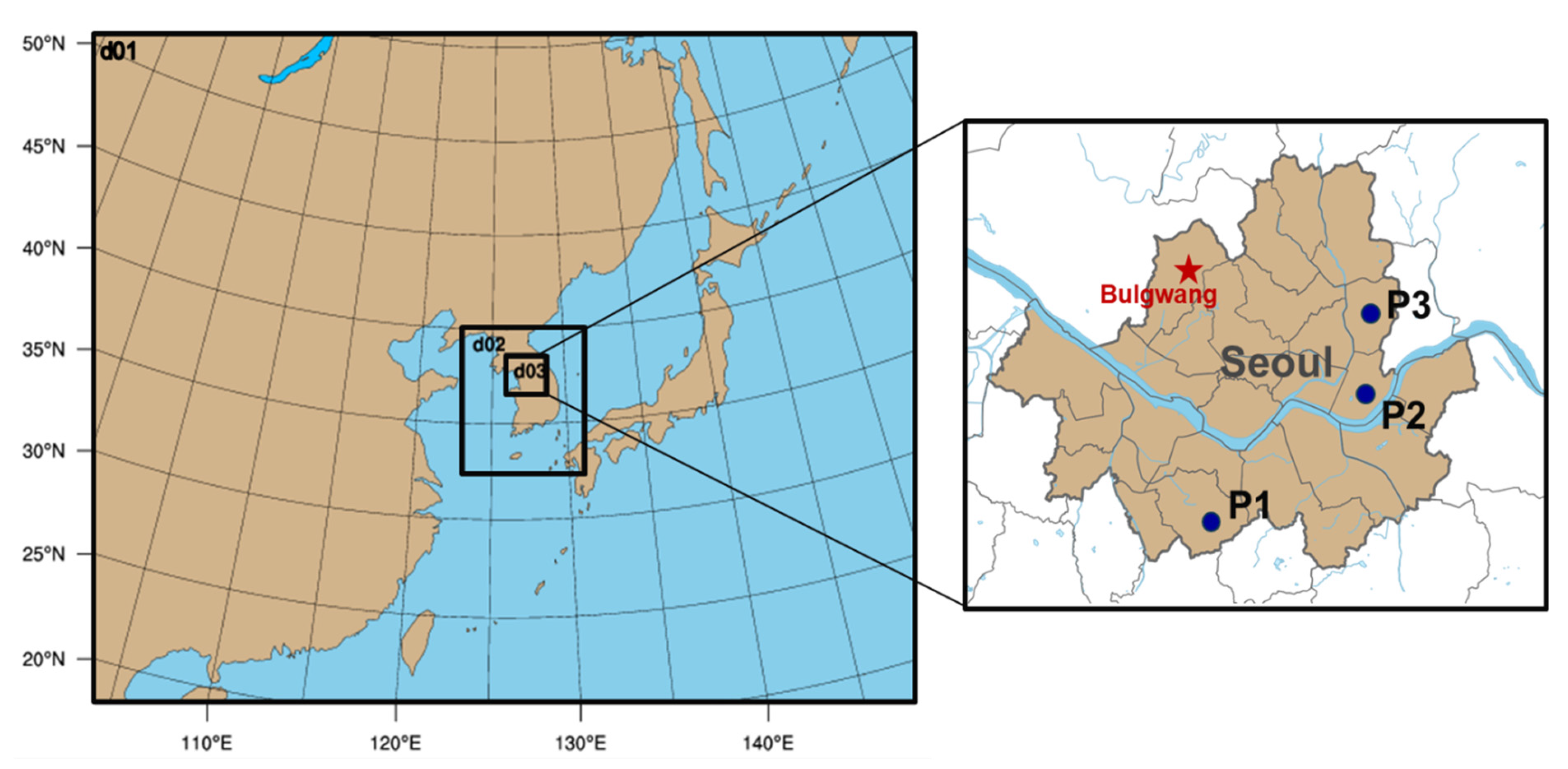
2.2. PBLH and Ground PM2.5 Measurements during the KORUS-AQ Campaign

KORUS-AQ and its pre-campaign MAPS-2015 collected comprehensive, detailed measurements of pollutants (e.g., trace gases and aerosol particles) using aircraft, ground sites, and ships with extensive spatial and vertical coverage from May 1 through June 12, 2016. During the campaign, aircraft measurements were made for the mass concentrations of PM2.5 and its chemical components; the details of aircraft measurements and ground observations have been described in numerous previous publications [29,30,31,32,33,34,35]. Because no aircraft measurements were made at night, remote ground measurements of PBLH and ground measurements of PM2.5 species were used in this study. PBLH data obtained at three sites (P1–P3) were retrieved from two remote sensing instruments: elastic aerosol lidar (AL) and wind Doppler lidar (WDL). The AL sites were located at Gwanak (P1; operated at Seoul National University) and Jungnang (P3; operated at the Weather Information Service Engine center); the WDL site was located at Gwangjin (P2; operated at the Seoul Institute of Health and Environment). PBLHs were routinely measured at time intervals of 15 min (at P1 and P2) and 1 h (at P3).
PBLHs and aerosol vertical distributions were retrieved from AL measurements using a wavelet algorithm that inferred aerosol characteristics from measured backscattering and polarization extinctions. In wavelet method, PBLH was determined as the height of sharp decrease in range-corrected backscattered intensity (β) from its vertical profile, and the Haar function was used to define sharp increases or decreases in the signal [36,37]. In this method, the PBLHs were defined as the lowest local maximum peak in the wavelet covariance profile where sharp decreases exist in the β that was identified by local maximum peaks of the wavelet covariance profile. Other aerosol characteristics (e.g., aerosol type classification, aerosol dissipation coefficient, aerosol mass concentration, and cloud base height) were also estimated from AL, but they were not retrieved when clouds were present within 2 km.
WDLs estimate PBLH in more direct approach since they directly measure the vertical wind velocity instead of vertical mixing [38,39]. WDL is primarily used to estimate wind speed profiles; it detects the wavelengths of signals backscattered from moving aerosols through the Doppler effect. WDL can also be used to measure the PBLH because it traces Doppler shifts caused by wind-derived aerosol movement and detects the outgoing aerosol signal, allowing the retrieval of wind speed [40]. We used WDL data to distinguish the nPBLH from the residual layer by applying the vertical wind profile. Prior to the use of WDL measurements, we screened wind measurements based on the signal-to-noise ratio. In this framework, PBLH can be estimated using a threshold value for vertical velocity standard deviation, σw, which was calculated based on the method of Schween et al. (2014) [41]. PBLH was then defined using a threshold value of 0.2 m/s [39] as the first height where σw drops below the threshold value. Detailed descriptions of algorithms of PBLH from AL and WDL, including data filtering criteria and data assurance, were provided by Park et al. (2021) [42] and Park et al. (2022) [43].
Ground PM2.5 measurements were conducted at Bulgwang (126.98° E, 37.61° N, 67 m a.s.l.) (Figure 1), which is close to the Jungnang site (P3). The Bulgwang site, operated by the Korean National Institute of Environmental Research, is a comprehensive measurement site for the concentrations of PM2.5 and its chemical components (e.g., sulfate, NO3, ammonium salt, organic aerosols, and gaseous precursors). For detailed analysis of PBLH–PM2.5 interactions, we used PM2.5 concentrations that had been measured at 1-h intervals with a β-ray attenuation mass monitor (BAM-1020; Met One, Grants Pass, OR, USA).

2.3. PBL Parameterizations and Sensitivity Experiment Setup

To characterize PBLH–PM2.5 interactions, we simulated PBLH and PM2.5 concentrations using the WRF-Chem model. We selected three typical PBL parameterizations: YSU, MYJ, and ACM2. The MYJ scheme is a local scheme with 1.5th-order turbulence closure; it determines the eddy diffusivity coefficient through the prognostic turbulence kinetic energy equation. The entrainment process at the top of the PBL is expressed as a function of the counter-gradient flux term characterized by large-scale eddies. Generally, MYJ shows reasonable simulation performance in a stable or weakly unstable atmosphere, as characterized by the properties of smaller eddies, but it often underestimates the PBLH in the presence of strong upward flow derived from convective turbulence activity. In contrast, YSU is a non-local scheme [44] that improves the Medium Range Forecast (MRF) scheme by enabling simulation of the shallow surface layer, where MRF cannot be applied. In the presence of strong convection in an unstable atmosphere, non-local processes are appropriate for determination of the PBLH; however, local static stability can be used to estimate the PBLH in stable conditions solely via diagnosis of the local lapse rate. The ACM2 scheme is a hybrid approach for estimation of the PBLH with non-local upstream flux in an unstable atmosphere and local downmixing in a stable atmosphere. A schematic diagram of these local and non-local PBL parameterizations is shown in Figure 2.
In terms of sensitivity experiments, we used identical meteorological physics options for three PBL mechanisms in the WRF-Chem model, then performed three PBL sensitivity simulations for the KORUS-AQ campaign period (1–31 May 2016). All options with the same meteorological components of the physics schemes (e.g., both grid- and sub-grid-scale parameterizations) were set to identical values, and only the three PBL parameterizations were varied. These model configurations allowed the detection of any inconsistencies arising from PBL parameterizations alone. A 7-day period was used for spin-up, and the WRF-Chem was run for the three PBL options to evaluate model uncertainties in the simulation of PM2.5 concentrations over the SMA.

3. Results

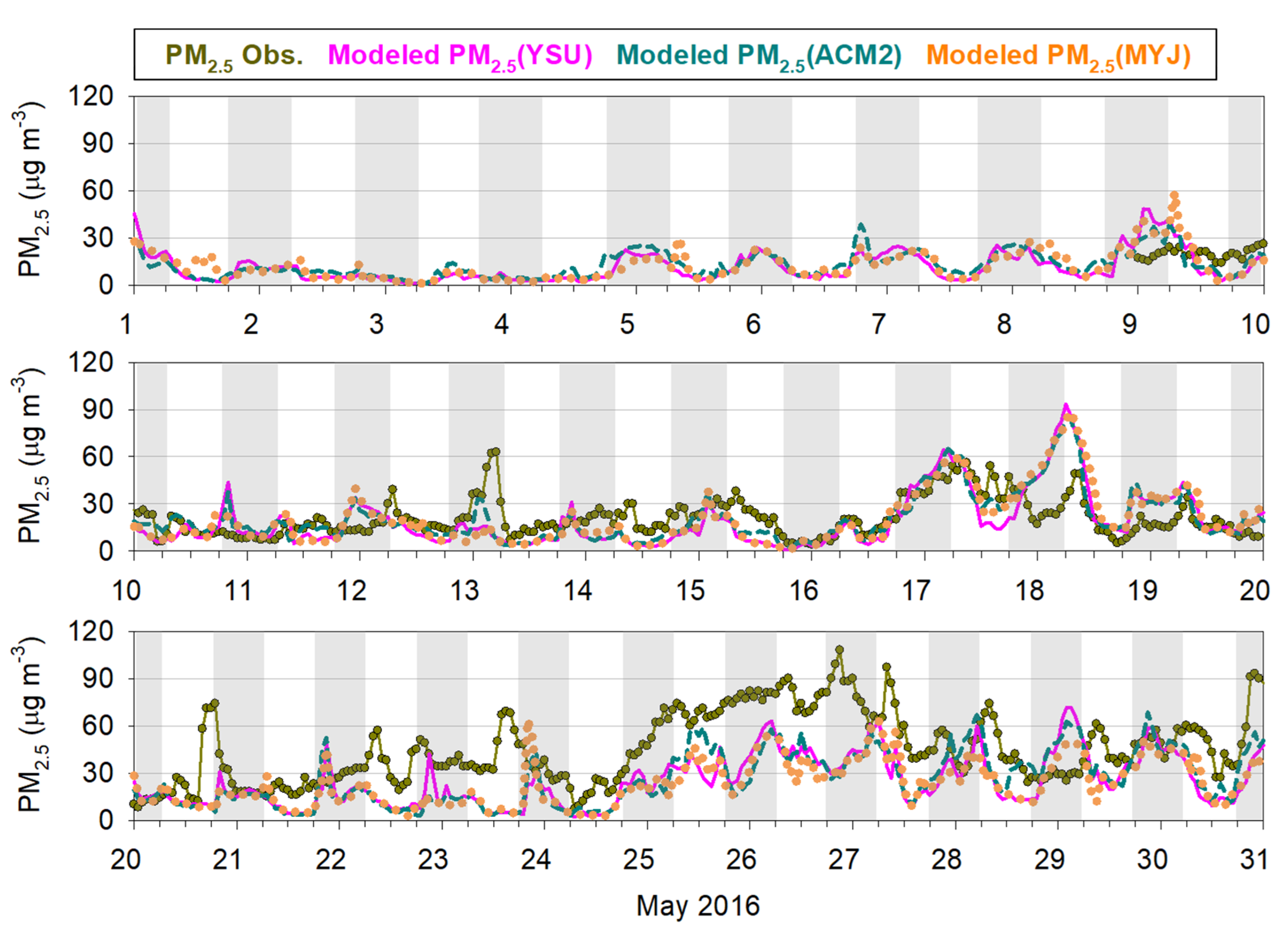
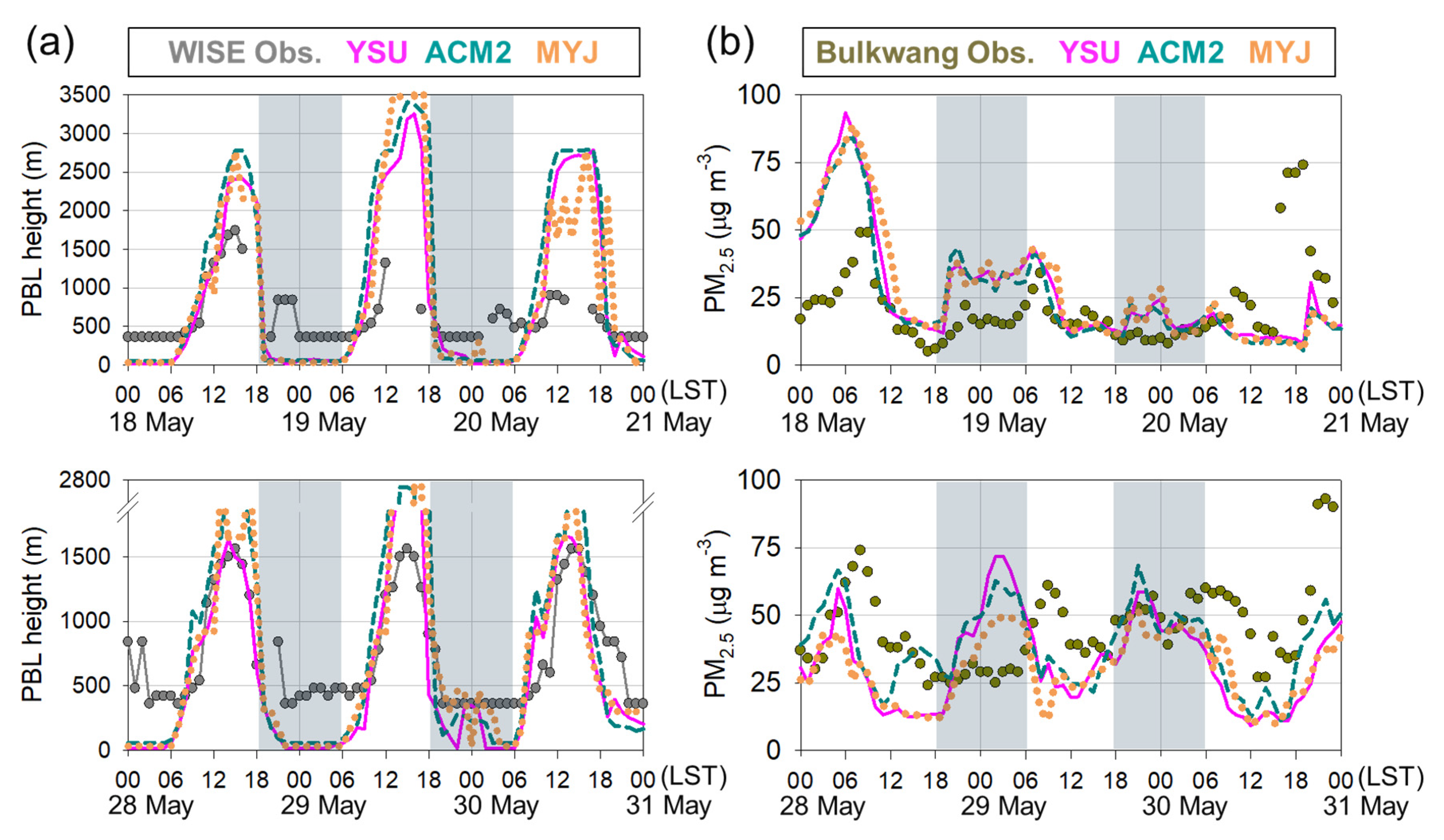
3.1. Comparison of PM2.5 Simulation Results with Observations

The PBLH and PM2.5 simulation results for the three PBL schemes at four sites (P1~P3 plus Bulgwang site) were evaluated according to the root mean square error (RMSE) (= [   ( M i O i ) 2 / N ] 1 / 2 ), normalized mean bias (NMB)(=   ( M i O i ) /   O i ), normalized mean error (NME) (=   | M i O i | /   O i ), Pearson correlation coefficient (R)(= [   ( M i M ¯ ) ( O i O ¯ ) ] / [   [ ( M i M ¯ ) 2   ( O i O ¯ ) 2 ] 1 / 2 ] ), Index of Agreement (IOA)(= 1   ( M i O i ) 2 /   ( | M i | | O i | ) 2 ), and other statistics (Table S1 and Figure 1). Here N is the number of pairs of observations/simulations, Mi is the model simulations, Oi is the observations, and M ¯ and O ¯ represent the simulated and observed means, and M’ and O’ represent Mi M ¯ and Oi O ¯ , respectively.
For PM2.5, the highest values of R (0.51) and index of agreement (0.66) were obtained using the ACM2 scheme; the lowest IOA and R values were obtained using the MYJ scheme. The three schemes simulated PM2.5 with fair IOA (0.61~0.66), but in general showed an underestimation with NMB values within −35~−30%. The root mean square error, NMB, and NME results showed similar patterns, with no significant differences among the three schemes (Table S1). Other criteria suggested by Emery et al. (2017) [46] and Choi et al. (2019) [47] are listed in Table S1 and shown Figure S1.
The observed and simulated hourly variations in PM2.5 mass concentration at the Bulgwang site during 1–31 May 2016, are shown in Figure 3. All three schemes captured the overall diurnal and weekly variations in surface PM2.5, with lower concentrations during 22–28 May. Simulation results were higher during 9–18 May (Figure 3); however, no detectable biases were observed among the three PBL schemes during this period. Overall, simulated PM2.5 mass concentrations showed temporal variations similar to the variations observed among the three schemes. We also assessed chemical components such as SO42–, NO3, NH4+, and organic carbon, with similar results among the three experiments (not shown here) and no particular biases.
Notably, the three experiments often showed significant nighttime PM2.5 concentration peaks (i.e., 18–19 May and 21–23 May). We speculate that the simulated PM2.5 concentrations were significantly overestimated, reflecting a shallow nPBLH of several tens of meters; moreover, significantly lower vertical mixing may be the result of shallow simulated nPBLH, which yielded peaks of nocturnal PM2.5 concentration peaks that were ~50 ug/m3 higher than observations (i.e., 18 May and 29 May). This result was clearly caused by extreme lower vertical mixing activity in the stable near-surface atmosphere. Further detailed analyses of the causes of nPBLH underestimation are thus needed to identify nocturnal turbulence intensities.

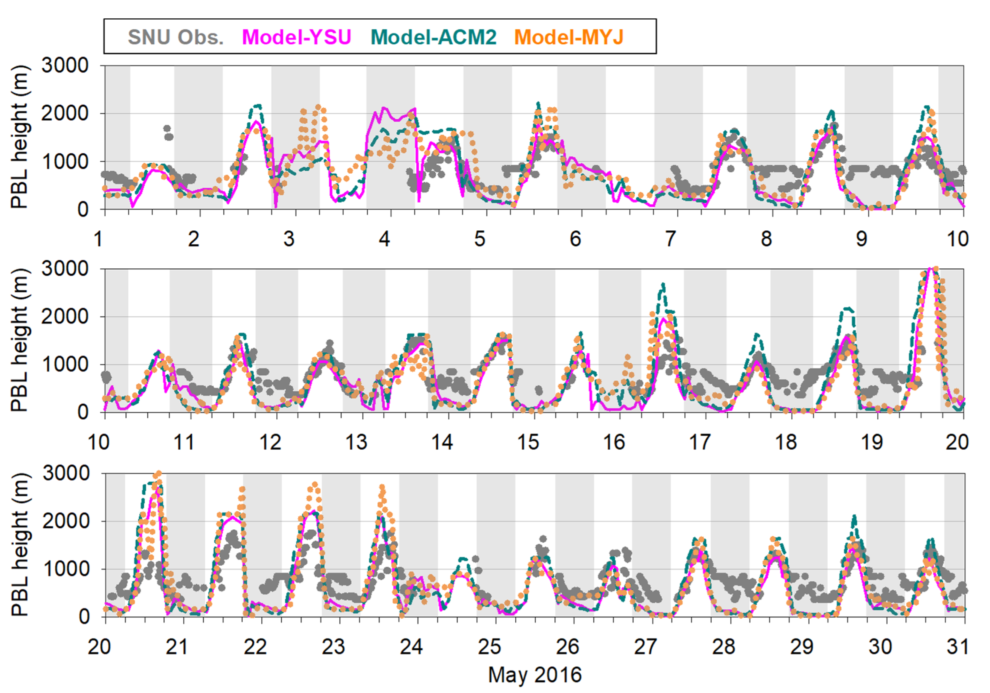
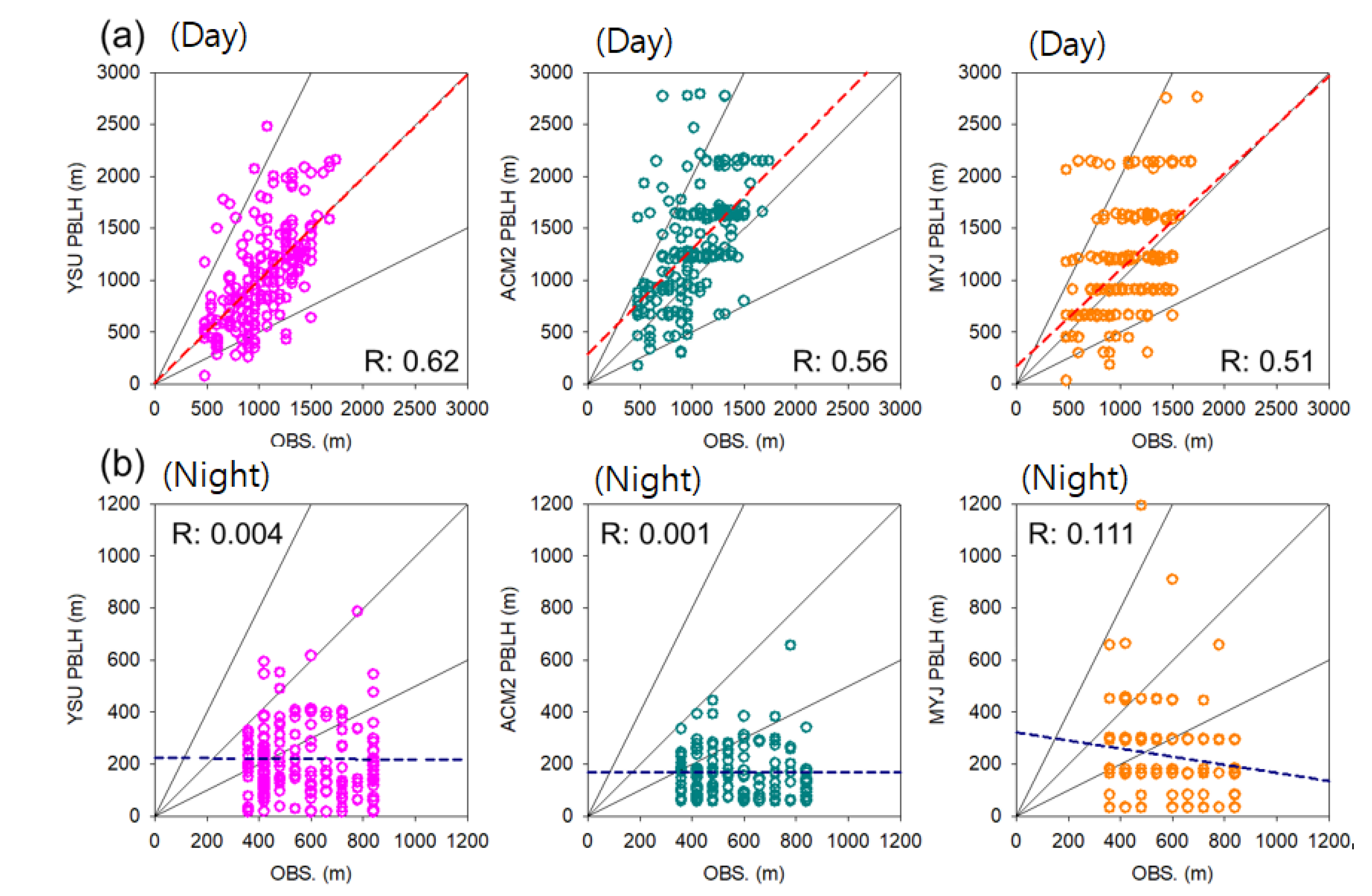
3.2. Comparison of PBLH Simulated Results with Observations

We also compared PBLH observations among the three measurement sites (P1–P3) and confirmed similar trends, with no significant differences except for a few nocturnal periods (lower at P3 on 19 May and 21–22 May) (Figure S2). The causes of these anomalies were previously discussed by Park et al. [43]; in this study, we presumed that these biases would not change the results of current study.
The time series of PBLH observed at P1 during the study period is compared with the time series of the three simulations in Figure 4. The models generally performed well in terms of simulating diurnal variations, and the results of the three sensitivity experiments were in good agreement, such that WRF-Chem overestimated the PBLH only on 21–23 May; PBLH values obtained from AL sometimes reached 1.8–2 km.
To more fully characterize the nPBLH uncertainties, we examined the large discrepancies in terms of nPBLH–PM2.5 interactions for 18–21 May and 28–31 May (Figure 5). The results showed that most daytime simulations with high discrepancies were underestimations, such as the simulations on 20 May (12:00–18:00 LST), 28 May (6:00–12:00 LST), and 29 May (6:00–18:00 LST), although PM2.5 simulations were less sensitive to PBLH overestimations during the daytime. In contrast, nighttime simulations showed the opposite trend. WRF-Chem simulated significantly lower nPBLHs, reaching 10 m in some periods: 18 May (0:00–6:00 LST), 18 May (18:00 LST) to 19 May (6:00 LST), 19 May (18:00 LST) to 20 May (6:00 LST), and 28 May (18:00 LST) to 29 May (6:00 LST). Accordingly, strong correlations were observed between nPBLH underestimation and nighttime PM2.5 overestimation. Compared with daytime PM2.5, nighttime PM2.5 was more strongly sensitive to the nPBLH (i.e., 0:00–3:00 LST on 19 May and 29 May). The shallow nPBLH caused all three simulated PM2.5 concentrations to be higher, such that they were more than twofold greater than observed values. This inverse correlation between nPBLH and PM2.5 appears to be a prerequisite factor for acceptable urban PM2.5 predictions over the SMA.

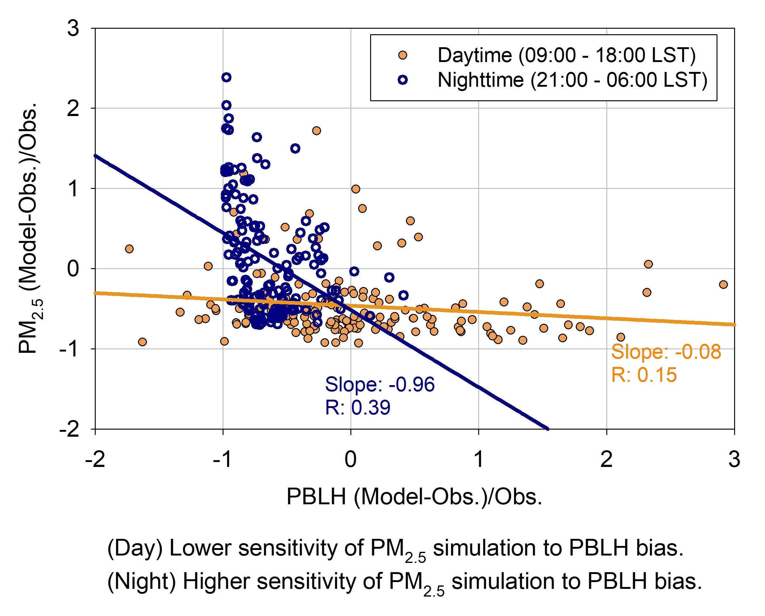
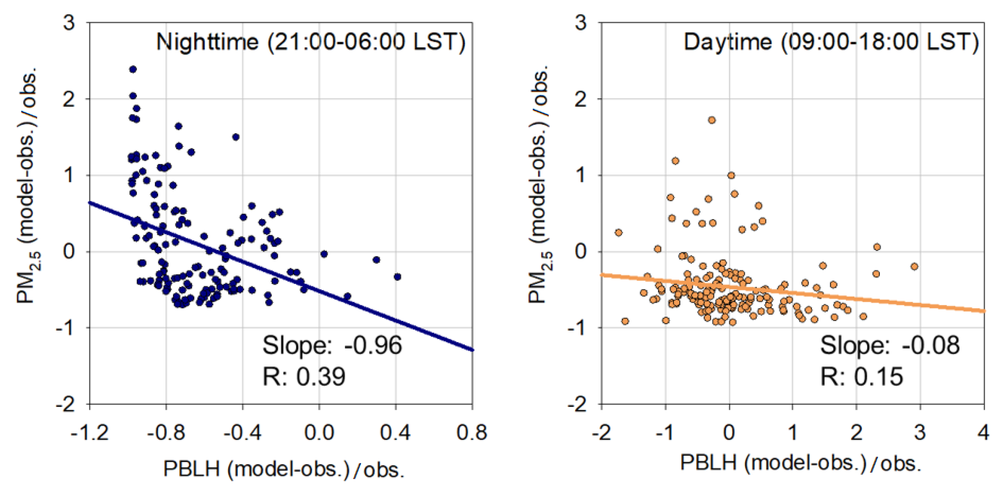
3.3. Uncertainties in Nocturnal PBLH Simulations

We sought to further characterize the uncertainty in nPBLH–PM2.5 interactions by separately comparing daytime (9:00–18:00 LST) and nighttime (21:00–06:00 LST) observations and simulations. Scatter diagrams of the results are shown in Figure 6. As expected, daytime simulations showed comparatively better agreement with observations, relative to nighttime simulations (Figure 6); correlation coefficients (R) were 0.51–0.61. Among the three experiments, the YSU scheme showed better performance for daytime simulations (R = 0.62), compared with ACM2 (R = 0.56) or MYJ (R = 0.51). However, at night, poor correlations were observed between observations and simulations (R = ~0.12), suggesting considerable model uncertainties in our nPBLH simulations. The observed nPBLHs were approximately 598 ± 124 m and the simulated values were considerably lower (213 ± 188 m [YSU], 193 ± 155 m [MYJ], and 245 ± 215 m [ACM2]), indicating underestimation by a factor of ~3. The ACM2 scheme showed better nighttime performance in terms of simulating nPBLH (R = 0.11), compared with YSU (R = 0.004) or MYJ (R = 0.001). In previous studies, non-local PBL schemes outperformed local schemes for daytime PBLH, particularly when large eddies and buoyancies were closely associated; local schemes generally outperformed non-local schemes for nighttime nPBLH, particularly when small eddies and molecular diffusion processes were better characterized on the basis of wind shear-generated mechanical turbulences in the near-surface atmosphere [48]. Our results were also consistent with previous findings regarding daytime PBLH; however, the models performed poorly in nPBLH simulations using both local and non-local schemes (R = ~0.01), with negligible differences among the three PBL schemes.
To elucidate vertical characteristics and nPBLH–PM2.5 uncertainties, we calculated normalized means differences using the formula [NMD = (S − O)/O], where S and O indicate simulations and observations, respectively. Scatter diagrams of NMD for PBLH–PM2.5 interactions during the day and night are shown in Figure 7. During the daytime the NMD of PBLH ranges from −2 to 4 while the NMD of PM2.5 approached zero (Figure 6), indicating reasonable WRF-Chem performance for daytime PM2.5. The daytime sensitivity of NMDs of PM2.5 also showed no significant tendencies according to changes in NMDs of PBLH, with lower R (−0.15) and slope (−0.08) values, indicating again low sensitivity of PM2.5 to PBLH during the daytime. However, relatively smaller NMD of nPBLH ranges from −1.2 to 0.8 during the nighttime (Figure 7) due partly to the lower nPBLH than daytime PBLH, and interactions between nPBLH and nighttime PM2.5 were stronger, with higher R (−0.39) and slope (−0.96) values between NMDs of PBLH–PM2.5. This indicates that the simulated PM2.5 is more sensitive to changes in PBLH during the nighttime. Thus, we conclude that PM2.5 responses to changes in nPBLH were greater, such that nPBLH underestimation could create bias in the peak concentrations of PM2.5, as seen on May 19, 20, 29, and 30 (Figure 5). Additional detailed investigations of the relevant characteristics are needed.
Recent PM modeling studies have revealed that the increasing NO3 fraction in PM2.5 [49] and its vertical mixing process in association with long-range transport phenomena over the Northeast Asia is becoming larger in urban areas [50], and it remains challenging to model the nocturnal formation of NO3 in association with the nighttime heterogeneous chemistry of dinitrogen pentoxide (N2O5) [12,13,14,15,51,52]. Thus, more detailed, aggregated nPBLH studies are necessary to reduce model uncertainties and improve predictions of PM concentrations in urban areas.

4. Conclusions

PBL height simulation is an important factor in predictions of PM2.5; there is a need to characterize vertical mixing processes, particularly in the stable atmosphere. In this study, we performed WRF-Chem simulations using different PBL parameterizations and explored the uncertainty associated with nPBLH–PM2.5 interactions through comparisons of the simulations with observations during the KORUS-AQ campaign (1–31 May 2016). Measurements obtained from AL and WDL, together with WRF-Chem modeling results for three different PBL parameterization schemes (YSU, MYJ, and ACM2), were used to explore these interactions and their associated uncertainties.
Our results showed that, despite lower biases in daytime PBLH simulations, both among experiments and in comparison with observations, there were large discrepancies in nPBLH simulation results for the nighttime atmosphere. WRF-Chem simulations also showed low correlation coefficient (R) values (<0.001) for all three PBL experiments at night during the KORUS-AQ campaign. Nighttime simulations consistently underestimated observation-based nPBLH by a factor of ~3 during the period because of a shallow nPBLH that created higher PM2.5 peaks.
Our normalized difference analysis of observations and simulations confirmed that the sensitivity of lower PBLHs to PM2.5 was greater at night, such that uncertainties in nPBLH easily led to failure in the prediction of nPM2.5 levels in the nighttime atmosphere. In the absence of direct evidence or observations to link shallow nPBLH and PM2.5, a thorough knowledge of nocturnal PBL dynamics from further comparisons of measurements and simulations is needed to sufficiently improve estimates of PM2.5 concentrations.
We conclude that there is a need to characterize stable atmosphere vertical mixing processes, but this characterization depends on an improvement of nPBLH uncertainties that involves additional observational data and the resolution of limitations within air quality models. Therefore, a well-designed nocturnal field experiment is necessary to elucidate the complexities of key processes that control the nPBLH. Additional model sensitivity studies should be performed under various atmospheric meteorological conditions to provide a legitimate and integrative evaluation of nPBLH schemes in urban areas.

Supplementary Materials

The following supporting information can be downloaded at: https://www.mdpi.com/article/10.3390/rs15020300/s1, Figure S1: Comparisons of WRF-Chem simulation performance against observed PBLH at Gwanak (P1), Gwangjin (P2), and Jungnang (P3) and measured PM2.5 at Seoul-Bulgwang; Figure S2: Comparison between PBLH observations at P1 (Gwanak), P2 (Gwangjin) and P3 (Jungnang); Table S1: ummary statistics for comparison between WRF-Chem simulations and observed PBLH at Gwanak (P1), Gwangjin (P2), and Jungnang (P3) and measured PM2.5 at Seoul-Bulgwang.

Author Contributions

Conceptualization and writing—original draft preparation, H.-J.L.; Methodology, writing—review and editing, C.-H.K.; Measurements and formal analysis, M.-S.P.; Model simulation and analysis, H.-Y.J. and J.-M.K.; Data curation, J.B., J.-K.K. and Y.-J.J.; Investigation, C.-H.K.; All authors have read and agreed to the published version of the manuscript.

Funding

This research was supported by the Basic Science Research Program through the National Research Foundation of Korea (NRF) funded by the Ministry of Education (2020R1I1A2075417) and funded by the Korean government (MSIT) (NRF-2022R1A2C1008132).

Data Availability Statement

All modeling and measured data including hourly planetary boundary layer heights observed by both elastic aerosol lidar and wind Doppler lidar, and surface PM2.5 measurements related to this paper are available from the corresponding author on reasonable request.

Acknowledgments

We would like to express our gratitude to Sang-Woo Kim at Seoul National University for providing wind Doppler lidar measurements. The authors are also grateful to the anonymous reviewers for their comments.

Conflicts of Interest

The authors declare no conflict of interest.

References

  1. Marcazzan, G.M.; Vaccaro, S.; Valli, G.; Vecchi, R. Characterisation of PM10 and PM2.5 particulate matter in the ambient air of Milan (Italy). Atmos. Environ. 2001, 35, 4639–4650. [Google Scholar] [CrossRef]
  2. Fuzzi, S.; Baltensperger, U.; Carslaw, K.; Decesari, S.; Denier van der Gon, H.; Facchini, M.C.; Fowler, D.; Koren, I.; Langford, B.; Lohmann, U.; et al. Particulate matter, air quality and climate: Lessons learned and future needs. Atmos. Chem. Phys. 2015, 15, 8217–8299. [Google Scholar]
  3. Chiashi, A.; Lee, S.; Pollitt, H.; Chewpreecha, U.; Vercoulen, P.; He, Y.; Xu, B. Transboundary PM Air Pollution and Its Impact on Health in East Asia. In Energy, Environmental and Economic Sustainability in East Asia: Policies and Institutional Reforms; Lee, S., Pollitt, H., Fujikawa, K., Eds.; Routledge: London, UK, 2019. [Google Scholar]
  4. Shapiro, M. Transboundary Air Pollution in Northeast Asia: The Political Economy of Yellow Dust, Particulate Matter, and PM2.5. In KEI Academic Paper Series; Korea Economic Institute of America: Washington, DC, USA, 2016. [Google Scholar]
  5. McConnell, R.; Berhane, K.; Gilliland, F.; Molitor, J.; Thomas, D.; Lurmann, F. Prospective study of air pollution and bronchitic symptoms in children with asthma. Am. J. Respir. Crit. Care Med. 2003, 168, 790–797. [Google Scholar] [CrossRef] [PubMed] [Green Version]
  6. He, M.; Ichinose, T.; Yoshida, Y.; Arashidani, K.; Yoshida, S.; Takano, H.; Sun, G.; Shibamoto, T. Urban PM2.5 exacerbates allergic inflammation in the murine lung via a TLR2/TLR4/MyD88-signaling pathway. Sci. Rep. 2017, 7, 11027. [Google Scholar] [CrossRef] [Green Version]
  7. Turner, M.C.; Cohen, A.; Burnett, R.T.; Jerrett, M.; Diver, W.R.; Gapstur, S.M.; Krewski, D.; Samet, J.M.; Pope, C.A. Interactions between cigarette smoking and ambient PM2.5 for cardiovascular mortality. Environ. Res. 2017, 154, 304–310. [Google Scholar] [CrossRef]
  8. Lang, J.; Zhang, Y.; Zhou, Y.; Cheng, S.; Chen, D.; Guo, X.; Chen, S.; Li, X.; Xing, X.; Wang, H. Trends of PM2.5 and chemical composition in Beijing, 2000~2015. Aerosol Air Qual. Res. 2017, 17, 412–425. [Google Scholar] [CrossRef] [Green Version]
  9. Kang, Y.-H.; You, S.; Bae, M.; Kim, E.; Son, K.; Bae, C.; Kim, Y.; Kim, B.-U.; Kim, H.C.; Kim, S. The impacts of COVID-19, meteorology, and emission control policies on PM2.5 drops in Northeast Asia. Sci. Rep. 2020, 10, 22112. [Google Scholar] [CrossRef]
  10. Miao, Y.; Li, J.; Miao, S.; Che, H.; Wang, Y.; Zhang, X.; Zhu, R.; Liu, S. Interaction between Planetary Boundary Layer and PM2.5 Pollution in Megacities in China: A Review. Curr. Pollut. Rep. 2019, 5, 261–271. [Google Scholar] [CrossRef] [Green Version]
  11. Stull, R.B. An Introduction to Boundary Layer Meteorology; Springer: Dordrecht, The Netherlands, 1988. [Google Scholar]
  12. Pathak, R.K.; Wu, W.S.; Wang, T. Summertime PM2.5 ionic species in four major cities of China: Nitrate formation in an ammonia-deficient atmosphere. Atmos. Chem. Phys. 2009, 9, 1711–1722. [Google Scholar] [CrossRef] [Green Version]
  13. Brown, S.S.; Ryerson, T.B.; Wollny, A.G.; Brock, C.A.; Peltier, R.; Sullivan, A.P.; Weber, R.J.; Dube, W.P.; Trainer, M.; Meagher, J.F.; et al. Variability in nocturnal nitrogen oxide processing and its role in regional air quality. Science 2006, 311, 67–70. [Google Scholar] [CrossRef]
  14. Jo, H.-Y.; Lee, H.-J.; Jo, Y.-J.; Lee, J.-J.; Ban, S.; Lee, J.-J.; Chang, L.-S.; Heo, G.; Kim, C.-H. Nocturnal fine particulate nitrate formation by N2O5 heterogeneous chemistry in Seoul Metropolitan Area, Korea. Atmos. Res. 2019, 225, 58–69. [Google Scholar] [CrossRef]
  15. Jo, H.-Y.; Lee, H.-J.; Jo, Y.-J.; Heo, G.; Lee, M.; Kim, J.-A.; Park, M.-S.; Lee, T.; Kim, S.-W.; Lee, Y.-H.; et al. A case study of heavy PM2.5 secondary formation by N2O5 nocturnal chemistry in Seoul, Korea in January 2018: Model performance and error analysis. Atmos. Res. 2022, 266, 105951. [Google Scholar] [CrossRef]
  16. Steeneveld, G.J.; Mauritsen, T.; DeBruijn, E.I.F.; De Arellano, J.V.G.; Svensson, G.; Holtslag, A.A.M. Evaluation of limited-area models for the representation of the diurnal cycle and contrasting nights in CASES-99. J. Appl. Meteorol. Climatol. 2008, 47, 869–887. [Google Scholar] [CrossRef]
  17. Storm, B.; Dudhia, J.; Basu, S.; Swift, A.; Giammanco, I. Evaluation of the Weather Research and Forecasting model on forecasting low-level jets: Implications for wind energy. Wind Energy 2009, 12, 81–90. [Google Scholar] [CrossRef]
  18. Hu, X.-M.; Doughty, D.C.; Sanchez, K.J.; Joseph, E.; Fuentes, J.D. Ozone variability in the atmospheric boundary layer in Maryland and its implications for vertical transport model. Atmos. Environ. 2012, 46, 354–364. [Google Scholar] [CrossRef]
  19. García Diez, M.; Fernández, J.; Fitaand, L.; Yague, C. Seasonal dependence of WRF model biases and sensitivity to PBL schemes over Europe. Q. J. R. Meteorol. Soc. 2013, 139, 501–514. [Google Scholar] [CrossRef] [Green Version]
  20. Boadh, R.; Satyanarayana, A.N.V.; Rama Krishna, T.V.B.P.S.; Madala, S. Sensitivity of PBL schemes of the WRF-ARW model in simulating the boundary layer flow parameters for their application to air pollution dispersion modeling over a tropical station. Atmósfera 2016, 29, 61–81. [Google Scholar] [CrossRef] [Green Version]
  21. Li, Y.; Du, A.; Lei, L.; Sun, J.; Li, Z.; Zhang, Z.; Wang, Q.; Tang, G.; Song, S.; Wang, Z.; et al. Vertically Resolved Aerosol Chemistry in the Low Boundary Layer of Beijing in Summer. Environ. Sci. Technol. 2022, 56, 9312–9324. [Google Scholar] [CrossRef]
  22. Crawford, J.H.; Ahn, J.-Y.; Al-Saadi, J.; Chang, L.; Emmons, L.K.; Kim, J.; Lee, G.; Park, J.-H.; Park, R.J.; Woo, J.H.; et al. The Korea–United States Air Quality (KORUS-AQ) field study. Elem. Sci. Anthr. 2021, 9, 00163. [Google Scholar] [CrossRef]
  23. Kim, C.-H.; Lee, H.-J.; Kang, J.-E.; Jo, H.-Y.; Park, S.-Y.; Jo, Y.-J.; Lee, J.-J.; Yang, G.-H.; Park, T.; Lee, T. Meteorological Overview and Signatures of Long-range Transport Processes during the MAPS-Seoul 2015 Campaign. Aerosol Air Qual. Res. 2018, 18, 2173–2184. [Google Scholar] [CrossRef] [Green Version]
  24. Park, R.J.; Oak, Y.J.; Emmons, L.K.; Kim, C.-H.; Pfister, G.G.; Carmichael, G.R.; Saide, P.E.; Cho, S.-Y.; Kim, S.; Woo, J.-H.; et al. Multi-model intercomparisons of air quality simulations for the KORUS-AQ campaign. Elem. Sci. Anthr. 2021, 9, 00139. [Google Scholar] [CrossRef]
  25. Kurokawa, J.; Ohara, T.; Morikawa, T.; Hanayama, S.; Janssens-Maenhout, G.; Fukui, T.; Kawashima, K.; Akimoto, H. Emissions of air pollutants and greenhouse gases over Asian regions during 2000–2008: Regional Emission inventory in ASia (REAS) version 2. Atmos. Chem. Phys. 2013, 13, 11019–11058. [Google Scholar] [CrossRef] [Green Version]
  26. Lee, D.-G.; Lee, Y.-M.; Jang, K.-W.; Yoo, C.; Kang, K.-H.; Lee, J.-H.; Jung, S.-W.; Park, J.-M.; Lee, S.-B.; Han, J.-S.; et al. Korean National Emissions Inventory System and 2007 Air Pollutant Emissions. Asian J. Atmos. Environ. 2011, 5, 278–291. [Google Scholar] [CrossRef] [Green Version]
  27. Woo, J.-H.; Choi, K.-C.; Kim, H.K.; Baek, B.H.; Jang, M.; Eum, J.-H.; Song, C.H.; Ma, Y.-L.; Sunwoo, Y.; Chang, L.-S.; et al. Development of an anthropogenic emissions processing system for Asia using SMOKE. Atmos. Environ. 2012, 58, 5–13. [Google Scholar] [CrossRef]
  28. Yang, G.-H.; Jo, Y.-J.; Lee, H.-J.; Song, C.-K.; Kim, C.-H. Numerical Sensitivity Tests of Volatile Organic Compounds Emission to PM2.5 Formation during Heat Wave Period in 2018 in Two Southeast Korean Cities. Atmosphere 2020, 11, 331. [Google Scholar] [CrossRef] [Green Version]
  29. Lee, H.-J.; Jo, H.-Y.; Song, C.-K.; Jo, Y.-J.; Park, S.-Y.; Kim, C.-H. Sensitivity of Simulated PM2.5 Concentrations over Northeast Asia to Different Secondary Organic Aerosol Modules during the KORUS-AQ Campaign. Atmosphere 2020, 11, 1004. [Google Scholar] [CrossRef]
  30. Lee, H.-J.; Jo, H.-Y.; Park, S.-Y.; Jo, Y.-J.; Jeon, W.; Ahn, J.-Y.; Kim, C.-H. A Case Study of the Transport/Transformation of Air Pollutants Over the Yellow Sea During the MAPS 2015 Campaign. J. Geophys. Res. Atmos. 2019, 124, 6532–6553. [Google Scholar] [CrossRef]
  31. Jayne, J.T.; Leard, D.C.; Zhang, X.; Davidovits, P.; Smith, K.A.; Kolb, C.E.; Worsnop, D.R. Development of an Aerosol Mass Spectrometer for Size and Composition Analysis of Submicron Particles. Aerosol Sci. Technol. 2000, 33, 49–70. [Google Scholar] [CrossRef] [Green Version]
  32. Jimenez, J.L.; Jayne, J.T.; Shi, Q.; Kolb, C.E.; Worsnop, D.R.; Yourshaw, I.; Seinfeld, J.H.; Flagan, R.C.; Zhang, X.; Smith, K.A.; et al. Ambient aerosol sampling using the Aerodyne Aerosol Mass Spectrometer. J. Geophys. Res. Atmos. 2003, 108, 8425. [Google Scholar] [CrossRef] [Green Version]
  33. Drewnick, F.; Hings, S.S.; DeCarlo, P.; Jayne, J.T.; Gonin, M.; Fuhrer, K.; Weimer, S.; Jimenez, J.L.; Demerjian, K.L.; Borrmann, S.; et al. A New Time-of-Flight Aerosol Mass Spectrometer (TOF-AMS)—Instrument Description and First Field Deployment. Aerosol Sci. Technol. 2005, 39, 637–658. [Google Scholar] [CrossRef]
  34. DeCarlo, P.F.; Kimmel, J.R.; Trimborn, A.; Northway, M.J.; Jayne, J.T.; Aiken, A.C.; Gonin, M.; Fuhrer, K.; Horvath, T.; Docherty, K.S.; et al. Field-Deployable, High-Resolution, Time-of-Flight Aerosol Mass Spectrometer. Anal. Chem. 2006, 78, 8281–8289. [Google Scholar] [CrossRef]
  35. Canagaratna, M.R.; Jayne, J.T.; Jimenez, J.L.; Allan, J.D.; Alfarra, M.R.; Zhang, Q.; Onasch, T.B.; Drewnick, F.; Coe, H.; Middlebrook, A.; et al. Chemical and microphysical characterization of ambient aerosols with the aerodyne aerosol mass spectrometer. Mass Spectrom. Rev. 2007, 26, 185–222. [Google Scholar] [CrossRef] [PubMed]
  36. Brooks, I.M. Finding Boundary Layer Top: Application of a Wavelet Covariance Transform to Lidar Backscatter Profiles. J. Atmos. Ocean. Technol. 2003, 20, 1092–1105. [Google Scholar] [CrossRef]
  37. Caicedo, V.; Rappenglück, B.; Lefer, B.; Morris, G.; Toledo, D.; Delgado, R. Comparison of aerosol lidar retrieval methods for boundary layer height detection using ceilometer aerosol backscatter data. Atmos. Meas. Tech. 2017, 10, 1609. [Google Scholar] [CrossRef] [Green Version]
  38. Park, S.; Kim, S.-W.; Park, M.-S.; Song, C.-K. Measurements of planetary boundary layer winds with scanning Doppler lidar. Remote Sens. 2018, 10, 1261. [Google Scholar] [CrossRef] [Green Version]
  39. Tucker, S.C.; Brewer, W.A.; Banta, R.M.; Senff, C.J.; Sandberg, S.P.; Law, D.C.; Weickmann, A.M.; Hardesty, R.M. Doppler lidar estimation of mixing height using turbulence, shear, and aerosol profiles. J. Atmos. Oceanic Tech. 2009, 26, 673–688. [Google Scholar] [CrossRef]
  40. Werner, C. Doppler Wind Lidar. In Lidar: Range-Resolved Optical Remote Sensing of the Atmosphere; Weitkamp, C., Ed.; Springer: New York, NY, USA, 2005; pp. 325–354. ISBN 978-0-387-25101-1. [Google Scholar]
  41. Schween, J.H.; Hirsikko, A.; Lohnert, U.; Crewell, S. Mixing-layer height retrieval with ceilometer and Doppler lidar: From case studies to long-term assessment. Atmos. Meas. Tech. 2014, 7, 3685–3704. [Google Scholar]
  42. Park, D.-H.; Kim, S.-W.; Kim, M.-H.; Yeo, H.; Park, S.S.; Nishizawa, T.; Shimizu, A.; Kim, C.-H. Impacts of local versus long-range transported aerosols on PM10 concentrations in Seoul, Korea: An estimate based on 11-year PM10 and lidar observations. Sci. Total Environ. 2021, 750, 141739. [Google Scholar] [CrossRef]
  43. Park, S.; Kim, M.-H.; Yeo, H.; Shim, K.; Lee, H.-J.; Kim, C.-H.; Song, C.-K.; Park, M.-S.; Shimizu, A.; Nishizawa, T.; et al. Determination of mixing layer height from co-located lidar, ceilometer and wind Doppler lidar measurements: Intercomparison and implications for PM2.5 simulations. Atmos. Pollut. Res. 2022, 13, 101310. [Google Scholar] [CrossRef]
  44. Hong, S.-Y.; Kim, J.-H.; Lim, J.-O.; Dudhia, J. The WRF single–moment 6–class microphysics scheme (WSM6). J. Korean Meteor. Soc. 2006, 42, 129–151. [Google Scholar]
  45. Ahasan, M.N.; Chowdhury, M.A.M.; Quadir, D.A. Sensitivity Test of Parameterization Schemes of MM5 Model for Prediction of the High Impact Rainfall Events over Bangladesh. J. Mech. Eng. 2014, 44, 33–42. [Google Scholar] [CrossRef] [Green Version]
  46. Emery, C.; Liu, Z.; Russell, A.G.; Odman, M.T.; Yarwood, G.; Kumar, N. Recommendations on statistics and benchmarks to assess photochemical model performance. J. Air Waste Manag. Assoc. 2017, 67, 582–598. [Google Scholar] [CrossRef] [PubMed] [Green Version]
  47. Choi, M.-W.; Lee, J.-H.; Woo, J.-W.; Kim, C.-H.; Lee, S.-H. Comparison of PM2.5 Chemical Components over East Asia Simulated by the WRF-Chem and WRF/CMAQ Models: On the Models’ Prediction Inconsistency. Atmosphere 2019, 10, 618. [Google Scholar] [CrossRef]
  48. Jung, S.Y.; Kim, C.H. Bias Analysis of WRF-CMAQ Simulated PM2.5 Concentration Caused by Different PBL Parameterizations: Application to the Haze period of March in 2019 over the Seoul Metropolitan Area. J. Korean Soc. Atmos. Environ. 2021, 37, 835–852, (In Korean with English Abstract). [Google Scholar] [CrossRef]
  49. Jo, Y.-J.; Lee, H.-J.; Jo, H.-Y.; Woo, J.-H.; Kim, Y.; Lee, T.; Heo, G.; Park, S.-M.; Jung, D.; Park, J. Changes in inorganic aerosol compositions over the Yellow Sea area from impact of Chinese emissions mitigation. Atmos. Res. 2020, 240, 104948. [Google Scholar] [CrossRef]
  50. Lee, H.J.; Jo, H.Y.; Kim, S.W.; Park, M.S.; Kim, C.H. Impacts of Atmospheric Vertical Structures on Transboundary Aerosol Transport from China to South Korea. Sci. Rep. 2019, 9, 13040. [Google Scholar] [CrossRef] [PubMed] [Green Version]
  51. Brown, S.G.; Roberts, P.T.; McCarthy, M.C.; Lurmann, F.W. Wintertime vertical variations in particulate matter (PM) and precursor concentrations in the San Joaquin valley during the California regional coarse PM/Fine PM air quality study. J. Air Waste Manage. Assoc. 2006, 56, 1267–1277. [Google Scholar] [CrossRef] [Green Version]
  52. Prabhakar, G.; Parworth, C.L.; Zhang, X.; Kim, H.; Young, D.E.; Beyersdorf, A.J.; Ziemba, L.D.; Nowak, J.B.; Bertram, T.H.; Faloona, I.C.; et al. Observational assessment of the role of nocturnal residual-layer chemistry in determining daytime surface particulate nitrate concentrations. Atmos. Chem. Phys. 2017, 17, 14747–14770. [Google Scholar] [CrossRef]
Figure 1. Three nested domains were implemented in the Weather Research and Forecasting regional air quality and chemistry model (WRF-Chem): D01 (grid spacing, 27 km; Northeast Asia), D02 (9 km; Korean Peninsula), and D03 (3 km; South Korea). Three planetary boundary layer height (PBLH) observation sites are shown: Gwanak (P1), Gwangjin (P2), and Jungnang (P3). An air quality measurement site (Bulgwang) is also shown.
Remotesensing 15 00300 g001
Figure 2. Schematic of local and non-local mixing processes in the PBL (modified from Ahasan et al., 2014 [45]).
Remotesensing 15 00300 g002
Figure 3. Measured and simulated particulate matter (PM2.5) concentrations at the Bulgwang site during the Korea–United States Air Quality Study (KORUS-AQ) campaign (May 2016). Data are observations (green) and WRF-Chem simulations from three different PBL parameterizations: Yonsei University (YSU, pink), Asymmetrical Convective Model v2 (ACM2, blue), and Mellor–Yamada–Janjic (MYJ, orange). Gray shaded area indicates nighttime (21:00–6:00 LST).
Remotesensing 15 00300 g003
Figure 4. Comparison of PBLH between observations at P1 (Gwanak; gray) and simulated values obtained using the YSU (pink), ACM2 (blue), and MYJ (orange) parameterization schemes in the WRF-Chem model. Gray shaded area indicates nighttime (21:00–6:00 LST).
Remotesensing 15 00300 g004
Figure 5. Temporal variations in (a) PBLH observations at the P3 site and (b) PM2.5 observations at the Bulgwang site compared with simulations using the YSU, MYJ, and ACM2 PBL schemes for the periods 18–21 May and 28–31 May 2016. Gray shaded area indicates night.
Remotesensing 15 00300 g005
Figure 6. Scatter diagrams of simulated and observed PBLHs at P1 (Gwanak). PBL schemes included YSU (pink), ACM2 (blue), and MYJ (orange) parameterizations for (a) daytime (09:00–18:00 LST) and (b) nighttime (21:00–6:00 LST) simulations.
Remotesensing 15 00300 g006
Figure 7. Scatter diagrams of normalized means differences [NMD = (S − O)/O] between PBLH versus PM2.5 interactions for daytime (09:00–18:00 LST) (left) and nighttime (21:00–6:00 LST) (right) simulations. Here S and O indicate simulations and observations, respectively.
Remotesensing 15 00300 g007
Table 1. Summary of physical and chemical options used in Weather Research and Forecasting regional air quality and chemistry model (WRF-Chem) simulations in this study.
Physics OptionAdopted Scheme
MicrophysicsLin et al. scheme
Longwave radiationRapid radiative transfer model (RRTM)
Shortwave radiationGoddard
Surface layerMonin–Obukhov similarity
Land surfaceNoah Land Surface Model
Planetary boundary layerYonsei University scheme (YSU)/Mellor-Yamada-Janjic (MYJ)/Asymmetric Convective Model, version 2 (ACM2)
Cumulus parameterizations Grell 3-D
Chemistry optionAdopted scheme
PhotolysisMadronich photolysis (TUV)
Gas phase chemistryNOAA/ESRL Regional Atmospheric Chemistry (RACM)
AerosolsModal Approach Dynamics model for Europe/Volatility Basis Set (MADE/VBS)
Anthropogenic emissionsKORUS v2
Biogenic emissionsModel of Emissions of Gases and Aerosols from Nature (MEGAN) v2.04
Disclaimer/Publisher’s Note: The statements, opinions and data contained in all publications are solely those of the individual author(s) and contributor(s) and not of MDPI and/or the editor(s). MDPI and/or the editor(s) disclaim responsibility for any injury to people or property resulting from any ideas, methods, instructions or products referred to in the content.

