Article

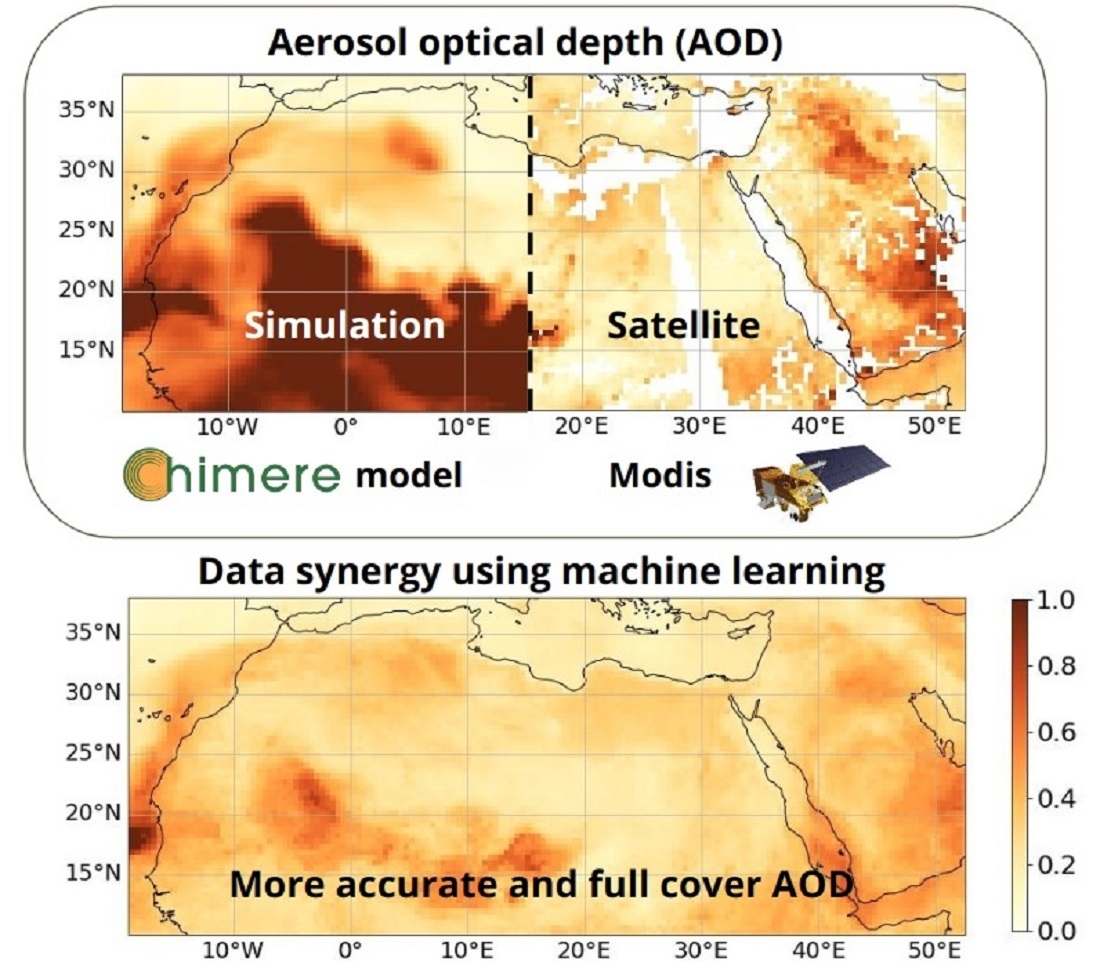
Machine Learning-Based Improvement of Aerosol Optical Depth from CHIMERE Simulations Using MODIS Satellite Observations

1
Univ. Paris Est Creteil and Université Paris Cité, CNRS, LISA, F-94010 Créteil, France
2
ARIA Technologies, F-92100 Boulogne-Billancourt, France
3
Nansen Environmental and Remote Sensing Center (NERSC), N-5007 Bergen, Norway
4
Université de Paris Cité and Univ. Paris Est Creteil, CNRS, LISA, F-75013 Paris, France
*
Author to whom correspondence should be addressed.
Remote Sens. 2023, 15(6), 1510; https://doi.org/10.3390/rs15061510
Submission received: 31 January 2023 / Revised: 1 March 2023 / Accepted: 6 March 2023 / Published: 9 March 2023

Abstract

:
We present a supervised machine learning (ML) approach to improve the accuracy of the regional horizontal distribution of the aerosol optical depth (AOD) simulated by the CHIMERE chemistry transport model over North Africa and the Arabian Peninsula using Moderate Resolution Imaging Spectroradiometer (MODIS) AOD satellite observations. Our method produces daily AOD maps with enhanced precision and full spatial domain coverage, which is particularly relevant for regions with a high aerosol abundance, such as the Sahara Desert, where there is a dramatic lack of ground-based measurements for validating chemistry transport simulations. We use satellite observations and some geophysical variables to train four popular regression models, namely multiple linear regression (MLR), random forests (RF), gradient boosting (XGB), and artificial neural networks (NN). We evaluate their performances against satellite and independent ground-based AOD observations. The results indicate that all models perform similarly, with RF exhibiting fewer spatial artifacts. While the regression slightly overcorrects extreme AODs, it remarkably reduces biases and absolute errors and significantly improves linear correlations with respect to the independent observations. We analyze a case study to illustrate the importance of the geophysical input variables and demonstrate the regional significance of some of them.

Graphical Abstract

1. Introduction

Particulate matter suspended in the air, known as aerosols, has a major impact on the environment. The scattering and absorption of radiation by aerosols (e.g., desert dust and black carbon) significantly alters the Earth’s radiative balance and consequently affects the climate system [1,2,3,4]. Aerosols are also the most important air pollutants and the greatest environmental threat to human health, causing more than 3 million premature deaths worldwide each year [5]. Therefore, it is of a great importance to estimate and predict the spatial distribution and variability of aerosols and their interaction with radiation. The latter is described by their optical properties, such as the aerosol optical depth (AOD).
Satellite measurements, such as those derived from the Moderate Resolution Imaging Spectroradiometer (MODIS) spaceborne sensor [6], play a fundamental role in observing the spatial distribution of aerosols at the global scale. These remote sensing observations are mainly derived in terms of the AOD, which describes the total column extinction that is integrated over the whole atmosphere. They therefore provide maps of the horizontal distribution of aerosol abundance. However, they are only available for cloud-free conditions and are limited by the overpass time of the (polar orbiting) satellite. On the other hand, chemistry transport models (CTMs), such as CHIMERE [7], numerically simulate the hourly 3D evolution of aerosol plumes in the atmosphere, independent of the cloudiness. The accuracy of the CTM simulations depends on the precision of the inputs, e.g., the emissions of atmospheric constituents, wind, vertical velocity fields, and on the assumed aerosol properties (e.g., microphysical and optical properties). Due to assumptions and inaccuracies in these datasets, simulations of the aerosol spatial distribution are prone to bias compared to observations [8,9]. These errors are related to uncertainties in the physical parameterizations of the model, input data, and numerical approximations [10]. Modeling errors are more pronounced in regions lacking ground-based stations to validate and constrain the simulations, which is the case for the African continent and the Middle East.
Most of the techniques used to constrain chemistry transport models use ground-based in situ measurements and, more recently, satellite data such as MODIS AOD, e.g., for the North African mineral dust emissions inversion [11,12] and for the Copernicus Atmosphere Monitoring Service (CAMS) [13]. They are mainly based on data assimilation techniques such as variational or filtering approaches [14], which are computationally expensive. On the other hand, fast and computationally efficient approaches use machine learning (ML) techniques to correct the modeling systematic biases. These methods are increasingly being used due to the progress in the development of ML hardware and technology. ML bias correction techniques are mainly used for chemistry transport model simulations of trace gases, e.g., [15], or used in situ surface data for aerosols, e.g., [16,17], or for post-processing weather forecasts, e.g., [18,19]. ML is used in the context of the monthly mean AOD estimation as well [20].
In this work, we develop a new ML-based bias correction for post-processing the CHIMERE-simulated AOD maps at 550 nm wavelength for 13:00 LT (local time). The method improves the regional simulated AOD at the scale and the resolution of the simulation (0.45° × 0.45°) and for all sky conditions. The correction relies on the good accuracy of AOD satellite measurements from MODIS taken at the same wavelength and approximately the same local time. Observations are used only in the training phase, and the method provides full-coverage and daily maps of the corrected AODs over the entire CHIMERE simulation domain. The method is developed for the North African region using data from the year 2021, which we describe in detail in Section 2. In Section 3, we discuss the performance of four different ML models: multiple linear regression, neural networks, random forest, and gradient boost model against independent, ground-based, and satellite observations. A test case is presented to assess the effectiveness of the correction and discuss the relative and regional influence of some geophysical inputs on the inferred AOD.

2. Materials and Methods

The principle of the AOD bias correction method relies on the use of the AOD and other atmospheric composition variables simulated by CHIMERE, in addition to certain meteorological fields. These constitute an input for a trained ML regression model. The latter derives a posteriori bias corrected AODs that are consistent with the AOD observations that were used for training the ML model beforehand, which are MODIS AODs. This inference, also called prediction in other contexts, is performed on a pixel-by-pixel basis for all ground pixels, i.e., no surrounding regional information is used for the AOD correction. A schematic description of this process is shown in Figure 1. We assume that the AOD is dependent on certain inputs, and we derive an approximate relationship that maps the inputs to the correct AOD using statistical modeling. This type of modeling is data-driven, meaning that it requires a large database of known solutions encompassing a broad range of possible scenarios.
While the method is applicable for any region, we choose North Africa and the Arabian Peninsula for this study because desert dust and anthropogenic emissions in this area are highly uncertain. Therefore, chemistry transport simulations over this region are particularly imprecise and require correction. In addition, this region provides an interesting AOD training dataset, since clear sky conditions allow greater availability of satellite data over large areas with a wide range of AOD values.
In the following subsections, we describe the dataset used for the training (Section 2.1.1 and Section 2.1.2), the data preparation (Section 2.1.3), and then the ML implementation for correcting AOD regional biases (Section 2.2).

2.1. Inputs

2.1.1. MODIS Satellite Observations

The satellite observations used for training the ML model are derived from the MODIS spaceborne multi-wavelength radiometer onboard the AQUA platform with an overpass time around 13:30 LT. This satellite is in a near-polar sun-synchronous low Earth orbit, hovering at an altitude of 705 km and within the A-Train constellation. MODIS observes the Earth’s backscattered radiation in 36 spectral bands with a horizontal resolution ranging from 250 to 1000 m and a nadir swath 2330 km wide, covering most of the Earth’s surface on a daily basis [21]. The MODIS AOD product used in this work is the collection 6.1 MYD04_L2 with a resolution of 10 km [22,23]. This product is a combination of AOD products derived using the Dark Target [24] and Deep Blue [25] algorithms. The Dark Target algorithm is suitable over ocean and dark land (e.g., vegetation), while the Deep Blue algorithm covers the entire land area, including both dark and bright surfaces. This MODIS dataset is interpolated at the horizontal resolution of the CHIMERE model (0.45° × 0.45°) using the mean value method. All MODIS AODs mentioned hereafter refer to the observations from the AQUA platform at the wavelength of 550 nm, unless otherwise noted.
The quality of the reference dataset for supervision is critical for accurate ML modeling. Therefore, we filter out low-quality observations by keeping only the retrievals with the highest quality assurance flag. We verify the quality of the MODIS AODs used here by comparing them (Figure 2a) with daily averages of direct measurements of the AOD from ground-based sun photometers of the AErosol RObotic NETwork [26]. This network enforces standardization of instrumentation, calibration, and processing to ensure the best quality. The comparison (Figure 2a) shows that the AOD observations from MODIS for the year 2021 correlate well with the measurements from the eight AERONET stations (the location of each station in Figure 3). The Pearson correlation coefficient (r) is 0.88 and the root mean squared error (RMSE) is quite low (0.13). The AERONET data being used for the comparison are of version 3, level 1.5. We convert the AOD from 500 nm to 550 nm using the 440–675 nm Angstrom exponent provided by the same station.

2.1.2. CHIMERE Simulations

CHIMERE is an Eulerian CTM that simulates the formation, deposition, and transport of aerosols and other atmospheric species [27]. It is capable of simulating phenomena ranging from the local scale, such as urban heat islands, to the hemispherical scale. The principle is to use the available information of the Earth’s atmospheric composition, and its interactions with the surface, including source emissions, and then simulate the evolution of the atmospheric species, taking into account the internal forcing, e.g., wind, and the external forcing, such as the incoming shortwave radiation. The evolution of the atmospheric constituents of the plumes is calculated by numerically solving the transport equation and using a chemical interaction scheme. CHIMERE is used as a tool to forecast and analyze the daily air quality in terms of particulate and gaseous pollution [28]. It is widely used for aerosol, and aerosol precursor research, e.g., [29,30,31,32,33].
The CHIMERE simulations used as input for the ML model are derived for the 12 months of the year 2021 using CHIMERE-2017 version [34] over the region of North Africa and the Arabian Peninsula (10 to 38°N 19°W to 53°E). The horizontal resolution is 0.45° × 0.45° on a regular grid, while the vertical resolution consists of 20 layers of increasing thickness, from about 30 m at the surface level to 675 m (upper limit about 500 hPa). The aerosols are distributed into 10 size classes (also called bins), ranging from 0.05 μm to 40 μm. The AOD is calculated for all the aerosol species considered in the simulation, assuming external mixing. This is calculated with the aerosols concentrations and using online Fast-JX (version 7.0b) photolysis calculations [35], which provide the optical properties [36]. The calculation is performed at five wavelengths (200, 300, 400, 600, and 999 nm). In this work, we use the 400 nm AOD interpolated to 550 nm using the 400–600 nm Angstrom exponent.
The simulation boundary and initial conditions are taken from the Laboratoire de Météorologie Dynamique general circulation model coupled with the interaction with chemistry and aerosols (LMDz-INCA) [37]. The CHIMERE simulation is run in offline mode using National Oceanic and Atmospheric Administration (NOAA) meteorological final analysis data and the Weather Research and Forecasting Model (WRF), version 4.1.1 [38]. MELCHIOR2 (Modèle Lagrangien de Chimie de l’Ozone à l’échelle Régionale) [39] is used as chemistry interaction scheme. An emission inventory derived for 2015 from the Emissions Database for Global Atmospheric Research EDGARv5.0 [40] is used for anthropogenic gaseous and particulate matter emissions. The dust emission scheme implemented in CHIMERE requires the knowledge of soil properties and wind conditions. This module allows for the calculation of dust aerosol emissions and their size distribution, by modeling the processes of sandblasting and saltation [41,42]. It takes into account the uplift of both silty and sandy soils, which are emitted from the northern Algerian region and the Sahara, respectively [43]. It should be noted that non-negligible uncertainties remain in the modeling of Saharan dust emission and transport [44].
An evaluation of the accuracy of the AOD simulated by CHIMERE with respect to AERONET reference measurements is shown in Figure 2b. For high aerosol abundance cases, the CHIMERE AOD is clearly overestimated with respect to the AOD measured by the AERONET sun photometers. The mean bias (MB) is positive and equal to 0.16, but negative biases are observed for background AODs. The correlation coefficient is significantly lower (0.63) than its value for the comparison of MODIS with AERONET AOD (0.88). The RMSE is much larger, being 0.46 for CHIMERE AOD against 0.13 for MODIS. The same behavior is observed for the mean absolute error (MAE). Other chemistry transport models have also shown biases in the AOD simulated over North Africa, with comparable overestimation, e.g., [45].
The map of the annual median difference between CHIMERE and MODIS AOD (Figure 3) shows that the major overestimation is located over most of the Sahara Desert. The positive bias of the CHIMERE AOD is most pronounced over a region northeast of the Lake Tchad named the Bodélé Depression, where a bias greater than unity is found for half of the days of the year. This region represents an important natural emission source of mineral dust (Supplementary data, Figure S1b), with a frequency of about 100 days per year [46] and an estimated abundance of 40 million tons of dust per year. The large positive biases of the CHIMERE simulation’s AOD may be related to the uncertainties in the inputs of the dust emission model, e.g., near-surface wind speed and friction velocity, but may also be due to the dust refractive index and size distribution used for the AOD calculation.
Otherwise, the AOD over the Arabian Peninsula and northern Egypt is slightly underestimated by CHIMERE, as compared to MODIS. We see a low correlation (0.53) and a high standard deviation between the two estimates, leading to an RMSE of 0.62 and an MAE of 0.35.

2.1.3. Dataset Preparation

We chose the days used for training following the common convention in the field of machine learning, i.e., dividing the whole 12 months of 2021 into two parts: 66% is used in the training and validation phase, and the remaining 33% is reserved for testing the performance of the models.
Adequate size and diversity of the training data are important for a good generalization of an ML model. In order to avoid the bias caused by seasonal variability, we take two-thirds of each month in 2021 to build the models. Specifically, we use consecutive days from the 1st to the 20th of each month for the training and validation stages, making 240 days from 2021. We call this dataset DTrain and it consists of about 1.4 million cloud-free ground pixels. According to several tests performed during the design of the ML models, this training data sampling strategy allows for good performance at any season and at diverse pollution levels, from low background pollution to intense dust outbreaks. Even though DTrain is made of sequences of shuffled pixels of consecutive images, the correlation between a training subset and a validation subset is limited due to the decorrelation time scale of the atmospheric processes. This is a key point to ensure that the test dataset is independent and that the computed scores are robust to evaluate the generalization ability of the ML model.
The period from the 21st to the end of each month are reserved to test the ML models, which amounts to 122 days not used in the training process. We call this dataset DTest and it consists of about 0.7 million ground pixels of the CHIMERE simulation. We had to exclude the days 23, 24, and 25 of September 2021 due to the unavailability of MODIS observations.
Besides the CHIMERE-simulated AOD, which we will refer to as the “RAW AOD”, additional atmospheric composition variables from CHIMERE are used as inputs of the ML models. We consider the following ones: vertical concentration profiles of desert dust, sea salt, organic carbon particles, water droplets, ammonium particles (NH4+), sulfate particles (SO42−), nitrate particles (NO3), particulate matter (PM10 and PM2.5 with diameters smaller than, respectively, 10 and 2.5 μm), carbon monoxide (CO), ammonia (NH3), toluene, ozone (O3), nitrogen dioxide (NO2), sulfur dioxide (SO2), nitrous acid (HNO2), specific humidity, hydroperoxide (ROOH), non-methane hydrocarbons (NMHC), hydroxyl radical (OH), and the sum of nitrogen monoxide and dioxide (NOx) and reactive nitrogen compounds (NOy). For these vertical profiles, we consider 4 simulation levels out of the 20 available, corresponding to approximately 967, 920, 797, and 560 hPa pressure levels. The other CHIMERE outputs used as inputs for the ML are related to surface properties and NOAA reanalysis meteorological variables: surface albedo, shortwave radiation flux, soil moisture, surface relative humidity, boundary layer height, surface latent heat flux, surface sensible heat flux, pressure profile, and relative humidity profile. We do not include wind fields because they do not improve the AOD prediction residuals. All CHIMERE and meteorological variables are taken at 13:00 LT, which is the closest to the AQUA platform spacecraft overpass time. Therefore, DTrain and DTest have a total of 96 features (images). The terms variable and feature could be used interchangeably, but to be specific, the first one is used to denote any measurable geophysical quantity, while the second one can be used to refer to a variable or a subset of a variable, such as the values of a variable at a particular altitude.
In general, the ML input variables are expected to be directly or indirectly related to the AOD or to aerosol concentrations (see Section 3.1 for related discussions). Selecting only a subset of the available variables accelerates the training and inference time, mitigates the overfitting, and reduces the curse of dimensionality [47]. The selection of the input variables for the ML models was based on numerous empirical tests. After considering all the variables and performing several modeling trials, we excluded variables that showed a tendency to lower performance of the modeling (lower correlation with reference data and higher modeling residuals) and kept those that gave better performance (higher correlation and lower modeling residuals). Knowing that exhaustive trials were not possible, these tests were conducted using the simplest and most straightforward ML model (i.e., the multiple linear regression, described in Section 2.2.1) to keep the computation time relatively short. We kept correlated variables such as PM10 and PM2.5 (see Supplementary Materials, Figure S2) when they improve the performance of the AOD correction.
Although most features of DTrain as well as DTest follow a log-normal distribution (e.g., PMs), using the normal logarithm of these variables as inputs to the ML models results in underestimations of the predicted AODs. Our experiments show that preprocessing techniques such as standardization/rescaling, and/or outlier removal do not significantly improve the accuracy of the ML approach either. Therefore, we keep the input data, without any preprocessing transformation. We use the same input variables for all ML models developed in this study (see Section 2.2), to ensure consistency and comparability during performance assessment in Section 3.

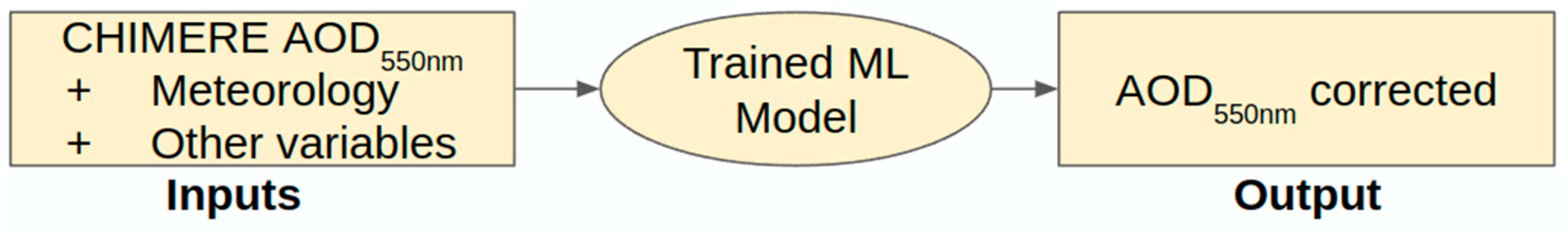
2.2. Bias Correction ML Models Construction

The fitting problem we are trying to solve is overdetermined and the high dimensional input variables are not independent. We implement several machine learning approaches, tree based, a neural network model, and the more classical linear regression model. In the following sections, we describe how the four models are built (Section 2.2.1, Section 2.2.2, Section 2.2.3 and Section 2.2.4) using the Python programming language version 3.8 [48] and the web-based interactive computing environment Jupyter notebook [49]. While training is partially performed on a Quadro P620 GPU, inference runs only on a single thread of a CPU (i9 2.30 GHz). The time required for training and inference of the ML models is an important indicator of the usability of the developed method. The training phases are relatively short; in fact, the multiple linear regression takes a few seconds, and the training of the other ML models does not exceed one hour each (not counting the hyperparameter search step, which is much longer). Regarding the inference time, all approaches perform the daily correction of the AOD in less than half a second (Table 1), which allows for a potential use of these models in real-time applications.

2.2.1. Multiple Linear Regression (MLR)

Multiple linear regression modeling is widely used in several fields because of its simplicity and its ease of use and interpretation. While it is more appropriate when the variables are independent, we tested it here to serve as a performance baseline and compare it to the three other more sophisticated ML models. Training is performed on half of randomly sampled DTrain data to keep the comparison fair with respect to the other ML models, which also use sampled data during a tuning phase.
If F is the function that maps the input features X to the output denoted by y, our goal is to find a function G that approximates F using a set of known solutions {Xi,yi}iN. Typically, the function is learned successively by minimizing the expected value of a loss function L(y, G(X)). The residuals are assumed to be normally distributed with constant variance. Given these assumptions and the fact that F is linear, we approximate it as the following Equation (1):
y   =   β 0 + β 1 X 1 + β 2 X 2 + .   .   . + β n X n + ε
where ε represents the error associated with the approximation, β0 is the intercept, βi is the regression coefficient corresponding to the feature Xi, where i is the feature order, and n the total number of the input features, which is 96 in our case.
The cost function L (Equations (2) and (3)) is below, which represents the residuals from the model and the observation is solved using the least squares method.
L   = j = 1 N y j y j 2
= j = 1 N y j β 0 i = 1 n β i X i , j 2
where N is the number of the observations available, and y i is the prediction of the multiple linear regression model for the feature of order i. For this work, we use its implementation in the sklearn v1.0.2 library [50].

2.2.2. Feed-Forward Neural Networks (NN)

Neural network regression is a modeling technique that is increasingly being used in many fields, thanks to the advancement of big data and parallelized hardware. The principle is to use perceptrons that are stacked in layers to approximate a non-linear relationship [51], where the weight of each perceptron is learned from a reference dataset by gradient backpropagation [47,52,53]. The technique can model non-linear relationships by using some activation functions [54]. Optimizing multi-dimensional functions with neural networks is difficult because of the proliferation of saddle points [55], but stochastic gradient descent algorithms are good at finding the global minimum [56,57,58].
Training of the NN AOD bias corrector is performed using the Tensorflow library v2.5.0 [59]. First, we search for a suitable network architecture for the problem by running 100 trials of feed-forward neural networks with dense layers. The architectures are sampled from an arbitrary reasonable hyperparameter search space (Supplementary Materials, Table S1). We use the random search tool of the Keras-tuner 1.0.3 library [60] to find the best network. All the tested networks use batch-normalized input feed [61] and a rectified linear unit [62] as the activation function. The use of a dropout layer [63,64] degrades the accuracy so we do not use it here. The weights of the network are optimized using the Adam optimizer [65], which is a variant of stochastic gradient descent, with respect to the mean squared error. The training is performed for 100 epochs, we set early stopping in the conditions when the validation loss either exceeds 0.1 or stabilizes at 0.01. We notice that increasing in the number of neurons (perceptrons) does not improve the accuracy of the estimator. Knowing that the architecture search is not exhaustive, we manage to obtain the same performance as the best randomly generated NN model using a bottleneck architecture, with less complexity and fewer parameters (Supplementary Materials, Table S2). The network has 3943 trainable parameters.

2.2.3. Random Forest (RF)

A random forest regressor [66] is an ensemble model that is widely used in both classification and regression problems. Each member of the ensemble, called a tree [67], is constructed using different randomized parameters. The final prediction is the average of the predictions of all the trees (forest).
The model is tuned for three key hyperparameters: number of estimators (trees), minimum samples in a leaf, and maximum number of features. The tuning is performed using the brute-force search method with two cross-fold validations on 10,000 randomly selected ground pixel data from DTrain. Using only a subset of the available training dataset speeds up the search process and saves memory. We find out that the best performing RF candidate has a maximum of 20 features, a minimum of 4 samples in leaf, and 100 estimators. We then train the best model using half of DTrain. The training was performed using scikit-learn v1.0.2.

2.2.4. Gradient Boosting (XGB)

A gradient boosting regressor [68,69] is also a tree-based modeling technique, but it constructs trees successively in such a way that each tree minimizes the residuals of the preceding trees. The final estimate is the sum of predictions of all the trees.
We use the Tree-based Pipeline Optimization Tool (TPOT) library v0.11.7. It is a genetic programming-based automated ML system that optimizes a set of feature preprocessors and ML models to build a better data processing pipeline for supervised tasks [70]. We let TPOT determine the best pipeline for correcting the CHIMERE AOD using 10,000 randomly selected data from DTrain. The number of generations is set empirically to 20 and the population size is set to 20, because further increasing these numbers slows down the search process. The best pipeline suggested by TPOT added the zeros and non-zero counts to the input features, and uses the XGBoost model (XGB) [69], which is a variation of the gradient boost model that uses L1 and L2 regularization. The XGB post-processor consists of 100 estimators, with a maximum depth of 9 and a minimum child weight of 17 (see the documentation [71] for more details on the meaning of these hyperparameters). The best pipeline proposed by TPOT is retrained using half of the DTrain dataset and is randomly sampled.

3. Results and Discussion

In this section, we analyze the performance of the trained AOD bias correctors on DTest against the MODIS observations. First, we detail a case study (a in Section 3.1) where we investigate the influence of the input features on the predicted AOD. We discuss the statistical performance of the ML models in b in Section 3.1, then present a use case of the AOD correction at a time of the day that is different from the one used for training the ML models (c in Section 3.1). Finally, we present a comparison against ground-based AERONET measurements (Section 3.2).

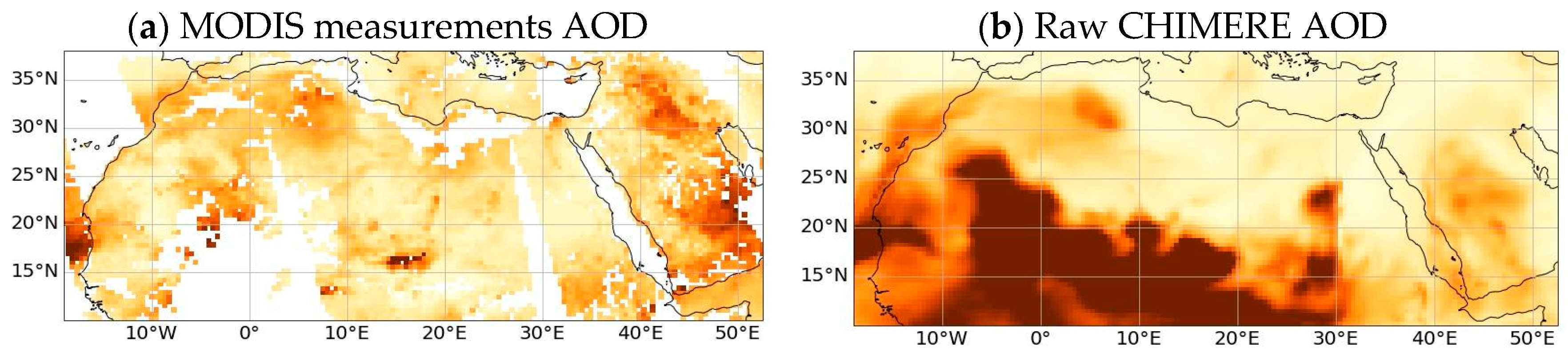
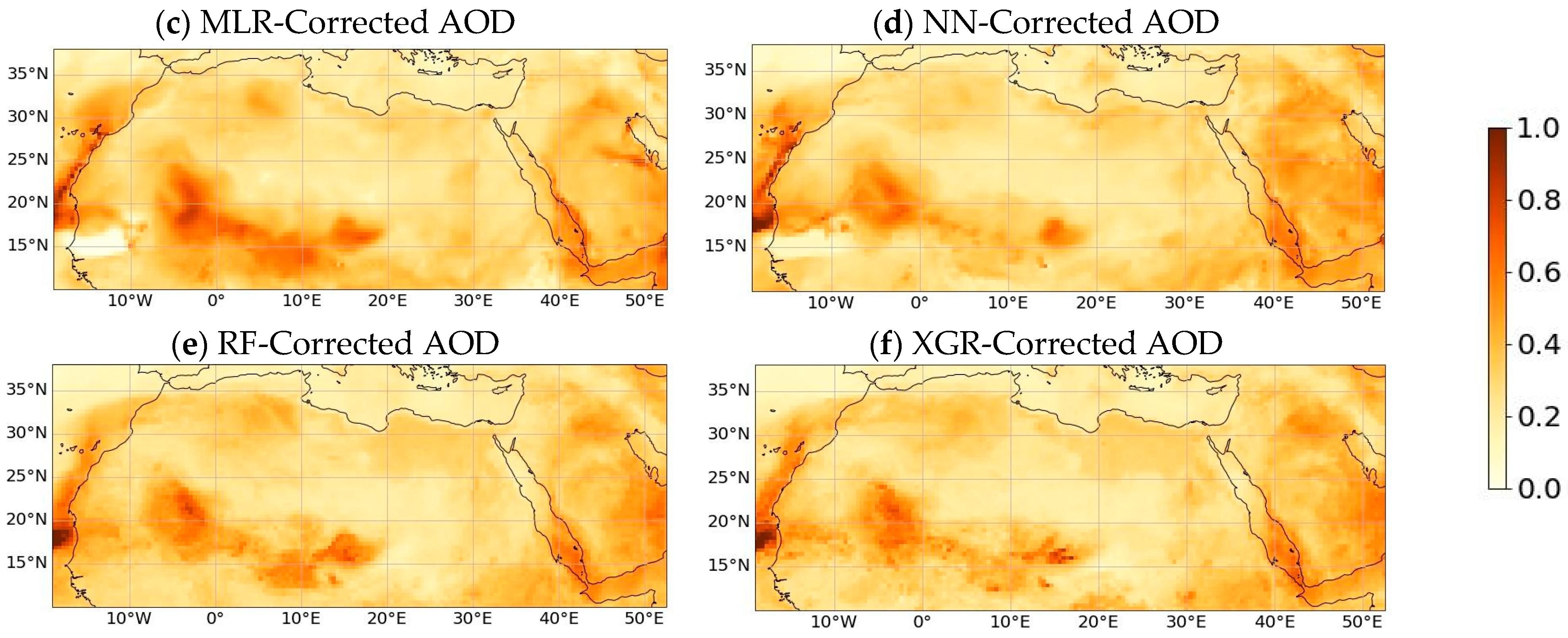
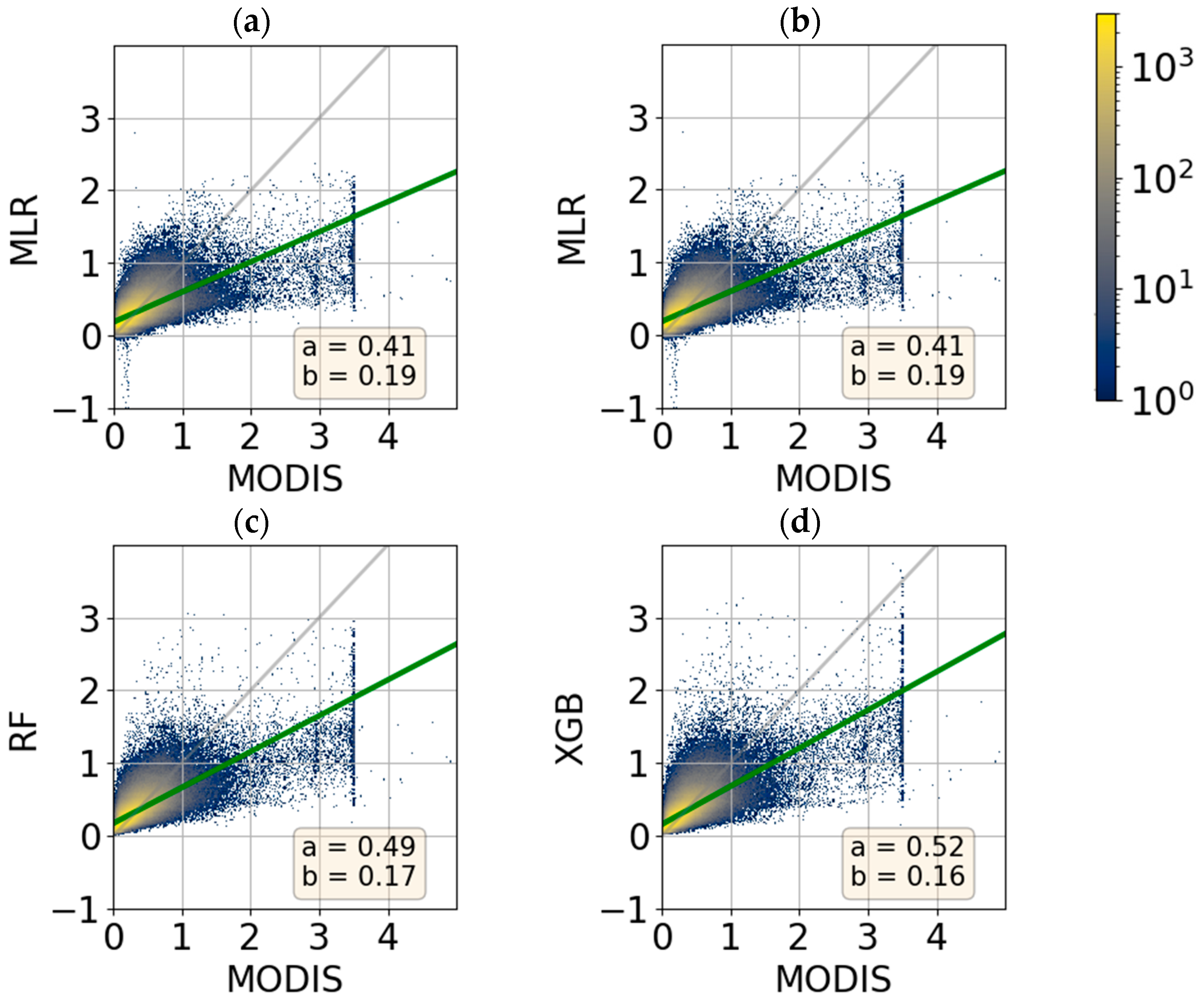
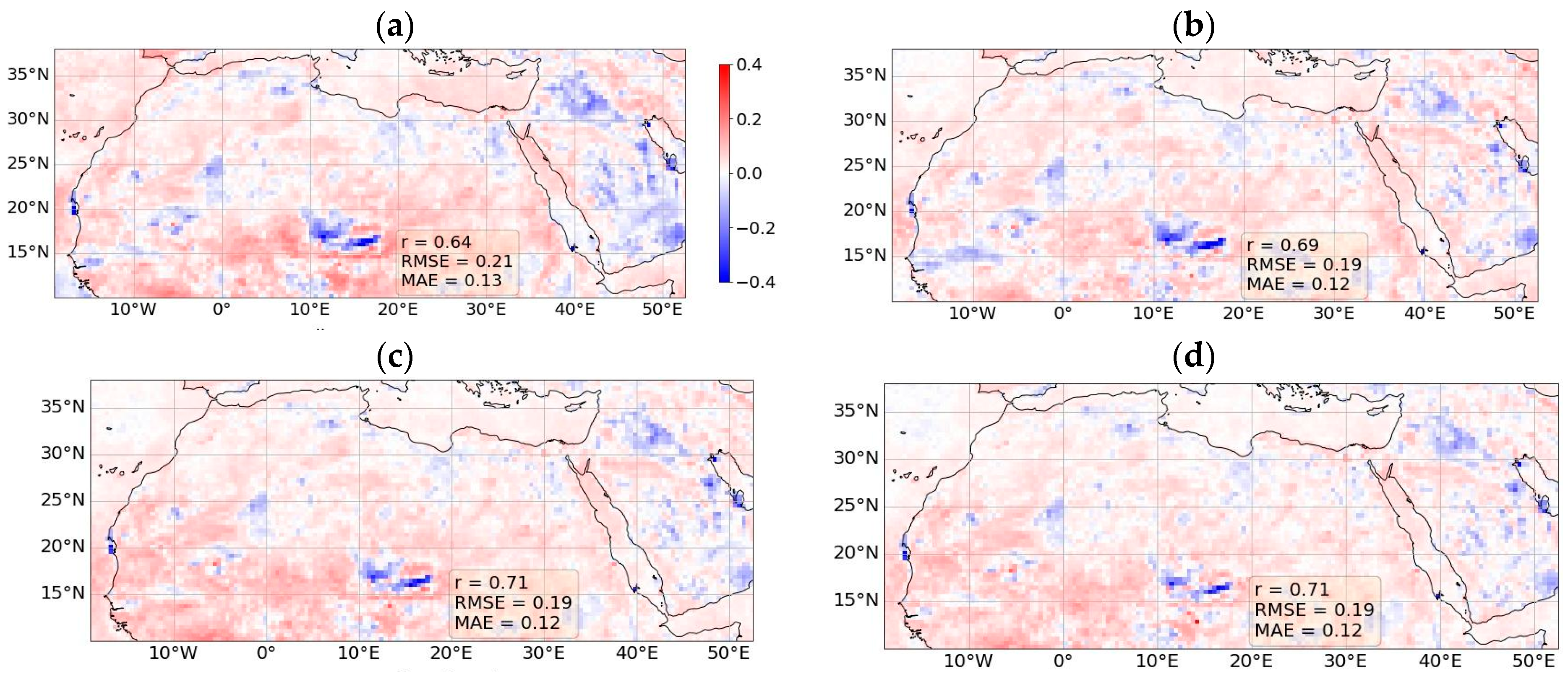
3.1. Comparison against Independent MODIS Observations

a.
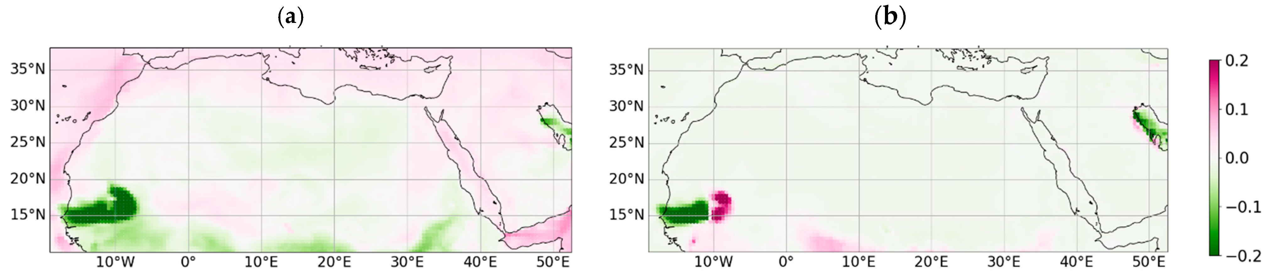
Case study of 30 September 2021
The bias-corrected AODs predicted with the four ML models (Figure 4c–f) are compared with the MODIS AOD measurements (Figure 4a) and with the CHIMERE raw (uncorrected) AOD simulations (Figure 4b) for the case study of 30 September 2021. This event is characterized by a large desert dust outbreak originating from the southern border of the Sahara (as typically observed during summertime in this region, e.g., [72]), and anthropogenic pollution fine particles located over the southeastern part of the Arabian Peninsula. This is consistently shown by CHIMERE simulation and also by the aerosol Ångström exponent values derived from MODIS AQUA Deep Blue (maps available in the Worldview portal [73]). As expected, the latter are close to zero over the Sahara, which is typical for coarse particles such as desert dust, but they are significantly higher (about 1.8) over the AOD patches over the Arabian Peninsula, thus suggesting the presence of fine particles as those of anthropogenic origin.
Compared to the satellite data, the corrected AOD maps predicted by the ML models provide a clear added value with their full geographic coverage. They are not affected by the cloud cover or the satellite swath size, while offering better accuracy than the raw CHIMERE simulations. The ML models successfully corrected the AOD by reducing the raw CHIMERE values in the high desert dust load regions such as the Southern, Central, and Western Sahara. Additionally, they increase the low AOD values over the northern and southern Arabian Peninsula that are underestimated by CHIMERE. This significantly improves the agreement with respect to MODIS measurements. Despite the independent pixel-by-pixel processing of the ML approaches, the horizontal structures of the corrected AOD features are continuous and homogeneous in most of the regions. This is true for most of the dates of the DTest dates. There are exceptions, such as some horizontal discontinuities seen near the southwest coast of North Africa on 30 September 2021 from the NN and MLR predictions (Figure 4c,d). According to MODIS observations, these discontinuities in the AOD do not reflect the natural concentration gradient found in these dust plumes. In the case of MLR (Figure 4c), the issue could be associated with the use of negative regression coefficients. For the NN model, the problem might be explained by the fact that multi-layer perceptrons may not extrapolate well the non-linear relationships outside the training set [74]. In fact, its low performance has also been observed in another model’s inter-comparison work [20]. The XGB and RF bias correctors do not show such artifacts (Figure 4e,f). However, we note that XGB is slightly noisier, suggesting an overfit to the MODIS AOD pixel noise. In fact, Breiman suggests that using a random selection of features to split each node in tree-based models yields error rates that are comparable to adaptive boosting (Adaboost) but more robust to noise [66].
Additional analyses of the performance of the ML approaches are provided by feature importance values (Figure 5, Figure 6 and Figure 7) computed using the Shapley Additive exPlanations (SHAP) framework [75]. Shapley values are commonly used in cooperative game theory to fairly determine each player’s contribution to the total payoff, taking into account all the possible coalitions of players. In our study, they allow us to the investigate the source of the spatial artifacts and help us understand which input features are the most important and how they spatially affect the prediction of the ML models. These values are computed considering all the possible combinations of the input features while estimating the marginal contribution (either positive or negative) of each one of them to the model output. Input features of 3D variable fields are vertically summed up to obtain the contribution of the actual geophysical variable, rather than a unique feature (for each individual altitude). All of these calculations are quite computationally costly. Therefore, the following variable importance analysis is limited to the test case of 30 September 2021.
Figure 5 shows the horizontally averaged absolute contribution of each input variable for the four ML models in terms of Shapley values. It shows that a larger number of variables contribute relatively evenly to the prediction of the AOD values for the RF and XGB models than those of MLR and NN. For the latter, some variables, such as the abundance of ammonium particles and OH radicals, show almost zero importance. For all ML models, as expected, the raw CHIMERE AOD is important for the predictions, and in the case of RF, this is also true for other variables that also represent the abundance of aerosols, such as particle mass concentrations in terms of PM2.5, PM10, and total dust concentration. Another important variable for all the ML models is the specific humidity, especially for the MLR model, where three humidity-related variables share half of the total prediction importance. As noted in the following paragraph, the ML models appear to use humidity to numerically adjust the background values of AODs in different ways over either dry or humid regions. In the case of RF and XGB, moderate importance is also seen for meteorological variables (such as atmospheric pressure, shortwave radiation, sensible heat flux, and water droplet precipitation) and also for atmospheric species related to anthropogenic activities and chemically active species, such as nitrate, sulfate particles, and OH. The latter suggests a potential ability of the two ML models mentioned above to account for contrasting meteorological conditions on aerosol evolution (e.g., clear skies during high-pressure situations or the influence of low-pressure systems with increasing cloudiness) and the influence of anthropogenic emissions on particle abundances (the geographical influence of the latter is discussed in the following paragraphs).
The horizontal distribution of the Shapley values is very valuable for explaining the role of each input feature in correcting the AOD (see Figure 6 and Figure 7 for, respectively, RF and MLR models). Shapely maps for the CHIMERE raw AODs show that this feature is used to modulate the AOD in the regions affected by the desert dust outbreak in the central Sahara (see the very intense reddish values in Figure 6a). A similar use is expected for the PM10 variable, but with some local differences (such as over northern part of the Sahara) and a more moderate intensity (Figure 6c). The map of Shapley values for the specific humidity shows a quite different structure, with significant and negative values north of 20°N. Over northeast Africa, this region is dry and shows rather low values of desert dust AODs, which are underestimated by CHIMERE (see Figure 4a,b). We suggest that the ML models may use these co-located conditions as a corrector for these background values of desert dust AOD (see the correction of this bias in Figure 4c–f).
Another very interesting aspect is highlighted by the Shapley values for nitrate particles (Figure 6d). We notice that their most important influence is located over the Arabian Peninsula, collocated with the anthropogenic particle event prevailing over this region. Interestingly, we clearly see that the ML models (especially RF and XGB, Figure 4c–f) can adequately correct this negative bias of the raw simulation’s AOD, which is related to particles of a different origin (anthropogenic activity) as over North Africa, and appropriately use the nitrate particle concentration for its prediction.
Furthermore, the artifacts of sharp variations of the AOD with very low values over southwestern part of the Sahara for the MLR and NN model predictions (Figure 4c,d) can also be explained by the SHAP analysis (Figure 7). It shows that two variables are responsible for this artifact, the hydroperoxide radical and the non-methane hydrocarbon concentrations (Figure 7 for MLR). The negative contribution of these two variables in the region around 10°W, 15°N dominates the overall prediction of the AOD, leading to the abnormally low values (Figure 4c,d). This is not observed for RF and XGB.
b.
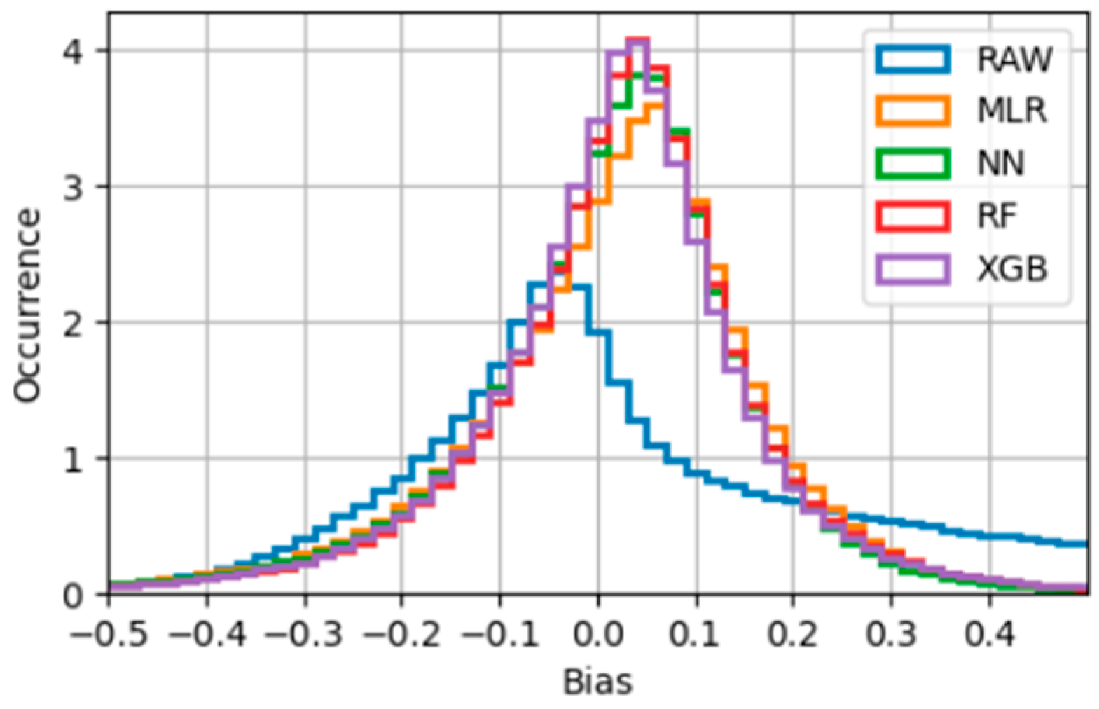
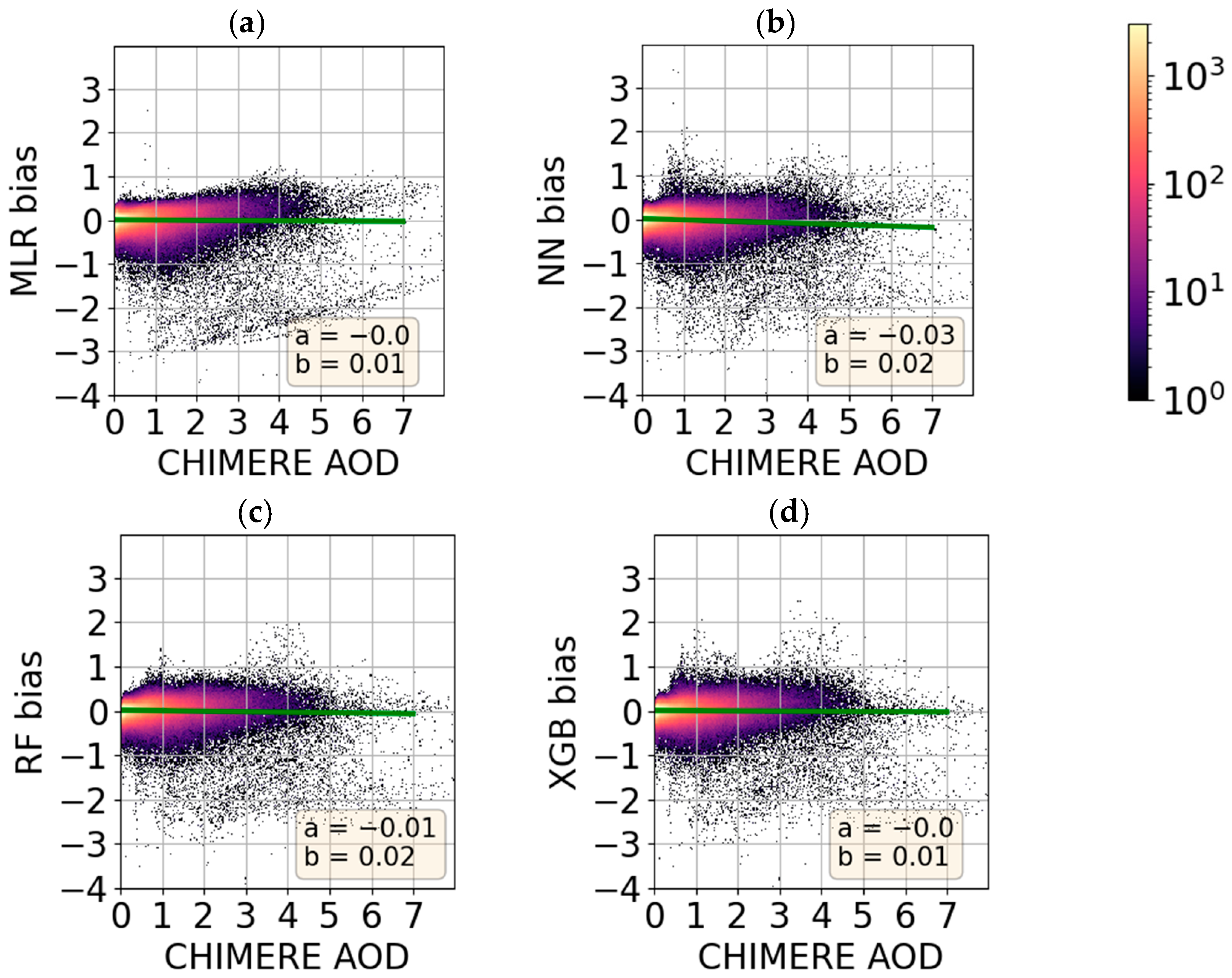
Statistical analysis on the testing dataset
For the entire DTest dataset in 2021, we compare the estimates of the raw AOD CHIMERE simulation and the inferences from the ML models with respect to the MODIS observations that are not used in the training phase (Table 1). The table shows that the ML models successfully correct the raw CHIMERE AODs in a statistically consistent and stable manner throughout the year 2021. They all show a comparable improvement in AOD correction, with both larger correlation coefficients r with MODIS AOD (r between 0.62 and 0.71) and smaller RMSE (from 0.19 to 0.21) and MAE. The improvement in AOD estimation is clearly evident when comparing to the raw CHIMERE AODs performance (r value of 0.56 and RMSE of 0.65). We note that the XGB and RF are the best-performing bias correctors in terms of the correlation coefficient (0.71) and RMSE (0.19). The NN model follows with the same RMSE but a slightly lower correlation coefficient (0.69). Finally, the MLR corrector offers a slightly lower correlation coefficient (0.62) and a higher RMSE (0.21).
The AOD correction biases (with respect to MODIS observations) show frequency histograms that are bell-shaped and centered around a small positive value. This suggests a small overall positive overcorrection of the raw AOD (Figure 8). This is consistent with the positive values of the medians (50% percentile) and the negative skewness in Table 1. On the other hand, the mean bias values (μ) are close to or equal to zero, which is expected since the models are trained by minimizing the mean squared error.
The model bias ranges are also quite similar. The minimum bias is rather similar for all ML models (between −4.21 and −3.96). The maximum bias values on the other hand, which correspond to the extreme underestimation of the AOD, come from the NN model with a maximum bias of 5.09; while the best model in terms of underestimation is the RF model with a maximum bias of 2.
We observe that the distributions of the AOD bias corrections of CHIMERE (Figure 8) are skewed toward higher values. This is because there are more background AOD pixels that are underestimated by CHIMEREs raw AODs, while they are overestimated for the high AOD episodes. The overestimation occurs in most of the dust emission episodes with very large bias values, as shown in Figure 3, which is why the bias RMSE is high, and the median bias is positive (0.03) in Table 1.
According to the RF and XGB models, the most important input feature is the CHIMERE raw AOD (Figure 5). Therefore, it is interesting to compare the correction versus the a priori (CHIMERE raw) AOD, which indicates the relationship between the a priori AOD in terms of intensities on the predicted AOD. The bias in the AOD correction of the different ML models is found to be only slightly dependent on the a priori AOD values (Figure 9). For all of them, we observe that for high a priori AODs (above a 0.5 value), the correction can be significant. While for low a priori values, the AODs correction is more limited, suggesting low bias for raw CHIMERE AODs typically under 0.3 (in the majority of the pixels). This may be attributed to the fact that there are more pixels available for training with a typically low background AOD level. The same model behavior was observed in previous research [20].
The analysis of the predicted AOD of the different ML models varies according to the AOD level (Figure 10). For low AOD levels (below 1), the models mostly correct the AOD of CHIMERE to an acceptable degree (yellow colors), with a slightly insufficient correction for higher AOD levels. The MLR model (Figure 10a) infers negative AODs for some pixels. This is an artifact (see also Figure 4c) that is associated with the use of negative regression coefficients, which improves the overall performance (r) of the MLR model. In these terms, the best performing ML model is the XGB (Figure 10d) with a linear fit slope of 0.52, followed by the RF model.
Figure 11 shows an evaluation of the performance of the four ML-based bias correctors in terms of the median bias of the AOD correction over the entire test dataset, DTest. The median bias does not exceed 0.3 in most of the domain, and it is significantly smaller than that of the raw CHIMERE simulations (Figure 3). Similar biases are seen for the four correctors, with some positive and some negative biases for several regions characterized by high annual mean AOD values (Supplementary Material, Figure S1b), and they are smaller in absolute terms for RF and XGB, especially over the Arabian Peninsula and the southwestern part of the Sahara. A common behavior of all the ML models is that they strongly underestimate the AOD over a zone (10° to 20°E, 14° to 20°N) corresponding to the Bodélé Depression (Figure 11).
The Bodélé Depression region is known to be a major source of desert dust [46]. The region is part of the former paleolake Megachad, which was the largest lake on the planet 7000 years ago [76]. Mineral dust emissions from the Bodélé Depression region are generally relatively fine-grained coarse dusts dominated by quartz, with admixtures of clay minerals and Fe oxyhydrates [77]. Therefore, they are brighter (higher reflectance) and whiter (flat reflectance spectrum), compared to the rest of the Saharan plumes [78] (Supplementary Materials, Figure S1a). Indeed, Algerian Saharan dust [79] and the Bodélé Depression region dust [80] have different refractive indices. In contrast to the CHIMERE CTM model, the aerosol retrieval algorithm Deep Blue uses two different single scattering albedos for the dust AOD retrieval [78], one for the redder dust, and one for the whiter dust. Furthermore, an upper limit of 3.5 is set for the AOD values derived from the MODIS AQUA operational algorithm [22].
These remarks suggest that potential improvements in the representation of the particle optical properties and the size within CHIMERE, along with the accuracy of the near-surface wind speeds responsible for the dust uplift, could reduce the bias in the simulated AOD in North Africa. However, this is beyond the scope of this paper.
c.
Prediction of bias corrected AODs at the different daytimes
The AOD correction models are trained using MODIS AQUA satellite observations, which has an overpass time of (13:30 LT). It is necessary to ensure that the models are temporally stable and usable outside the AQUA overpass time. For this purpose, we correct the raw CHIMERE AOD outputs at 10:00 LT using the RF model, and then compare the inferred AODs to MODIS observations from the Terra satellite, which has a local overpass time of 10:30 LT. Thus, the daytime of the training database (13:30 LT) is different from that of the test (10:30 LT). We chose only the RF model to perform the upcoming analysis because the statistical performance of the other ML models is similar. The comparison shows that improvement in correlation and residuals is comparable to the corrected AODs at 13:00 LT. From Table 2, we can see that the residuals (RMSE, MAE, and MB) are improved. The RMSE is reduced by 0.68% and the correlation is increased to 0.68 (from 0.52 for the raw CHIMERE AODs). This good AOD correction for a morning hour implies the possibility of using the correction method for different simulation hours of the day. However, we remain conservative in using the AOD correction method during night hours as the ML model will more often have to extrapolate unseen situations, e.g., low boundary layer heights, low temperatures, etc.

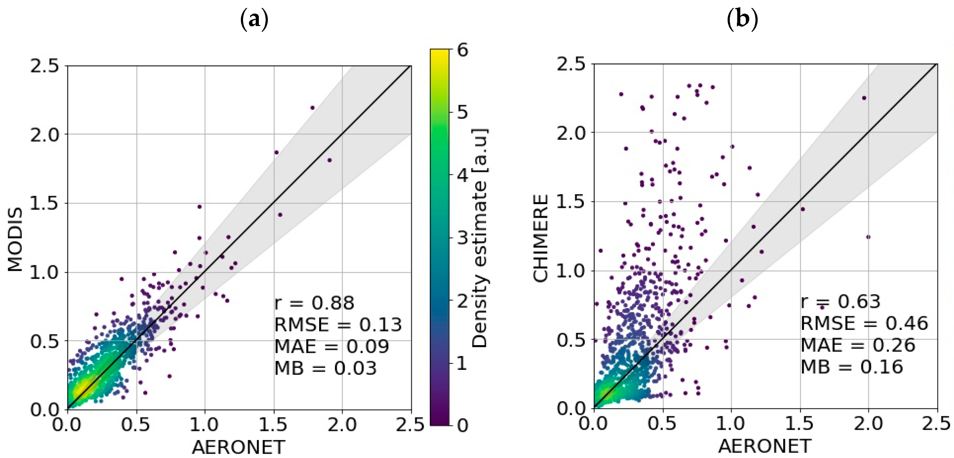
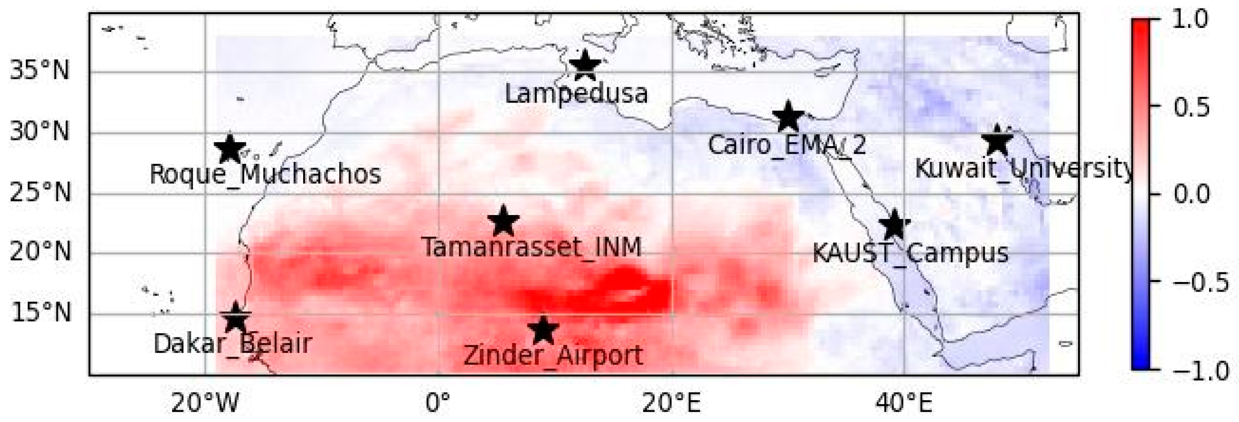
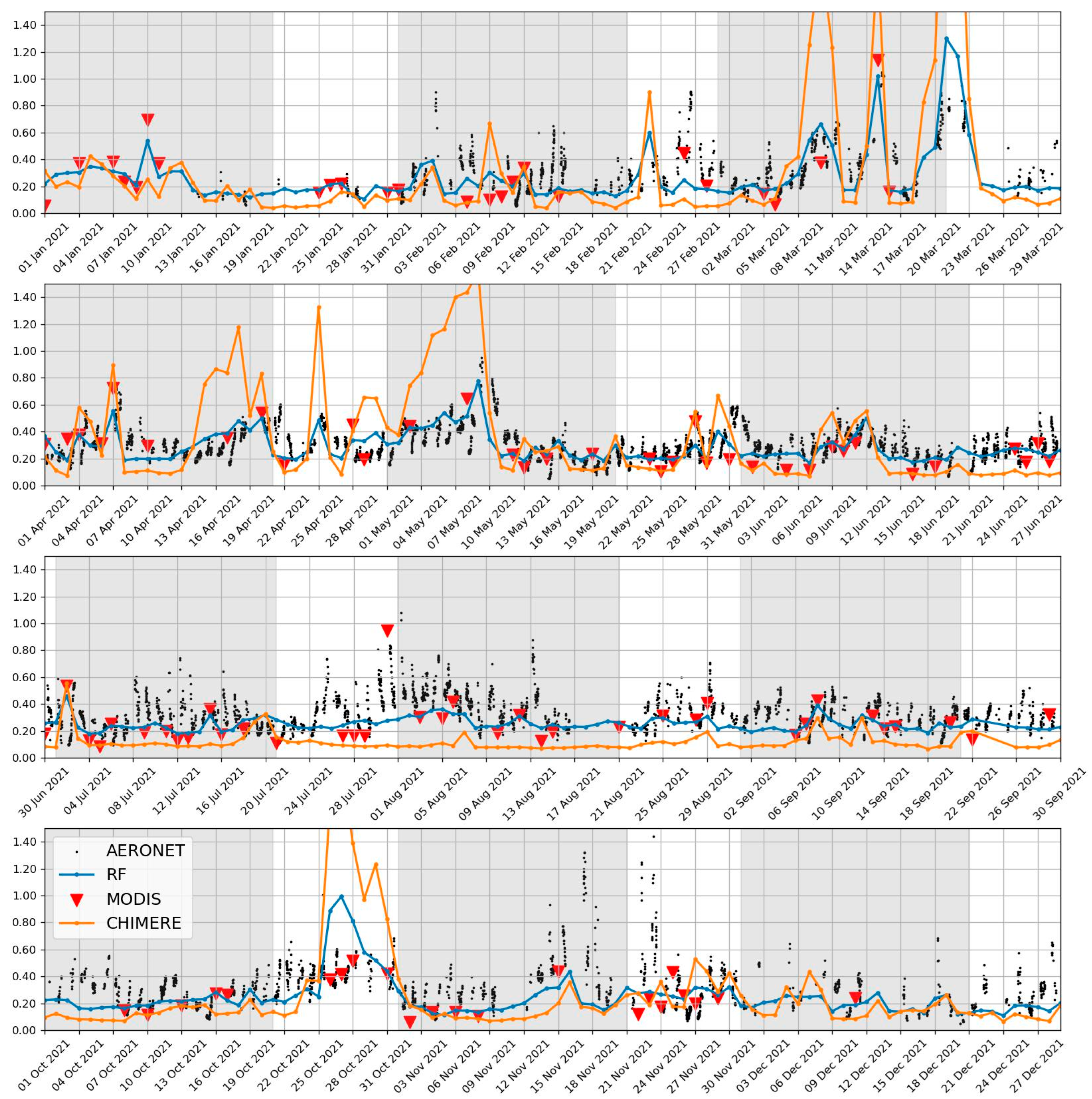
3.2. Comparison with AERONET Ground-Based Measurements

The performance of the RF model together with that of MODIS is assessed against the collocated AERONET measurements at the eight stations for test dates (Table 3). We see an improvement in the correlation coefficient r to 0.73 (from 0.54 for the raw AOD). The residuals also improve as the RMSE and MAE decrease from 0.45 and 0.27 to about 0.16 and 0.12, respectively. The MB is significantly reduced from 0.18 to about 0.6 for the corrected AOD.
Figure 12 illustrates the daily evolution and temporal consistency of the performance of the RF model. It is worth noting that for visual completeness, the figure also shows comparisons for the days used in the training phase (in the gray background), but we limit the analysis to the test dates (in the white background). We chose the measurement time series from the station of Cairo for this purpose because of its good data coverage of the period and because it shows situations of positive and negative corrections of the biases, with desert dust and anthropogenic aerosol events (the same kind of figures for other sites can be found at the link in the data availability clause). A number of high AOD episodes are seen in March and April and from 24 to 29 October 2021. In these cases, the raw AODs simulated by CHIMERE (orange lines) are clearly overestimated with respect to the AERONET measurements (black lines). The ML-based corrector reduces the AOD values (blue lines) to clearly approach the sun photometer measurements, while still depicting the AOD peaks.
On the other hand, CHIMERE simulations underestimate the AOD during the periods of 20–27 June and 21 to 30 September. These periods are characterized by background anthropogenic pollution, as suggested by co-located relatively high aerosol Angstrom exponents (around 1.8) measured by MODIS AQUA (seen in the Worldview portal, not shown). In this case, the ML-corrected AODs are successfully improved to reach values that are closer to both AERONET and MODIS measurements (red triangles). Moreover, in cases of rather correct raw CHIMERE AODs (e.g., on 20–21 May), the ML-derived bias corrector does not modify the AOD, which remains around 0.24.

4. Conclusions

In this work, we develop a new ML-based model to significantly improve the accuracy of AOD maps, initially derived from CHIMERE chemistry transport model simulations. The ML model is trained with MODIS satellite measurements, which are not used in the inference stage. This approach provides full-coverage daily maps of AODs over North Africa and the Arabian Peninsula with a clearly better agreement with respect to satellite and ground-based observations as compared to AODs from raw, uncorrected CHIMERE simulations. The AODs corrected by the ML models show substantially higher correlations and lower errors (RMSE and MAE) than the raw AOD simulations, as compared to MODIS satellite measurements. The RMSE of the AODs is reduced from 0.65 (raw CHIMERE) to 0.19 (RF bias corrector), and the correlation coefficient r is increased from 0.56 to 0.71 (respectively, for raw CHIMERE and the RF corrector). The bias corrector reduces the overestimation in the AOD maps over the Saharan desert and the underestimation over the Arabian Peninsula. This is performed not only for desert dust during outbreaks and background conditions, but also for anthropogenic pollution aerosols. However, a slight overestimation of the correction is observed at low aerosol loads.
The spatially continuous AOD correction could potentially be used as a gap-filling system for the global MODIS AOD observations. Additionally, this current accomplishment suggests the possibility of using advanced retrievals of the 3D distribution of aerosols such as AEROIASI [81], and AEROS5P [82], which utilize Infrared Atmospheric Sounding Interferometer (IASI) thermal infrared measurements for coarse particles and TROPospheric Ozone Monitoring Instrument (TROPOMI) measurements for fine particles, respectively, to correct the CHIMERE vertical profile of aerosol concentrations.
Among the four ML-based bias correctors, the best results are found for the RF regressor, which gives a spatially smooth AOD in good agreement with MODIS AODs. The other bias correctors used here (MLR, XGB, and NN) also improve the accuracy of the AOD, but show spatial artifacts, some of them related to overfitting. The AOD correction was tested for a different time of the day than the one used for the training. The comparison of the CHIMERE AOD correction at 10:00 LT with that of MODIS Terra, which has a close overpass time (10:30 LT), shows that the RF model also provides good results even for this time of the day, which is different from that of the training dataset. This is a step toward validating the AOD correction for any daytime application of the CHIMERE simulation.
Evaluation of the daily consistency of the corrected AOD shows that the overestimation of peaks and the underestimation of background values at a given location (shown for Cairo) have been successfully improved, for both desert dust and anthropogenic aerosol loads. These results are consistent with analyses of the influence of the input features, showing that the RF model adequately uses different atmospheric constituents to deal with different situation (e.g., desert dust, anthropogenic pollution, and background concentrations). We also find that the ML-derived AODs may still underestimate very high AOD values compared to MODIS observations.
In this study, ML models are implemented with CHIMERE simulations that are performed with meteorological analysis data. Therefore, the AOD correction applied to CHIMERE simulations using meteorological forecasts may be less accurate. Adjustments to the ML models may be required. Furthermore, a deep understanding of the contribution of different features will help to improve the temporal stability and reduce the spatial artifacts.

Supplementary Materials

The following supporting information can be downloaded at: https://www.mdpi.com/article/10.3390/rs15061510/s1.

Author Contributions

Conceptualization, formal analysis, methodology, data curation, software, visualization, validation, writing—original draft, F.L.; conceptualization, funding acquisition, project administration, supervision, writing—review and editing, J.C.; data curation, writing—review and editing, M.L.; methodology, writing—review and editing, J.B.; methodology, writing—review, A.C.; writing—review and editing, M.B.; funding acquisition, writing —review, C.D. All authors participated in the analysis. All authors have read and agreed to the published version of the manuscript.

Funding

This work is funded by the Region Ile-de-France in the framework of the Domaine d’Intérêt Majeur Réseau de recherche Qualité de l’air en Ile-de-France (DIM QI2) through the program Paris Region PhD (PRPHD) and ARIA Technologies, and is supported by the Centre National d’Études Spatiales (CNES) through the SURVEYPOLLUTION project from TOSCA (Terre Ocean Surface Continental et Atmosphère), the Centre National de Recherche Scientifique—Institute National de Sciences de l’Univers (CNRS-INSU), and the Université Paris Est Créteil (UPEC).

Data Availability Statement

In this link, shorturl.at/oLY28, several materials can be requested, including additional AOD maps figures, the data results and those used for the development of this work, in addition to the trained ML models.

Acknowledgments

We thank the DIM Qi2 of Ile-de-France region for funding this study. We are grateful to the CNES (SURVEYPOLLUTION/TOSCA project), and to ARIA Technologies for the financial support. We acknowledge the free use of NASA’s Earth Observing System Data and Information System (EOSDIS). We also acknowledge the free use of the open-source Python software and libraries. We thank the developers of the CHIMERE chemistry-transport model from LMD and LISA laboratories. We also thank the staff of the (8) AERONET stations used in this work for establishing and maintaining the sites. Finally, we thank the anonymous reviewers for their constructive comments and suggestions, which helped to improve the quality of this manuscript.

Conflicts of Interest

The authors declare no conflict of interest.

References

  1. Tsikerdekis, A.; Zanis, P.; Georgoulias, A.K.; Alexandri, G.; Katragkou, E.; Karacostas, T.; Solmon, F. Direct and Semi-Direct Radiative Effect of North African Dust in Present and Future Regional Climate Simulations. Clim. Dyn. 2019, 53, 4311–4336. [Google Scholar] [CrossRef]
  2. Mahowald, N.M.; Baker, A.R.; Bergametti, G.; Brooks, N.; Duce, R.A.; Jickells, T.D.; Kubilay, N.; Prospero, J.M.; Tegen, I. Atmospheric Global Dust Cycle and Iron Inputs to the Ocean. Glob. Biogeochem. Cycles 2005, 19, GB4025. [Google Scholar] [CrossRef]
  3. Klingmüller, K.; Lelieveld, J.; Karydis, V.A.; Stenchikov, G.L. Direct Radiative Effect of Dust–Pollution Interactions. Atmos. Chem. Phys. 2019, 19, 7397–7408. [Google Scholar] [CrossRef] [Green Version]
  4. Meng, L.; Zhao, T.; He, Q.; Yang, X.; Mamtimin, A.; Wang, M.; Pan, H.; Huo, W.; Yang, F.; Zhou, C. Dust Radiative Effect Characteristics during a Typical Springtime Dust Storm with Persistent Floating Dust in the Tarim Basin, Northwest China. Remote Sens. 2022, 14, 1167. [Google Scholar] [CrossRef]
  5. Lelieveld, J.; Evans, J.S.; Fnais, M.; Giannadaki, D.; Pozzer, A. The Contribution of Outdoor Air Pollution Sources to Premature Mortality on a Global Scale. Nature 2015, 525, 367–371. [Google Scholar] [CrossRef] [PubMed]
  6. Remer, L.A.; Kaufman, Y.J.; Tanré, D.; Mattoo, S.; Chu, D.A.; Martins, J.V.; Li, R.-R.; Ichoku, C.; Levy, R.C.; Kleidman, R.G.; et al. The MODIS Aerosol Algorithm, Products, and Validation. J. Atmos. Sci. 2005, 62, 947–973. [Google Scholar] [CrossRef] [Green Version]
  7. Menut, L.; Bessagnet, B.; Briant, R.; Cholakian, A.; Couvidat, F.; Mailler, S.; Pennel, R.; Siour, G.; Tuccella, P.; Turquety, S.; et al. The CHIMERE V2020r1 Online Chemistry-Transport Model. Geosci. Model Dev. 2021, 14, 6781–6811. [Google Scholar] [CrossRef]
  8. Bessagnet, B.; Hodzic, A.; Vautard, R.; Beekmann, M.; Cheinet, S.; Honoré, C.; Liousse, C.; Rouil, L. Aerosol Modeling with CHIMERE—Preliminary Evaluation at the Continental Scale. Atmos. Environ. 2004, 38, 2803–2817. [Google Scholar] [CrossRef]
  9. Turquety, S.; Menut, L.; Siour, G.; Mailler, S.; Hadji-Lazaro, J.; George, M.; Clerbaux, C.; Hurtmans, D.; Coheur, P.-F. APIFLAME v2.0 Biomass Burning Emissions Model: Impact of Refined Input Parameters on Atmospheric Concentration in Portugal in Summer 2016. Geosci. Model Dev. 2020, 13, 2981–3009. [Google Scholar] [CrossRef]
  10. Mallet, V.; Sportisse, B. Uncertainty in a Chemistry-Transport Model Due to Physical Parameterizations and Numerical Approximations: An Ensemble Approach Applied to Ozone Modeling. J. Geophys. Res. 2006, 111, D01302. [Google Scholar] [CrossRef]
  11. Escribano, J.; Boucher, O.; Chevallier, F.; Huneeus, N. Impact of the Choice of the Satellite Aerosol Optical Depth Product in a Sub-Regional Dust Emission Inversion. Atmos. Chem. Phys. 2017, 17, 7111–7126. [Google Scholar] [CrossRef] [Green Version]
  12. Escribano, J.; Boucher, O.; Chevallier, F.; Huneeus, N. Subregional Inversion of North African Dust Sources. J. Geophys. Res. D Atmos. 2016, 121, 8549–8566. [Google Scholar] [CrossRef] [Green Version]
  13. Garrigues, S.; Chimot, J.; Ades, M.; Inness, A.; Flemming, J.; Kipling, Z.; Benedetti, A.; Ribas, R.; Jafariserajehlou, S.; Fougnie, B.; et al. Monitoring Multiple Satellite Aerosol Optical Depth (AOD) Products within the Copernicus Atmosphere Monitoring Service (CAMS) Data Assimilation System. Atmos. Clim. Sci. 2022, 22, 14657–14692. [Google Scholar] [CrossRef]
  14. Bocquet, M.; Elbern, H.; Eskes, H.; Hirtl, M.; Žabkar, R.; Carmichael, G.R.; Flemming, J.; Inness, A.; Pagowski, M.; Pérez Camaño, J.L.; et al. Data Assimilation in Atmospheric Chemistry Models: Current Status and Future Prospects for Coupled Chemistry Meteorology Models. Atmos. Chem. Phys. 2015, 15, 5325–5358. [Google Scholar] [CrossRef] [Green Version]
  15. Sayeed, A.; Eslami, E.; Lops, Y.; Choi, Y. CMAQ-CNN: A New-Generation of Post-Processing Techniques for Chemical Transport Models Using Deep Neural Networks. Atmos. Environ. 2022, 273, 118961. [Google Scholar] [CrossRef]
  16. Xu, M.; Jin, J.; Wang, G.; Segers, A.; Deng, T.; Lin, H.X. Machine Learning Based Bias Correction for Numerical Chemical Transport Models. Atmos. Environ. 2021, 248, 118022. [Google Scholar] [CrossRef]
  17. Jin, J.; Lin, H.X.; Segers, A.; Xie, Y.; Heemink, A. Machine Learning for Observation Bias Correction with Application to Dust Storm Data Assimilation. Chem. Phys. Lipids 2019, 19, 10009–10026. [Google Scholar] [CrossRef] [Green Version]
  18. Rasp, S.; Lerch, S. Neural Networks for Postprocessing Ensemble Weather Forecasts. Mon. Weather Rev. 2018, 146, 3885–3900. [Google Scholar] [CrossRef] [Green Version]
  19. Taillardat, M.; Mestre, O.; Zamo, M.; Naveau, P. Calibrated Ensemble Forecasts Using Quantile Regression Forests and Ensemble Model Output Statistics. Mon. Weather Rev. 2016, 144, 2375–2393. [Google Scholar] [CrossRef]
  20. Nabavi, S.O.; Haimberger, L.; Abbasi, R.; Samimi, C. Prediction of Aerosol Optical Depth in West Asia Using Deterministic Models and Machine Learning Algorithms. Aeolian Res. 2018, 35, 69–84. [Google Scholar] [CrossRef]
  21. Available online: https://modis.gsfc.nasa.gov/about/specifications.php (accessed on 27 July 2022).
  22. Sayer, A.M.; Munchak, L.A.; Hsu, N.C.; Levy, R.C.; Bettenhausen, C.; Jeong, M.-J. MODIS Collection 6 Aerosol Products: Comparison between Aqua’s e-Deep Blue, Dark Target, and “Merged” Data Sets, and Usage Recommendations. J. Geophys. Res. 2014, 119, 13965–13989. [Google Scholar] [CrossRef]
  23. Wei, J.; Li, Z.; Peng, Y.; Sun, L. MODIS Collection 6.1 Aerosol Optical Depth Products over Land and Ocean: Validation and Comparison. Atmos. Environ. 2019, 201, 428–440. [Google Scholar] [CrossRef]
  24. Gupta, P.; Levy, R.C.; Mattoo, S.; Remer, L.A.; Munchak, L.A. A Surface Reflectance Scheme for Retrieving Aerosol Optical Depth over Urban Surfaces in MODIS Dark Target Retrieval Algorithm. Atmos. Clim. Sci. 2016, 9, 3293–3308. [Google Scholar] [CrossRef] [Green Version]
  25. Hsu, N.C.; Jeong, M.-J.; Bettenhausen, C.; Sayer, A.M.; Hansell, R.; Seftor, C.S.; Huang, J.; Tsay, S.-C. Enhanced Deep Blue Aerosol Retrieval Algorithm: The Second Generation. J. Geophys. Res. 2013, 118, 9296–9315. [Google Scholar] [CrossRef]
  26. Holben, B.N.; Eck, T.F.; Slutsker, I.; Tanré, D.; Buis, J.P.; Setzer, A.; Vermote, E.; Reagan, J.A.; Kaufman, Y.J.; Nakajima, T.; et al. AERONET—A Federated Instrument Network and Data Archive for Aerosol Characterization. Remote Sens. Environ. 1998, 66, 1–16. [Google Scholar] [CrossRef]
  27. Menut, L.; Bessagnet, B.; Khvorostyanov, D.; Beekmann, M.; Blond, N.; Colette, A.; Coll, I.; Curci, G.; Foret, G.; Hodzic, A.; et al. CHIMERE 2013: A Model for Regional Atmospheric Composition Modelling. Geosci. Model Dev. 2013, 6, 981–1028. [Google Scholar] [CrossRef] [Green Version]
  28. Available online: http://www.prevair.org/ (accessed on 27 July 2022).
  29. Ciarelli, G.; Theobald, M.R.; Vivanco, M.G.; Beekmann, M.; Aas, W.; Andersson, C.; Bergström, R.; Manders-Groot, A.; Couvidat, F.; Mircea, M.; et al. Trends of Inorganic and Organic Aerosols and Precursor Gases in Europe: Insights from the EURODELTA Multi-Model Experiment over the 1990--2010 Period. Geosci. Model Dev. 2019, 12, 4923–4954. [Google Scholar] [CrossRef] [Green Version]
  30. Lachatre, M.; Foret, G.; Laurent, B.; Siour, G.; Cuesta, J.; Dufour, G.; Meng, F.; Tang, W.; Zhang, Q.; Beekmann, M. Air Quality Degradation by Mineral Dust over Beijing, Chengdu and Shanghai Chinese Megacities. Atmosphere 2020, 11, 708. [Google Scholar] [CrossRef]
  31. Cholakian, A.; Beekmann, M.; Colette, A.; Coll, I.; Siour, G.; Sciare, J.; Marchand, N.; Couvidat, F.; Pey, J.; Gros, V.; et al. Simulation of Fine Organic Aerosols in the Western Mediterranean Area during the ChArMEx 2013 Summer Campaign. Atmos. Clim. Sci. 2018, 18, 7287–7312. [Google Scholar] [CrossRef] [Green Version]
  32. Deroubaix, A.; Flamant, C.; Menut, L.; Siour, G.; Mailler, S.; Turquety, S.; Briant, R.; Khvorostyanov, D.; Crumeyrolle, S. Interactions of Atmospheric Gases and Aerosols with the Monsoon Dynamics over the Sudano-Guinean Region during AMMA. Atmos. Clim. Sci. 2018, 18, 445–465. [Google Scholar] [CrossRef] [Green Version]
  33. Fortems-Cheiney, A.; Dufour, G.; Foret, G.; Siour, G.; Van Damme, M.; Coheur, P.-F.; Clarisse, L.; Clerbaux, C.; Beekmann, M. Understanding the Simulated Ammonia Increasing Trend from 2008 to 2015 over Europe with CHIMERE and Comparison with IASI Observations. Atmosphere 2022, 13, 1101. [Google Scholar] [CrossRef]
  34. Mailler, S.; Menut, L.; Khvorostyanov, D.; Valari, M.; Couvidat, F.; Siour, G.; Turquety, S.; Briant, R.; Tuccella, P.; Bessagnet, B.; et al. CHIMERE-2017: From Urban to Hemispheric Chemistry-Transport Modeling. Geosci. Model Dev. 2017, 10, 2397–2423. [Google Scholar] [CrossRef] [Green Version]
  35. Bian, H.; Prather, M.J. Fast-J2: Accurate Simulation of Stratospheric Photolysis in Global Chemical Models. J. Atmos. Chem. 2002, 41, 281–296. [Google Scholar] [CrossRef]
  36. Péré, J.C.; Mallet, M.; Pont, V.; Bessagnet, B. Evaluation of an Aerosol Optical Scheme in the Chemistry-Transport Model CHIMERE. Atmos. Environ. 2010, 44, 3688–3699. [Google Scholar] [CrossRef]
  37. Hauglustaine, D.A.; Hourdin, F.; Jourdain, L.; Filiberti, M.-A.; Walters, S.; Lamarque, J.-F.; Holland, E.A. Interactive Chemistry in the Laboratoire de Météorologie Dynamique General Circulation Model: Description and Background Tropospheric Chemistry Evaluation. J. Geophys. Res. D Atmos. 2004, 109, D04314. [Google Scholar] [CrossRef]
  38. Skamarock, C.; Klemp, B.; Dudhia, J.; Gill, O.; Liu, Z.; Berner, J.; Wang, W.; Powers, G.; Duda, G.; Barker, D.; et al. A Description of the Advanced Research WRF Model Version 4.1; National Center for Atmospheric Research (NCAR): Boulder, CO, USA, 2019. [Google Scholar] [CrossRef]
  39. Derognat, C.; Beekmann, M.; Baeumle, M.; Martin, D.; Schmidt, H. Effect of Biogenic Volatile Organic Compound Emissions on Tropospheric Chemistry during the Atmospheric Pollution Over the Paris Area (ESQUIF) Campaign in the Ile-de-France Region. J. Geophys. Res. 2003, 108, 8560. [Google Scholar] [CrossRef]
  40. Monica, C.; Diego, G.; Marilena, M.; Edwin, S.; Gabriel, O. EDGAR v5.0 Global Air Pollutant Emissions. European Commission, Joint Research Centre (JRC) [Dataset] PID. 2019. Available online: http://data.europa.eu/89h/377801af-b094-4943-8fdc-f79a7c0c2d19 (accessed on 5 March 2023).
  41. Alfaro, S.C.; Gomes, L. Modeling Mineral Aerosol Production by Wind Erosion: Emission Intensities and Aerosol Size Distributions in Source Areas. J. Geophys. Res. Atmos. 2001, 106, 18075–18084. [Google Scholar] [CrossRef]
  42. Menut, L.; Schmechtig, C.; Marticorena, B. Sensitivity of the Sandblasting Flux Calculations to the Soil Size Distribution Accuracy. J. Atmos. Ocean. Technol. 2005, 22, 1875–1884. [Google Scholar] [CrossRef]
  43. Gama, C.; Ribeiro, I.; Lange, A.C.; Vogel, A.; Ascenso, A.; Seixas, V.; Elbern, H.; Borrego, C.; Friese, E.; Monteiro, A. Performance Assessment of CHIMERE and EURAD-IM’ Dust Modules. Atmos. Pollut. Res. 2019, 10, 1336–1346. [Google Scholar] [CrossRef]
  44. Menut, L.; Chiapello, I.; Moulin, C. Previsibility of Saharan Dust Events Using the CHIMERE-DUST Transport Model. IOP Conf. Ser. Earth Environ. Sci. 2009, 7, 012009. [Google Scholar] [CrossRef]
  45. Chaibou, A.A.; Ma, X.; Kumar, K.R.; Jia, H.; Tang, Y.; Sha, T. Evaluation of Dust Extinction and Vertical Profiles Simulated by WRF-Chem with CALIPSO and AERONET over North Africa. J. Atmos. Sol. Terr. Phys. 2020, 199, 105213. [Google Scholar] [CrossRef]
  46. Washington, R.; Bouet, C.; Cautenet, G.; Mackenzie, E.; Ashpole, I.; Engelstaedter, S.; Lizcano, G.; Henderson, G.M.; Schepanski, K.; Tegen, I. Dust as a Tipping Element: The Bodélé Depression, Chad. Proc. Natl. Acad. Sci. USA 2009, 106, 20564–20571. [Google Scholar] [CrossRef] [PubMed] [Green Version]
  47. Bellman, R. Adaptive Control Processes. A Guided Tour; Princeton University Press: Princeton, NJ, USA, 1961; p. 276. [Google Scholar]
  48. Available online: https://www.python.org/ (accessed on 22 July 2022).
  49. Available online: https://jupyterbook.org (accessed on 22 July 2022).
  50. Pedregosa, F.; Varoquaux, G.; Gramfort, A.; Michel, V.; Thirion, B.; Grisel, O.; Blondel, M.; Prettenhofer, P.; Weiss, R.; Dubourg, V.; et al. Scikit-Learn: Machine Learning in Python. J. Mach. Learn. 2011, 12, 2825–2830. [Google Scholar]
  51. Bengio, Y. Learning Deep Architectures for AI. Found. Trends® Mach. Learn. 2009, 2, 1–127. [Google Scholar] [CrossRef]
  52. Rumelhart, D.E.; Hinton, G.E.; Williams, R.J. Learning Representations by Back-Propagating Errors. Nature 1986, 323, 533–536. [Google Scholar] [CrossRef]
  53. MacKay, D.J.C. A Practical Bayesian Framework for Backpropagation Networks. Neural Comput. 1992, 4, 448–472. [Google Scholar] [CrossRef] [Green Version]
  54. Dubey, S.R.; Singh, S.K.; Chaudhuri, B.B. Activation Functions in Deep Learning: A Comprehensive Survey and Benchmark. Neurocomputing 2022, 503, 92–108. [Google Scholar] [CrossRef]
  55. Dauphin, Y.N.; Pascanu, R.; Gulcehre, C.; Cho, K.; Ganguli, S.; Bengio, Y. Identifying and Attacking the Saddle Point Problem in High-Dimensional Non-Convex Optimization. In Proceedings of the Advances in Neural Information Processing Systems, Montreal, QC, USA, 8–13 December 2014. [Google Scholar]
  56. Goodfellow, I.J.; Vinyals, O.; Saxe, A.M. Qualitatively Characterizing Neural Network Optimization Problems. arXiv 2014, arXiv:1412.6544. [Google Scholar]
  57. Zhou, Y.; Yang, J.; Zhang, H.; Liang, Y.; Tarokh, V. SGD Converges to Global Minimum in Deep Learning via Star-Convex Path. arXiv 2019, arXiv:1901.00451. [Google Scholar]
  58. Du, S.; Lee, J.; Li, H.; Wang, L.; Zhai, X. Gradient Descent Finds Global Minima of Deep Neural Networks. In Proceedings of the 36th International Conference on Machine Learning (PMLR, 92019), Long Beach, CA, USA, 9–15 June 2019; Volume 97, pp. 1675–1685. [Google Scholar]
  59. Abadi, M.; Agarwal, A.; Barham, P.; Brevdo, E.; Chen, Z.; Citro, C.; Corrado, G.S.; Davis, A.; Dean, J.; Devin, M.; et al. TensorFlow: Large-Scale Machine Learning on Heterogeneous Distributed Systems. arXiv 2016, arXiv:1603.04467. [Google Scholar]
  60. O’Malley, T.; Bursztein, E.; Long, J.; Chollet, F.; Jin, H.; Invernizzi, L. 2019. Available online: https://github.com/keras-team/keras-tuner (accessed on 5 March 2023).
  61. Ioffe, S.; Szegedy, C. Batch Normalization: Accelerating Deep Network Training by Reducing Internal Covariate Shift. In Proceedings of the 32nd International Conference on Machine Learning (PMLR), Lille, France, 7–9 July 2015; Volume 37, pp. 448–456. [Google Scholar]
  62. Fukushima, K. Cognitron: A Self-Organizing Multilayered Neural Network. Biol. Cybern. 1975, 20, 121–136. [Google Scholar] [CrossRef]
  63. Hinton, G.E.; Srivastava, N.; Krizhevsky, A.; Sutskever, I.; Salakhutdinov, R.R. Improving Neural Networks by Preventing Co-Adaptation of Feature Detectors. arXiv 2012, arXiv:1207.0580. [Google Scholar]
  64. Srivastava, N.; Hinton, G.; Krizhevsky, A.; Sutskever, I.; Salakhutdinov, R. Dropout: A Simple Way to Prevent Neural Networks from Overfitting. J. Mach. Learn. Res. 2014, 15, 1929–1958. [Google Scholar]
  65. Kingma, D.P.; Ba, J. Adam: A Method for Stochastic Optimization. arXiv 2014, arXiv:1412.6980. [Google Scholar]
  66. Breiman, L. Randomizing outputs to increase prediction accuracy. Mach. Learn. 2000, 40, 229–242. [Google Scholar] [CrossRef] [Green Version]
  67. Gordon, A.D.; Breiman, L.; Friedman, J.H.; Olshen, R.A.; Stone, C.J. Classification and Regression Trees. Biometrics 1984, 40, 874. [Google Scholar] [CrossRef] [Green Version]
  68. Friedman, J.H. Greedy Function Approximation: A Gradient Boosting Machine. Ann. Stat. 2001, 29, 1189–1232. [Google Scholar] [CrossRef]
  69. Chen, T.; Guestrin, C. XGBoost: A Scalable Tree Boosting System. In Proceedings of the 22nd ACM SIGKDD International Conference on Knowledge Discovery and Data Mining, New York, NY, USA, 13 August 2016; Association for Computing Machinery: New York, NY, USA, 2016; pp. 785–794. [Google Scholar]
  70. Olson, R.S.; Moore, J.H. TPOT: A Tree-Based Pipeline Optimization Tool for Automating Machine Learning. In Proceedings of the Workshop on Automatic Machine Learning (PMLR), New York, NY, USA, 24 June 2016; Volume 64, pp. 66–74. [Google Scholar]
  71. Available online: https://xgboost.readthedocs.io/en/stable/parameter.html (accessed on 2 August 2022).
  72. Cuesta, J.; Flamant, C.; Gaetani, M.; Knippertz, P.; Fink, A.H.; Chazette, P.; Eremenko, M.; Dufour, G.; Di Biagio, C.; Formenti, P. Three-dimensional Pathways of Dust over the Sahara during Summer 2011 as Revealed by New Infrared Atmospheric Sounding Interferometer Observations. Q. J. R. Meteorol. Soc. 2020, 146, 2731–2755. [Google Scholar] [CrossRef]
  73. Worldview: Explore Your Dynamic Planet. Available online: https://worldview.earthdata.nasa.gov/ (accessed on 31 January 2023).
  74. Xu, K.; Zhang, M.; Li, J.; Du, S.S.; Kawarabayashi, K.-I.; Jegelka, S. How Neural Networks Extrapolate: From Feedforward to Graph Neural Networks. arXiv 2020, arXiv:2009.11848. [Google Scholar]
  75. Lundberg, S.; Lee, S.-I. A Unified Approach to Interpreting Model Predictions. arXiv 2017, arXiv:1705.07874. [Google Scholar]
  76. Drake, N.; Bristow, C. Shorelines in the Sahara: Geomorphological Evidence for an Enhanced Monsoon from Palaeolake Megachad. Holocene 2006, 16, 901–911. [Google Scholar] [CrossRef]
  77. Chudnovsky, A.; Kostinski, A.; Herrmann, L.; Koren, I.; Nutesku, G.; Ben-Dor, E. Hyperspectral Spaceborne Imaging of Dust-Laden Flows: Anatomy of Saharan Dust Storm from the Bodélé Depression. Remote Sens. Environ. 2011, 115, 1013–1024. [Google Scholar] [CrossRef]
  78. Hsu, N.C.; Tsay, S.-C.; King, M.D.; Herman, J.R. Aerosol Properties over Bright-Reflecting Source Regions. IEEE Trans. Geosci. Remote Sens. 2004, 42, 557–569. [Google Scholar] [CrossRef]
  79. Rocha-Lima, A.; Martins, J.V.; Remer, L.A.; Todd, M.; Marsham, J.H.; Engelstaedter, S.; Ryder, C.L.; Cavazos-Guerra, C.; Artaxo, P.; Colarco, P.; et al. A Detailed Characterization of the Saharan Dust Collected during the Fennec Campaign in 2011: In Situ Ground-Based and Laboratory Measurements. Atmos. Clim. Sci. 2018, 18, 1023–1043. [Google Scholar] [CrossRef] [Green Version]
  80. Todd, M.C.; Washington, R.; Martins, J.V.; Dubovik, O.; Lizcano, G.; M’Bainayel, S.; Engelstaedter, S. Mineral Dust Emission from the Bodélé Depression, Northern Chad, during BoDEx 2005. J. Geophys. Res. 2007, 112, D06207. [Google Scholar] [CrossRef]
  81. Cuesta, J.; Eremenko, M.; Flamant, C.; Dufour, G.; Laurent, B.; Bergametti, G.; Höpfner, M.; Orphal, J.; Zhou, D. Three-Dimensional Distribution of a Major Desert Dust Outbreak over East Asia in March 2008 Derived from IASI Satellite Observations. J. Geophys. Res. Atmos. 2015, 120, 7099–7127. [Google Scholar] [CrossRef] [Green Version]
  82. Lemmouchi, F.; Cuesta, J.; Eremenko, M.; Derognat, C.; Siour, G.; Dufour, G.; Sellitto, P.; Turquety, S.; Tran, D.; Liu, X.; et al. Three-Dimensional Distribution of Biomass Burning Aerosols from Australian Wildfires Observed by TROPOMI Satellite Observations. Remote Sens. 2022, 14, 2582. [Google Scholar] [CrossRef]
Figure 1. Flowchart showing the pixel-by-pixel approach to bias correcting CHIMERE-derived AODs.
Remotesensing 15 01510 g001
Figure 2. Scatter plot of 966 collocated data points comparing the AOD at 550 nm measured by 8 AERONET sun photometers for the year 2021 with (a) MODIS satellite observations and (b) simulated AODs by the CHIMERE chemistry transport model. The black line is the y = x line with the gray shaded areas representing the ± 20% interval of its slope.
Remotesensing 15 01510 g002
Figure 3. Annual median of the difference between CHIMERE and MODIS AOD at 550 nm for the year 2021 over the simulation domain of North Africa and the Arabian Peninsula. The stars indicate the 8 AERONET stations used for the comparisons in Figure 2.
Remotesensing 15 01510 g003
Figure 4. Horizontal distribution of AOD at 550 nm on 30 September 2021 (not used for training) from (a) MODIS satellite observations, (b) raw CHIMERE simulation, and bias-corrected AODs using the (c) MLR, (d) NN, (e) RF, and (f) XGB models. The AOD predictions of the remaining days are available at the link provided in the data availability clause.
Remotesensing 15 01510 g004aRemotesensing 15 01510 g004b
Figure 5. Mean absolute Shapley values for the input variables of the ML models for the 30 September 2021.
Remotesensing 15 01510 g005
Figure 6. Shapley values for (a) raw CHIMERE AOD, (b) specific humidity, (c) PM10, and (d) nitrate particles for the RF model for the 30 September 2021.
Remotesensing 15 01510 g006
Figure 7. Shapley values for (a) hydroperoxide (ROOH) and (b) non-methane hydrocarbons (NMHC) for MLR model for the 30 September 2021.
Remotesensing 15 01510 g007
Figure 8. Histogram showing the frequency per 0.02 bin size bias, which is the difference between modeled (raw CHIMERE) or corrected (ML models) AOD550 and satellite observed AOD550 from MODIS for DTest.
Remotesensing 15 01510 g008
Figure 9. Scatterplots showing the AOD biases amplitudes corrected by the following ML models: (a) MLR, (b) NN, (c) RF, and (d) MLR, with respect to the a priori AODs (raw CHIMERE AOD550 estimates) for DTest. The green line represents the linear fit with a slope a and the intercept b. Colormap represents the occurrence.
Remotesensing 15 01510 g009
Figure 10. Scatterplots of corrected AOD550 inferred by the (a) MLR, (b) NN, (c) RF, and (d) MLR models, with respect to AOD measurements from MODIS for DTest. The green line represents the linear fit with a slope a and the intercept b. The gray lines represent the lines y = x. Colormap represents the occurrence. The apparent limit of the MODIS AOD at the value 3.5 is an arbitrary upper limit fixed by the original Deep Blue retrieval algorithm.
Remotesensing 15 01510 g010
Figure 11. Median values of the difference between CHIMERE bias corrected AOD550 and MODIS AOD550 for the dates of DTest for the (a) MLR, (b) NN, (c) RF, and (d) XGB ML models.
Remotesensing 15 01510 g011
Figure 12. Time series of AOD550 in Cairo during the year 2021 from AERONET ground-based sun photometer measurements, raw CHIMERE simulations, ML-corrected AODs, and MODIS. The gray areas represent dates used for training the models.
Remotesensing 15 01510 g012
Table 1. Average performance of each AOD bias corrector and raw CHIMERE on DTest with respect to MODIS AOD. t: daily mean inference time cost; r: Pearson correlation coefficient; RMSE: root mean squared error; MAE: mean absolute error; Skp: Pearson’s coefficient of skewness; and μ: mean; percentages show the percentiles of the error. The metrics are calculated for the 737,129 pixels making DTest.
t(s)rRMSEMAESkpμMin25%50%75%Max
RAWN/A0.560.650.372.550.24−3.57−0.090.030.396.95
MLR0.190.620.210.13−3.90−4.15−0.060.030.12.49
NN0.350.690.190.12−3.180−4.04−0.060.020.095.09
RF0.220.710.190.12−3.450.01−4.21−0.050.030.12
XGB0.30.710.190.12−2.930.01−3.96−0.060.020.092.47
Table 2. Correlation and residuals of AOD estimations for the year 2021 against MODIS Terra observation. The raw AODs are CHIMERE outputs at 10:00 LT and for the corrected AOD with the RF model (trained with MODIS AQUA observations at 13:30 LT). Number of data points is 3.7 million.
rRMSEMAEMB
RAW0.520.590.34−0.23
RF-corrected0.680.190.12−0.03
Table 3. Correlation and residuals of 330 AOD estimations on testing dates that are collocated with the 8 AERONET stations.
rRMSEMAEMB
MODIS0.850.120.090.03
RAW0.540.450.270.18
RF0.730.160.120.06
Disclaimer/Publisher’s Note: The statements, opinions and data contained in all publications are solely those of the individual author(s) and contributor(s) and not of MDPI and/or the editor(s). MDPI and/or the editor(s) disclaim responsibility for any injury to people or property resulting from any ideas, methods, instructions or products referred to in the content.

