Application of Sparse Regularization in Spherical Radial Basis Functions-Based Regional Geoid Modeling in Colorado

Abstract

Spherical radial basis function (SRBF) is an effective method for calculating regional gravity field models. Calculating gravity field models with high accuracy and resolution requires dense basis functions, resulting in complex models. This study investigated the application of sparse regularization in SRBFs-based regional gravity field modeling. L1-norm regularization, also known as the least absolute shrinkage selection operator (LASSO), was employed in the parameter estimation procedure. LASSO differs from L2-norm regularization in that the solution obtained by LASSO is sparse, specifically with a portion of the parameters being zero. A sparse model would be advantageous for improving the numerical efficiency by reducing the number of SRBFs. The optimization problem of the LASSO was solved using the fast iterative shrinkage threshold algorithm, which is known for its high efficiency. The regularization parameter was selected using the Akaike information criterion. It was specifically tailored to the L1-norm regularization problem. An approximate covariance matrix of the estimated parameters in the sparse solution was analytically constructed from a Bayesian viewpoint. Based on the remove–compute–restore technique, a regional geoid model of Colorado (USA) was calculated. The numerical results suggest that the LASSO adopted in this study provided competitive results compared to Tikhonov regularization; however, the number of basis functions in the final model was less than 25% of the Tikhonov regularization. Without significantly reducing model accuracy, the LASSO solution provides a very simple model. This is the first study to apply the LASSO to SRBFs-based modeling of the regional gravity field in real gravity observation data.

1. Introduction

Constructing regional or global Earth gravity field models with increasingly high accuracy and resolution is one of the basic goals of geophysical and geodetic studies [1,2]. Spherical harmonic (SH) models are natural choices for parameterizing gravity in the exterior of the solid earth [3]. SH parameterization has global support. Therefore, it is more suitable for global gravity field modeling. Nevertheless, the high-degree (>3000) SH coefficients of the global gravity field model are difficult to calculate accurately [4]. Spherical radial basis functions (SRBFs) are constructed based on the SH representation; thus, they also satisfy Laplace’s equation and can achieve a good concentration in both frequency and spatial domains [5]. In other words, SRBFs can achieve a high spatial resolution in a local region with less model complexity than the SH models [6,7]. This makes SRBFs very suitable for regional gravity field modeling, though they can readily be used in global modeling [8]. Furthermore, SRBFs also possess the advantages of allowing for the easy combination of heterogeneous data. Although it has a rather long history, SRBFs-based regional gravity field modeling has received wide attention in the new millennium [4,9,10,11,12,13,14,15,16,17,18,19] and has been the topic of several recent doctoral studies [6,7,15,20,21,22].

A key concern while using the SRBFs modeling is determining the distribution of basis functions, including their locations and numbers. This issue is complex, with no sound theory to guide its consideration. Therefore, it is generally addressed empirically [12,14,23]. Additionally, some adaptive techniques have been proposed to make it more data-driven, to a certain extent [11,24,25]. Theoretically, both too many and too few basis functions should be avoided because they result in overfitting and underfitting problems, respectively. First, sufficient basis functions should be employed to satisfactorily represent variations in gravity signal. However, too many basis functions, input data gaps, and the downward continuation of gravity data cause the system to be ill-posed and/or numerically singular. Second, these problems can be solved using regularization methods [26,27,28,29]. The regularization employed in the SRBFs-based gravity field modeling, as well as in several other geodetic fields, is often L2-norm regularization, for example, Tikhonov regularization [30]. With Tikhonov regularization, the parameters in the solution are shrunk. However, the complexity of the solution in terms of the number of non-zero parameters remains unchanged compared to that of the least-squares method without any regularization [31,32]. Therefore, the solutions of both the least-squares and Tikhonov regularization are dense.

A sparse solution would be preferred if the accuracy of the model did not decrease or decrease insignificantly. This is because it can reduce the numerical complexity of the parameter estimation as well as the model complexity. Simply replacing L2-norm in the Tikhonov regularization with L1-norm can produce a sparse solution. This is called the least absolute shrinkage and selection operator (LASSO) in the statistical community [33]. With LASSO, not only are the estimated parameters shrunk, but some are also shrunk to zero, which is non-trivially different from the L2-norm case. Actually, all Lp-norm regularizations with $0\le p\le 1$ can generate sparse solutions. However, the optimization problem is convex only when $p\ge 1$. For example, the hard thresholding penalty function is L0-norm regularization; therefore, it is nonconvex [34]. In addition, the smoothly clipped absolute deviation penalty function can produce a sparse solution; however, it has a complex form, and the iterative algorithm runs slowly [35]. This is exactly why L1-norm is the special one chosen in most sparse modeling cases [36]. The merits of sparse modeling are explained in [36].

To adapt the SRBFs distribution to the gravity data distribution and signal variation, some adaptive approaches have long been studied in the literature. Generally, these methods also contribute to reducing SRBF numbers considerably. The freely positioned SRBFs approach was suggested by [37] and followed by many others, e.g., [24,38,39]. However, a true and complete freely positioned problem can hardly be resolved practically because of its non-convexity. Most of these approaches are stepwise, adding or removing one or a group of the SRBFs in each iteration [11,40]. Usually, these approaches are intuitive and ad hoc, necessitating a good prior understanding of the property of gravity signals to be modeled. A comprehensive review of this topic was conducted recently [41]. Also, in this dissertation, a Bayesian approach is proposed to solve the freely positioned SRBFs modeling problem, in which the number, locations, and parameters are all treated as unknowns. However, sampling algorithms are generally required to compute the posterior density, which causes a heavy computational burden. A preliminary study on the LASSO-based sparse SRBFs regional gravity field modeling was reported in our previous work [42], which used a type of synthetic simulation observation. The sparse method was found to be comparable, in terms of accuracy, to the conventional Tikhonov regularization method. In this study, the LASSO-based sparse SRBFs modeling was further studied. In summary, the primary innovations of this study are as follows: (1) a criterion for selecting the regularization parameter, the Akaike information criterion (AIC), tailored to the special case of L1-norm regularization is introduced; (2) an approximate covariance matrix is developed analytically for the estimated parameters in the sparse solution; and (3) the LASSO is used in the SRBFs for the first time to model a regional gravity field using real and different types of gravity data.

In this study, a regional geoid model for Colorado (USA) was developed using the global gravity model (GGM), a topographic model, gravity data, and the sparse SRBFs method. In this region, terrestrial and airborne gravity observations are sufficiently dense to support the $1^{\prime }\times 1^{\prime }$ (quasi) geoid model computation [43]. This article comprises seven sections. In Section 2, the sparse SRBFs modeling method is presented. In Section 3, we introduce the study area, gravity datasets, and pre-processing procedures for the input data. The remove–compute–restore (RCR) procedure and the SRBFs model configuration are described in Section 4. The calculation results are presented in Section 5. We discuss the results in Section 6. Finally, Section 7 presents our conclusions and outlook.

2. Method

2.1. Spherical Radial Basis Function Model

We used ${\mathsf{\Omega }}_R^{\mathrm{int}}$ and ${\mathsf{\Omega }}_R^{\mathrm{ext}}$ to denote the interior and exterior of the sphere ${\mathsf{\Omega }}_R$ with radius R, where the sphere ${\mathsf{\Omega }}_R$ is completely inside the topographic masses (Bjerhammar sphere). In the framework of the Runge–Krarup theorem [44], the SRBFs model of the residual disturbing potential $T_{\mathrm{res}}$ can be denoted as

$$T_{\mathrm{res}}(\mathit{x})={\displaystyle \sum _{j=1}^N{\beta }_j}\mathsf{\Psi }(\mathit{x},{\mathit{z}}_j)$$

(1)

with

$$\mathsf{\Psi }(\mathit{x},{\mathit{z}}_j)={\displaystyle \sum _{l=0}^{\infty }{\psi }_l\frac{2l+1}{4\pi }{\left(\frac{R}{\left|\mathit{x}\right|}\right)}^{l+1}{P}_l(\cos \theta )}.$$

(2)

In Equation (1), x denotes the coordinate vector of the point at which the residual disturbing potential is to be evaluated, and $\mathit{x}\in \overline{{\mathsf{\Omega }}_R^{\mathrm{ext}}}$, where $\overline{{\mathsf{\Omega }}_R^{\mathrm{ext}}}={\mathsf{\Omega }}_R\cup {\mathsf{\Omega }}_R^{\mathrm{ext}}$. The coordinate vector of the center of the jth basis function is denoted by ${\mathit{z}}_j$, and ${\mathit{z}}_j$ is located on the sphere ${\mathsf{\Omega }}_R$; $\cos \theta =(\mathit{x}\cdot {\mathit{z}}_j)/(|\mathit{x}\left|\right|{\mathit{z}}_j|)$. There are N basis functions and N unknown parameters ${\beta }_j$ in the above SRBFs model. The residual disturbing potential is called disturbing because the normal potential is removed from the complete potential [45]. Moreover, it is called residual because the reference GGM part and topographic model part are further removed from the disturbing potential [46]. In Equation (2), $\mathsf{\Psi }(\mathit{x},{\mathit{z}}_j)$ is the basis function, and $P_l$ denotes the Legendre polynomial of the lth degree. The Legendre coefficient ${\psi }_l$ has many types of analytical expressions, and different choices of these coefficients results in different basis function types, e.g., the point mass kernel, Shannon kernel, Poisson kernel, Blackman kernel, spherical spline kernel, etc. For detailed information on the definitions of these kernels, please refer to [9,11].

The ith observation is denoted by $y_i$, and the observation equation is expressed as

$$y_i=L_i\left[T_{\mathrm{res}}({\mathit{x}}_i)\right]+e_i={\displaystyle \sum _{j=1}^N{\beta }_j}{L}_i\left[\mathsf{\Psi }({\mathit{x}}_i,{\mathit{z}}_j)\right]+e_i.$$

(3)

In the above equation, $e_i$ is the corresponding measurement error and $L_i$ denotes the functional relating the observable ith observation to the residual disturbing potential. After linearization and in spherical approximation, the (residual) gravity anomaly and the (residual) gravity disturbance are related to the (residual) disturbing potential as

$$\mathsf{\Delta }g(\mathit{x})=-\frac{2}{\left|\mathit{x}\right|}T(\mathit{x})-\frac{\partial T(\mathit{x})}{\partial \left|\mathit{x}\right|},$$

(4)

$$\delta g(\mathit{x})=-\frac{\partial T(\mathit{x})}{\partial \left|\mathit{x}\right|}.$$

(5)

Therefore, for the residual gravity anomaly $\mathsf{\Delta }{g}_{\mathrm{res}}({\mathit{x}}_i)$ and the residual gravity disturbance $\delta g_{\mathrm{res}}({\mathit{x}}_i)$, we have

$$\mathsf{\Delta }{g}_{\mathrm{res}}({\mathit{x}}_i)={\displaystyle \sum _{j=1}^N{\beta }_j}{\displaystyle \sum _{l=0}^{\infty }{\psi }_l\frac{2l+1}{4\pi }\left(\frac{l-1}{\left|{\mathit{x}}_i\right|}\right){\left(\frac{R}{\left|{\mathit{x}}_i\right|}\right)}^{l+1}{P}_l(\cos \theta )},$$

(6)

$$\delta g_{\mathrm{res}}({\mathit{x}}_i)={\displaystyle \sum _{j=1}^N{\beta }_j}{\displaystyle \sum _{l=0}^{\infty }{\psi }_l\frac{2l+1}{4\pi }\left(\frac{l+1}{\left|{\mathit{x}}_i\right|}\right){\left(\frac{R}{\left|{\mathit{x}}_i\right|}\right)}^{l+1}{P}_l(\cos \theta )}.$$

(7)

2.2. Parameter Estimation

By stacking all available observations $y_i$, the observation vector y is obtained, and by stacking all unknown parameters ${\beta }_j$, the parameter vector $\mathit{\beta }$ is obtained. This results in the following vector-form observation model:

$$\mathit{y}=\mathit{B}\mathit{\beta }+\mathit{e},$$

(8)

where B is the design matrix and e is the error vector. The modeling task is to estimate $\mathit{\beta }$ using y with P (weight matrix of the observations).

In Tikhonov regularization, the estimation of the parameters is defined as follows:

$$\widehat{\mathit{\beta }}=\underset{\beta }{\mathrm{argmin}}\left[{\left(\mathit{y}-\mathit{B}\mathit{\beta }\right)}^{\mathrm{T}}\mathit{P}\left(\mathit{y}-\mathit{B}\mathit{\beta }\right)+\lambda {\Vert \mathit{\beta }\Vert }_2^2\right].$$

(9)

The above estimation has a closed-form solution:

$$\widehat{\mathit{\beta }}={({\mathit{B}}^{\mathrm{T}}\mathit{P}\mathit{B}+\lambda \mathit{I})}^{-1}{\mathit{B}}^{\mathrm{T}}\mathit{P}\mathit{y},$$

(10)

and the covariance matrix is:

$${\mathit{Q}}_{\widehat{\beta }\widehat{\beta }}={\widehat{\sigma }}_0^2{({\mathit{B}}^{\mathrm{T}}\mathit{P}\mathit{B}+\lambda \mathit{I})}^{-1},$$

(11)

where $\lambda (\lambda >0)$ is the regularization parameter and I is an identity matrix. The unit weight estimation variance can be calculated by

$${\widehat{\sigma }}_0^2=\frac{{\left(\mathit{y}-\mathit{B}\widehat{\mathit{\beta }}\right)}^{\mathrm{T}}\mathit{P}\left(\mathit{y}-\mathit{B}\widehat{\mathit{\beta }}\right)}{m-n_{\mathrm{eff}}},$$

(12)

where m represents the number of observations. The number of effective parameters is $n_{\mathrm{eff}}=\mathrm{trace}\left[\mathit{H}\right]$, and $\mathit{H}=\mathit{B}{({\mathit{B}}^{\mathrm{T}}\mathit{P}\mathit{B}+\lambda \mathit{I})}^{-1}{\mathit{B}}^{\mathrm{T}}\mathit{P}$.

For LASSO or L1-norm regularization, the estimate is defined as follows:

$$\widehat{\mathit{\beta }}=\underset{\beta }{\mathrm{argmin}}\left[{\left(\mathit{y}-\mathit{B}\mathit{\beta }\right)}^{\mathrm{T}}\mathit{P}\left(\mathit{y}-\mathit{B}\mathit{\beta }\right)+\mu {\Vert \mathit{\beta }\Vert }_1\right].$$

(13)

In the above equation, the regularization parameter $\mu (\mu >0)$ is to be tuned, and ${\Vert \mathit{\beta }\Vert }_1$ denotes the L1 vector norm. L1-norm regularization has been widely studied over the past several decades in many fields, such as soft-threshold denoising in wavelet analysis [47] and signal reconstruction in compressed sensing [48,49,50], among others. In geoscience, the applications of L1-norm regularization could date back to the 1980s [51,52].

A closed-form solution exists for the L2-norm or the Tikhonov regularization, as the corresponding normal equation obtained according to the first-order necessary condition of the optimization is linear in $\mathit{\beta }$. For L1-norm regularization in Equation (13), a closed-form solution does not exist in general, because the normal equation is nonlinear owing to the presence of the L1-norm. However, it is indeed a convex optimization problem. Therefore, several numerical algorithms exist to solve it, such as the iterative reweighted least-squares method [53] and the alternating direction method of multipliers [54]. In this study, an efficient algorithm called the fast iterative shrinkage thresholding algorithm (FISTA) is employed [55]. The algorithm iteratively performs the following calculations until convergence:

$$\begin{array}{l}{\mathit{\vartheta }}_k={\mathit{\beta }}_{k-1}+\frac{k-2}{k+1}\left({\mathit{\beta }}_{k-1}-{\mathit{\beta }}_{k-2}\right)\\ {\mathit{\beta }}_k={\mathcal{T}}_{\mu t_k}\left[{\mathit{\vartheta }}_k-2t_k{\mathit{B}}^{\mathrm{T}}\mathit{P}\left(\mathit{B}{\mathit{\vartheta }}_k-\mathit{y}\right)\right].\end{array}$$

(14)

In the above equation, k denotes the iteration index; $\mathit{\vartheta }$ is a vector of auxiliary variables; ${\mathcal{T}}_{\mu t}$ denotes the soft threshold operator, namely ${\left[{\mathcal{T}}_{\mu t_k}\left(\mathit{a}\right)\right]}_j=\mathrm{sign}\left({\mathit{a}}_j\right){\left({\left[\mathit{a}\right]}_j-\mu t_k\right)}_{+}$, with ${\left[\mathit{a}\right]}_j$ denoting the jth elements of the vector a; the sign function is defined as $\mathrm{sign}\left({\left[\mathit{a}\right]}_j\right)=\{\begin{array}{ll}1,& \mathrm{for} {\left[\mathit{a}\right]}_j>0\\ 0,& \mathrm{for} {\left[\mathit{a}\right]}_j=0\\ -1,& \mathrm{for} {\left[\mathit{a}\right]}_j<0\end{array}$; and the hinge loss function is defined as ${\left(\left|{\left[\mathit{a}\right]}_j\right|-\mu t_k\right)}_{+}=\{\begin{array}{cc}\left|{\left[\mathit{a}\right]}_j\right|-\mu t_k& , \mathrm{for} \left|{\left[\mathit{a}\right]}_j\right|>\mu t_k\\ 0& , \mathrm{for} \left|{\left[\mathit{a}\right]}_j\right|\le \mu t_k\end{array}$. Let ${\lambda }_{\max }(\cdot )$ denote the maximum eigenvalue operator, then the step size is chosen as $t_k=\frac{1}{{\lambda }_{\max }\left({\mathit{B}}^{\mathrm{T}}\mathit{P}\mathit{B}\right)}$. To initialize the iteration and promote sparsity, let ${\mathit{\beta }}_0$ and ${\mathit{\beta }}_{-1}$ be the $N\times 1$ zero vector. The iteration is exited when the change in the gradient or function value is less than a threshold. The estimate in the last iteration is the final estimate of the solution, denoted as $\widehat{\mathit{\beta }}$. Since some elements of $\widehat{\mathit{\beta }}$ are found to be zero, the solution is called sparse.

This is called the fixed-step version of FISTA. To achieve rapid convergence speed, the backtracking version of FISTA with the Barzilar–Borwein method can be employed [55]. In this study, we used the backtracking version of FISTA, which is more efficient than the fixed-step version.

2.3. Regularization Parameter Selection

For Tikhonov regularization and LASSO, different $\lambda$ and $\mu$ produce different models, suggesting that certain model selection methods should be used to select the best or optimal regularization parameter. There are many ways to select the regularization parameter $\lambda$ for Tikhonov regularization, such as the GCV [56], AIC [57], and L-curve criterion [58]. To maintain consistency with LASSO, the AIC was used in this study, and it was calculated as follows:

$$\mathrm{AICc}\left(\lambda \right)=2n_{\mathrm{eff}}+m\ln \frac{\mathrm{RSS}\left(\lambda \right)}{m}+\frac{2n_{\mathrm{eff}}(n_{\mathrm{eff}}+1)}{m-n_{\mathrm{eff}}-1}.$$

(15)

In the sum of the weighted squares of the residuals, namely, $\mathrm{RSS}\left(\lambda \right)={\left[\mathit{y}-\mathit{B}\widehat{\mathit{\beta }}\left(\lambda \right)\right]}^{\mathrm{T}}\mathit{P}\left[\mathit{y}-\mathit{B}\widehat{\mathit{\beta }}\left(\lambda \right)\right]$, $\widehat{\mathit{\beta }}\left(\lambda \right)$ is $\widehat{\mathit{\beta }}$, obtained in Equation (10).

For LASSO, AIC tailored to the specific L1-norm regularization problem is introduced. By applying the solution of Equation (14), the AIC is calculated as follows:

$$\mathrm{AICc}\left(\mu \right)=2n_{\ne }{}_0+m\ln \frac{\mathrm{RSS}\left(\mu \right)}{m}+\frac{2n_{\ne }{}_0(n_{\ne }{}_0+1)}{m-n_{\ne }{}_0-1},$$

(16)

where $\widehat{\mathit{\beta }}\left(\mu \right)$ is $\widehat{\mathit{\beta }}$ obtained in FISTA, and the number of non-zero elements in $\widehat{\mathit{\beta }}\left(\mu \right)$ is denoted as $n_{\ne 0}$. The establishment of Equation (16) is based on the conclusion in [59], which states that the effective number of parameters is approximately equal to the number of non-zero parameters of the LASSO solution [60].

By exhibiting the argument $\lambda$ or $\mu$, we make it explicit that the AIC is a function of the regularization parameters. The AIC can be viewed as an index of the model prediction performance. Therefore, the regularization parameter that makes the AIC minimal is the optimal one, and the solution with this regularization parameter is the final solution. Since LASSO can generate sparse solutions, this implies that LASSO can automatically select model parameters based on AIC.

2.4. Covariance Matrix of the Estimated Parameters

The covariance matrix describes the precision of the estimated parameters. In this subsection, an approximate covariance matrix is derived for the estimated parameter vector in the sparse solution of the LASSO. Moreover, this covariance matrix is also sparse. Please see Appendix A for an intuitive proof.

From the proof, we can conclude that in the sparse solution, the zero parameters can be viewed as constants without statistical uncertainty, and the statistically uncertain non-zero parameters can be approximately viewed as Gaussian, with the covariance matrix being $N_{AA}^{-1}$ [61]. This indicates that both the estimated parameters and the corresponding covariance matrix are sparse in the sparse solution, demonstrating an interesting parallel to the effective number of parameters, whereas the effective number of parameters approximately equals that of the non-zero parameters of the final solution in [59]. Additionally, the uncertainty of the final solution in this contribution can be approximately captured by the uncertainty of the non-zero parameters in this solution, up to the second-order approximation. If we are informed before the estimation that ${\widehat{\mathit{\beta }}}_B=0$, we can obtain a SRBFs model as in Equation (1), with only ${\widehat{\mathit{\beta }}}_A$ using the least-squares estimations (${\widehat{\mathit{\beta }}}_A$ and ${\widehat{\mathit{\beta }}}_B$ denote the non-zero and zero parts of the $\widehat{\mathit{\beta }}$, respectively). We denote this fictitious model as the oracle model. It can be readily proven that the covariance matrix $N_{AA}^{-1}$ in the sparse solution is nothing but the covariance matrix of the least-squares solution of the oracle model. However, note that the estimated parameters in the sparse solution of the original model do not equal those in the least-squares solution of the oracle model, in general.

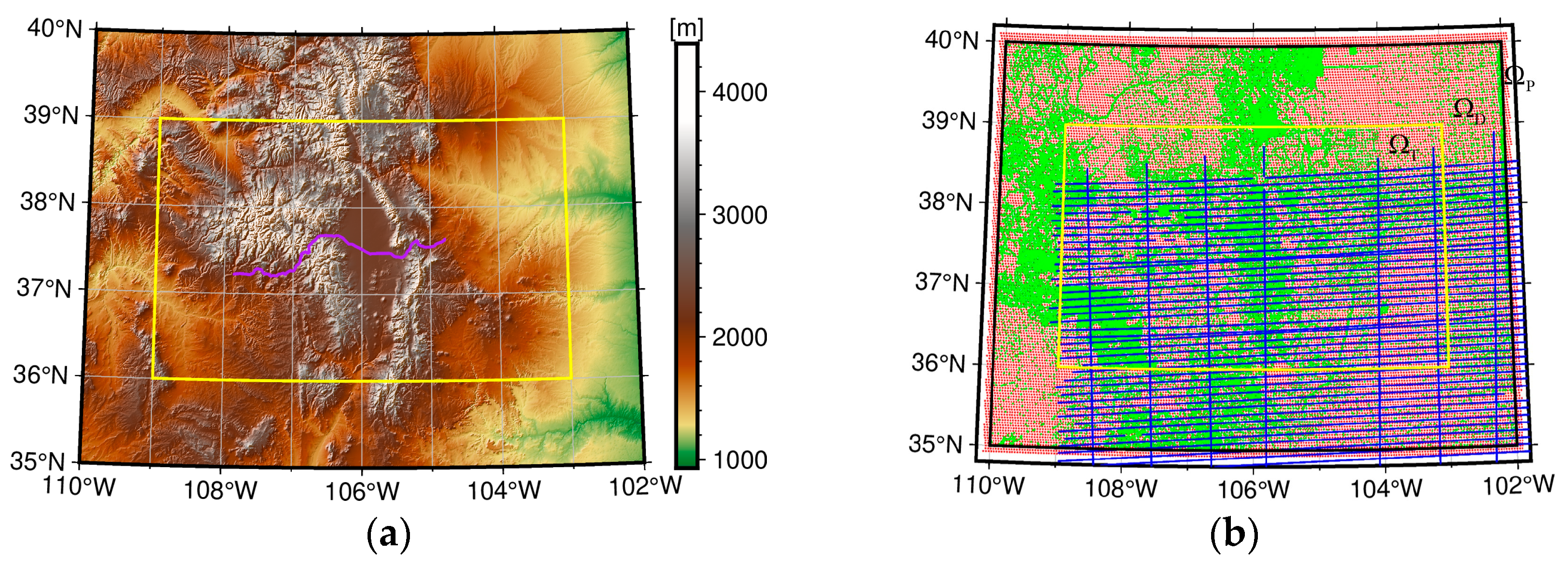
3. Data and Study Area

The study area is located in the state of Colorado, USA. It is approximately 550 km by 730 km, with longitude varying from ${110}^{\circ }\mathrm{W}$ to ${102}^{\circ }\mathrm{W}$ and latitude varying from ${35}^{\circ }\mathrm{N}$ to ${40}^{\circ }\mathrm{N}$ (Figure 1a). This study area is considered to be representative due to the rough topography and high elevation. Meanwhile, we have access to the gravity datasets for the area. In addition, fourteen contributing groups of the Colorado1-cm geoid experiment have calculated gravity field models for this area, which helps in the interpretation of the results.

3.1. Terrestrial and Airborne Gravity Data

There were 59,303 terrestrial gravity observations provided by the National Geospatial Intelligence Agency and National Geodetic Survey (NGS). Figure 1b shows that the terrestrial gravity observations were unevenly distributed over the entire study area. They were sparse in the eastern parts, but dense in the central and western parts. Saleh et al. [62] estimate that the root-mean-square (RMS) error of NGS’s terrestrial gravity data is about 2.2 mGal.

The GRAV-D (Gravity for the Redefinition of the American Vertical Datum) Science Team provided a total of 283,716 airborne gravity observations (from MS05 block). The observations were distributed across 56 distinct flight lines, and the average flight altitude was approximately 6200 m. The flight lines covered only the southwestern part of the study area. For the airborne gravity data, the along-track spacing was approximately 100 m, while that between the cross-tracks was approximately 10 km. The GRAV-D Science Team suggests applying a frequency domain low-pass filter to the data to remove excess short-wavelength noise [63]. Many studies have exhibited that the RMS error of the GRAV-D airborne gravity data is approximately 2 mGal [63,64,65].

3.2. Data Preprocessing

After error detection and outlier removal, a total of 58,123 terrestrial gravity observations were retained. Therefore, the average point distance was approximately 2.7 km for the terrestrial dataset. For the terrestrial data, Helmert orthometric heights H were provided. Thus, surface gravity anomalies were obtained on Earth’s surface in [45] (p. 204):

$$\mathsf{\Delta }g=g-{\gamma }_0\left[1-2\left(1+f+m-2f{\sin }^2\phi \right)\frac{H^{\ast }}{a}+3{\left(\frac{H^{\ast }}{a}\right)}^2\right],$$

(17)

where g is the measured gravity and ${\gamma }_0$ is the normal gravity at the surface of the reference ellipsoid, computed using Somigliana’s formula [45]. f and a are the geometrical fattening and semi-major axes of the reference ellipsoid GRS80, respectively. m is the ratio of centrifugal and gravity acceleration at its equator, $\phi$ is the geodetic latitude, and H^* is the normal height. To transform the orthometric heights H provided by terrestrial gravity points to the required normal heights H^*, the correction term synthesized from the EGM2008 quasigeoid to geoid separation model was used [66].

For the airborne gravity data, a Gaussian low-pass filter [67] was used to remove excess short-wavelength noise. To reduce the computational burden, we sampled the data at a frequency of 1/8 Hz. The basis for reducing the sampling frequency was that there were strong correlations between consecutive observations after Gaussian low-pass filtering. After down-sampling, the number of airborne gravity observations was 35,465, with an average point distance of approximately 1 km along the track. The sampling interval was selected because it provided a reasonable point density for the required spatial resolution (computing a $1^{\prime }\times 1^{\prime }$ quasigeoid model) in this study (see [67,68] for more details). Because certain observations were found to lie outside of the study area (see Figure 1b), we excluded these observations, resulting in a total of 32,033 retained airborne gravity observations. We transformed the airborne gravity data from the measured absolute gravity g to gravity disturbance $\delta g$ using the following equation:

$$\delta g=g-\gamma ,$$

(18)

wherein $\gamma$ denotes the normal gravity of the observation point.

The atmospheric correction $\delta g_{\mathrm{ATM}}$ was calculated according to [69]:

$$\delta g_{\mathrm{ATM}}=0.874-9.9\times 10^{-5}H+3.5625\times 10^{-9}{H}^2.$$

(19)

The atmospheric correction values were added to g of all gravity points in the terrestrial and airborne datasets [70].

4. Experiment Settings

4.1. Remove–Compute–Restore Technique

In this study, the SRBFs model represents the residual disturbing potential, which is the full disturbing potential minus the GGM disturbing potential and the topographic disturbing potential. The GGM provides the long-wavelength parts of the regional gravity field, while the topographic model provides the topographic effects and smooths the input gravity measurements. SRBFs can extend the regional gravity field to very short spatial scales using dense gravity data. These procedures are implemented within the framework of the remove–compute–restore (RCR) technique [71]. Using the RCR technique, the GGM and topographic gravity model (TGM) components were removed from the gravity anomaly (terrestrial gravity dataset) and gravity disturbance (airborne gravity dataset) as follows:

$$\mathsf{\Delta }{g}_{\mathrm{res}}=\mathsf{\Delta }g-\mathsf{\Delta }{g}_{\mathrm{R}},$$

(20)

$$\delta g_{\mathrm{res}}=\delta g-\delta g_{\mathrm{R}}.$$

(21)

Then, the SRBFs were used to process the residual measurements ($\mathsf{\Delta }{g}_{\mathrm{res}}$ and $\delta g_{\mathrm{res}}$) in order to calculate the residual disturbing potential ${\widehat{T}}_{\mathrm{res}}$. Finally, the removed components $T_{\mathrm{R}}$ were restored:

$$\widehat{T}={\widehat{T}}_{\mathrm{res}}+T_{\mathrm{R}}.$$

(22)

In this study, we employed the setup described by [72]: the GGM XGM2016 [73] up to a maximum degree of 719 was removed from the terrestrial and airborne data; furthermore, we removed the TGM dV_ELL_Earth2014 [74] from degree 720 to degree 2160 and the residual terrain model ERTM2160 [75] from the terrestrial data; as well as removing the dV_ELL_Earth2014 from degree 720 to degree 5480 from the airborne data. This is because the above two TGMs were both calculated using the SRTM v4.1 topography model [76], and had similar gravity signals at the same SH degree.

Table 1. The statistics of the (residual) gravity anomaly observations and the (residual) gravity disturbance observations (unit: mGal).

Observations	Min	Max	Mean	STD
Terrestrial $\mathsf{\Delta }g$	−141.50	212.45	5.92	38.15
Terrestrial $\mathsf{\Delta }{g}_{\mathrm{res}}$	−136.09	75.31	0.83	6.92
Airborne $\delta g$	−44.64	118.91	6.10	28.81
Airborne $\delta g_{\mathrm{res}}$	−18.88	21.38	0.37	3.23

indicates that after removing the GGM and TGMs components, the standard deviations (STDs) of the terrestrial and airborne observations decreased by 81.9% and 88.8%, respectively. Figure 2 exhibits the magnitudes of the (residual) gravity anomaly and (residual) gravity disturbance observations.

4.2. Maximum Degree of Expansion

According to [72,77], the maximum expansion degree $l_{\max }$ of the SRBFs is correlated with the mean point distance of the heterogeneous observation sr, namely,

$$l_{\max }\le \frac{\pi R}{\mathrm{sr}}.$$

(23)

Based on Section 3.2, with $\mathrm{sr}\approx 3.0 \mathrm{km}$, the maximum degree $l_{\max }\approx 6700$. Nevertheless, this is only a recommended value, and the resulting model may be sub-optimal. We adapted this recommended value to determine $l_{\max }$ based on the control data, and the specific method was a three-step procedure: (1) the candidate values of $l_{\max }$ were determined according to its recommended value; (2) for each candidate value of $l_{\max }$, the optimal regularization parameters of LASSO and Tikhonov regularization were selected using AIC, respectively, and the RMS errors of the solutions were calculated based on the control data; (3) the minimum RMS error was found, and the corresponding $l_{\max }$ was the optimal selection. The numerical results indicate that $l_{\max }$ should be set to 5500 (see Section 5.1).

4.3. Types of the SRBFs

Based on previous studies [77,78], different types of SRBFs can be employed in the analysis step (unknown parameter estimation) and the synthesis step (calculating the gravitational functions), respectively. According to [72], we employed the Shannon function and the cubic polynomial (CuP) function.

Table 2. Legendre coefficients of the SRBFs.

Function Types	Legendre Coefficients
Shannon function	${\psi }_l=\{\begin{array}{ll}1,\hfill & \mathrm{for} l\in [0,l_{ma\mathit{x}}]\hfill \\ 0,\hfill & \mathrm{else}\hfill \end{array}$
CuP function	${\psi }_l=\{\begin{array}{cc}{(1-\frac{l}{l_{\max }})}^2(1+\frac{2l}{l_{\max }}),& \mathrm{for} l\in [0,l_{\max }]\hfill \\ 0,& \mathrm{else}\hfill \end{array}$

lists the corresponding Legendre coefficients.

The Shannon function did not smooth the gravity signal in the corresponding spectral band. Conversely, the CuP function smoothed the gravity signal from the beginning in the spectral domain. In this study, we used the Shannon function in the analysis step and the CuP function in the synthesis step (see [72] for detailed reasons). This differs from the setup of [72] in that they used the Shannon and CuP functions for the terrestrial and airborne gravity data, respectively, in the analysis step.

4.4. Defining the Target, Data, and Parameterization Area

To avoid the edge effects caused by the spatial truncation of data and basis functions as much as possible, the necessary setting for the target area ${\mathsf{\Omega }}_{\mathrm{T}}$, data area ${\mathsf{\Omega }}_{\mathrm{D}}$, and parameterization area ${\mathsf{\Omega }}_{\mathrm{P}}$ was ${\mathsf{\Omega }}_{\mathrm{T}}\subset {\mathsf{\Omega }}_{\mathrm{D}}\subset {\mathsf{\Omega }}_{\mathrm{P}}$. ${\mathsf{\Omega }}_{\mathrm{T}}$ and ${\mathsf{\Omega }}_{\mathrm{D}}$ are given in Section 3, respectively. Thus, only the margin ${\eta }_{\mathrm{P},\mathrm{D}}$ needs to be defined. Naeimi [15] and Lieb et al. [77] both defined the width of ${\eta }_{\mathrm{P},\mathrm{D}}$ through an experiential formula, and the latter was approximately twice the width of the former. To minimize the edge effects, we followed the latter. Liu et al. [72] gave the final equation:

$${\eta }_{\mathrm{P},\mathrm{D}}=\frac{{360}^{\circ }}{l_{\max }\times \cos ({\left|\phi \right|}_{\max })},$$

(24)

where ${\left|\phi \right|}_{\max }$ denotes the maximum absolute value of the latitude of ${\mathsf{\Omega }}_{\mathrm{T}}$, and thus the width of the margin ${\eta }_{\mathrm{P},\mathrm{D}}\approx 0.1^{\circ }$ (see Figure 1b).

4.5. Locations of the SRBFs

The grid type controls the SRBF locations. Several grid types have been studied in the literature [6,7]. In this study, the commonly used Reuter grid [79] was employed. Given $l_{\max }$, the number of the Reuter grid points on the global scale can be approximated by the following equation [16,80]:

$$I\le 2+\frac{4}{\pi }{(l_{\max }+1)}^2.$$

(25)

As already mentioned in Section 4.2, $l_{\max }$ was selected as 5500. Thus, the total number of Reuter grid points in ${\mathsf{\Omega }}_{\mathrm{P}}$ was N = 31,595 (see Figure 1b).

4.6. Weight Matrix of Observations

The weight matrices for both terrestrial observations (${\mathit{P}}_1$) and airborne observations (${\mathit{P}}_2$) were set as the unit matrix because we assumed that the observations have no correlations and have the same accuracy for one data type. This assumption is commonly used [22,81]. In the data descriptions in Section 3.1, the priori noise STDs of terrestrial and air-borne data are provided. The terrestrial and airborne data contained errors with STDs of ~2.2 mGal and ~2.0 mGal, respectively. Therefore, we were able to obtain the scale factors ${\widehat{\sigma }}_1^2=4.84\times {10}^{-10}{\mathrm{m}}^2/{\mathrm{s}}^4$ and ${\widehat{\sigma }}_2^2=4.00\times {10}^{-10}{\mathrm{m}}^2/{\mathrm{s}}^4$. Thus, the weight matrix of the measurements can be estimated by

$$\mathit{P}=\left[\begin{array}{cc}\frac{1}{{\widehat{\sigma }}_1^2}{\mathit{P}}_1& \mathbf{0}\\ \mathbf{0}& \frac{1}{{\widehat{\sigma }}_2^2}{\mathit{P}}_2\end{array}\right].$$

(26)

4.7. Computation of the Disturbing Potential Functionals

By solving Equation (9) or Equation (13), the residual disturbing potential ${\widehat{T}}_{\mathrm{res}}$ was synthesized by

$${\widehat{\mathit{T}}}_{\mathrm{res}}\left(\mathit{x}\right)=\mathit{B}\left(\mathit{x}\right)\widehat{\mathit{\beta }}$$

(27)

Then, Equation (22) was used to calculate the disturbing potential $\widehat{T}$. For the computation of the disturbing potential functionals, we followed the basic agreements for the computation of the Colorado 1 cm geoid experiment [82].

5. Results

In the target area, two datasets were available as control data. The first was the geometric geoid heights of the 222 Geoid Slope Validation Survey 2017 (GSVS17), which were provided by the NGS (see Figure 1a). The accuracy of the GSVS17 GPS/leveling dataset was approximately 1.2 cm [43]. The other was a (quasi) geoid grid model with $1^{\prime }\times 1^{\prime }$ resolution, which corresponded to the target area. The weighted least-squares solution of the Tikhonov regularization was included to verify the quality of the LASSO solution. Comparisons of the solutions of the two methods are provided.

5.1. The Estimated Parameters

We took the GSVS17 GPS/leveling dataset as the control dataset and used the three-step procedure in Section 4.2 to obtain the optimal $l_{\max }$.

Table 3. Evaluations of the different geoid models based on various $l_{\max }$ values.

	LASSO		Tikhonov Regularization
${\mathit{l}}_{\mathbf{max}}$	$\mathit{\lambda }$	RMS (cm)	$\mathit{\mu }$	RMS (cm)
5000	$1.0\times {10}^7$	2.93	$6.14\times {10}^{12}$	2.89
5500	$1.1\times {10}^7$	2.82	$6.20\times {10}^{12}$	2.79
6000	$1.1\times {10}^7$	2.91	$6.30\times {10}^{12}$	2.88
6500	$1.2\times {10}^7$	3.07	$6.46\times {10}^{12}$	3.05
6700	$1.2\times {10}^7$	3.16	$6.54\times {10}^{12}$	3.14

shows the optimal regularization parameters corresponding to different $l_{\max }$ values, as well as the RMS errors of the solutions. The results demonstrate that the RMS value of the LASSO solution and the Tikhonov regularization solution were both at their smallest when $l_{\max }$ was approximately 5500, with respect to the control data. Consequently, the maximum expansion degree $l_{\max }$ of the SRBFs was set to 5500. Figure 3 exhibits the residuals of parameter models with respect to the input data when $l_{\max }=5500$. For the LASSO solution, the residuals of the terrestrial data had a mean value of −0.46 mGal and an STD of 2.43 mGal, and the residuals of the airborne data had a mean value of −0.25 mGal and a STD of 1.60 mGal; for the Tikhonov regularization solution, the residuals of the terrestrial data had a mean value of −0.41 mGal and a STD of 2.38 mGal, and the residuals of the airborne data have a mean value of −0.23 mGal and a STD of 1.57 mGal. Considering the priori noise STDs of the input data, Figure 3 indicates that the selected parameter models fit the input data well.

Figure 4 displays the histograms of the parameters estimated by LASSO and Tikhonov regularization. It can be seen that the LASSO solution follows the Laplacian distribution, whereas the Tikhonov regularization solution follows the Gaussian distribution. As mentioned earlier, the LASSO can completely shrink some of the parameters to zero. For the LASSO, there were 7859 non-zero parameters among 31,595 estimated parameters. In other words, approximately 75.1% of the parameters were shrunk to zero. The sparse nature of the LASSO considerably reduced the final number of the SRBFs, making the model smaller and simpler.

Figure 5 shows the estimated parameters $\widehat{\mathit{\beta }}$ and their STDs. Figure 5a,c reveal that most of the parameters near zero in the Tikhonov regularization solution shrunk to zero in the LASSO solution. However, the distribution of the remaining parameters was almost identical between the two solutions. Note that Figure 2b,d and Figure 5a,c exhibit obvious correlations. Most non-zero parameters are located close to observation points, and more SRBFs are removed by LASSO in areas with sparser data. At the same time, the estimated parameters near the points with larger residual gravity anomalies and residual gravity disturbances are larger. These indicate that the distribution of the non-zero parameters was adapted to the gravity data distribution and signal variation, and the LASSO removed redundant parameters based on the data-driven model selection criterion AIC. Figure 5b,d display the STDs of the parameters estimated by the LASSO and Tikhonov regularization, which are similar in that larger STDs occurred at data gaps and the margin between ${\mathsf{\Omega }}_{\mathrm{D}}$ and ${\mathsf{\Omega }}_{\mathrm{P}}$ (see Figure 1b and Figure 2).

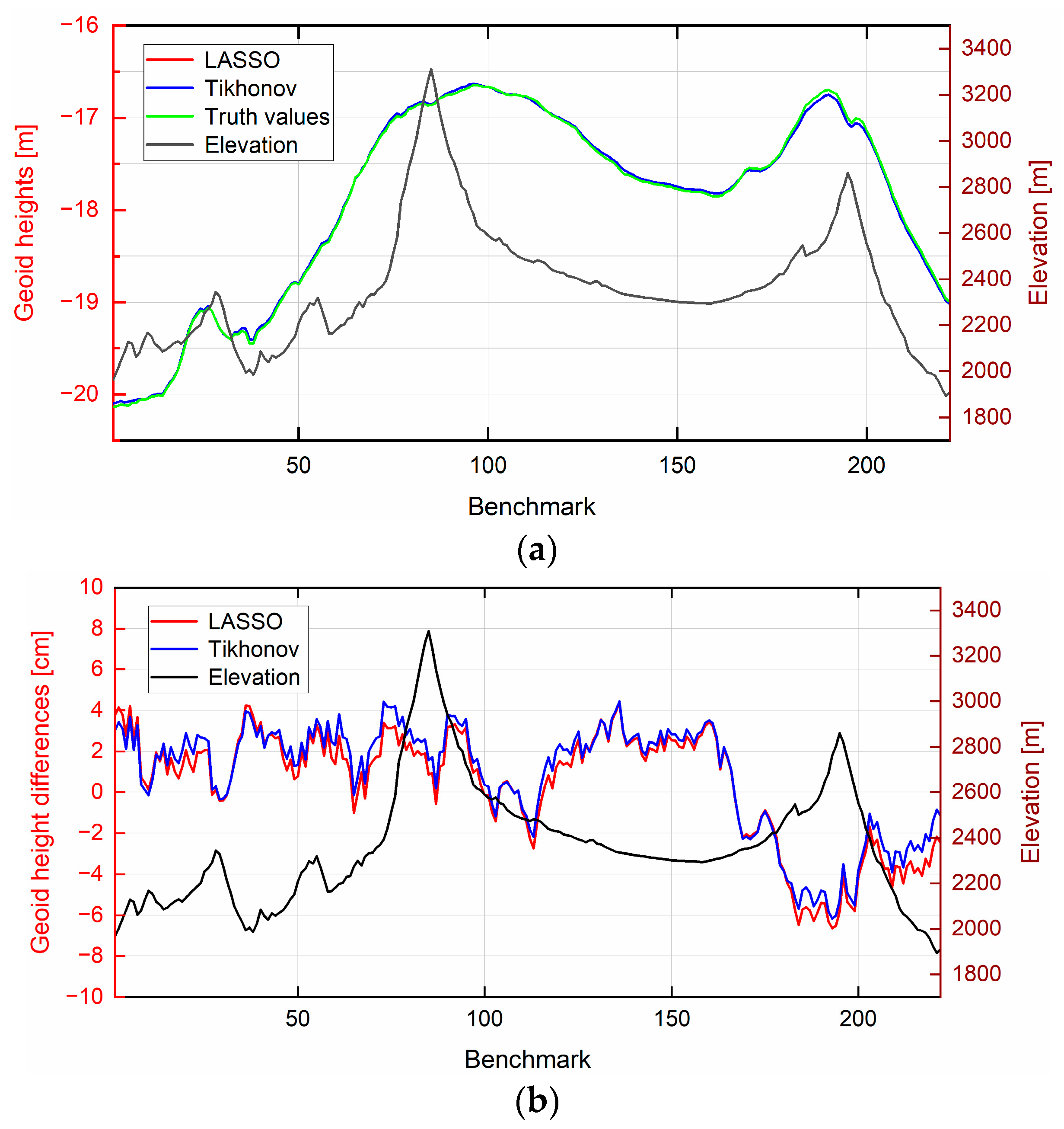
5.2. GPS/Leveling Comparisons

We evaluated gravimetric geoid heights using the GSVS17 GPS/leveling control datasets.

Table 4. Statistics of differences between geometric and gravimetric geoid heights at the benchmarks (unit: cm).

Solution	Min	Max	Mean	RMS	STD
LASSO	−6.63	4.38	0.37	2.82	2.79
Tikhonov	−6.16	4.44	0.76	2.79	2.75

presents the statistics of the differences between geometric and gravimetric geoid heights. For the GSVS17 benchmarks, the RMS errors were calculated to be 2.82 cm and 2.79 cm using the LASSO and Tikhonov regularization methods, respectively. Figure 6 illustrates the geometric and gravimetric geoid heights and their differences at the GSVS17 benchmarks. Figure 6a indicates good agreements between the computed gravimetric geoid heights and the geometric geoid heights (truth values). Figure 6b demonstrates that both LASSO and Tikhonov regularization solutions exhibit similar trends regarding the differences in geoid heights. Specifically, between marks 1 and 181, the difference curves of the two methods are very close. However, in this interval, more points in the LASSO solution had differences closer to zero than the Tikhonov regularization solution. Conversely, between marks 182 and 222, the performance of the Tikhonov regularization solution is slightly better than that of the LASSO solution. To summarize, the LASSO and Tikhonov regularization solutions performed similarly in GPS/leveling comparisons, but the latter outperformed the former slightly.

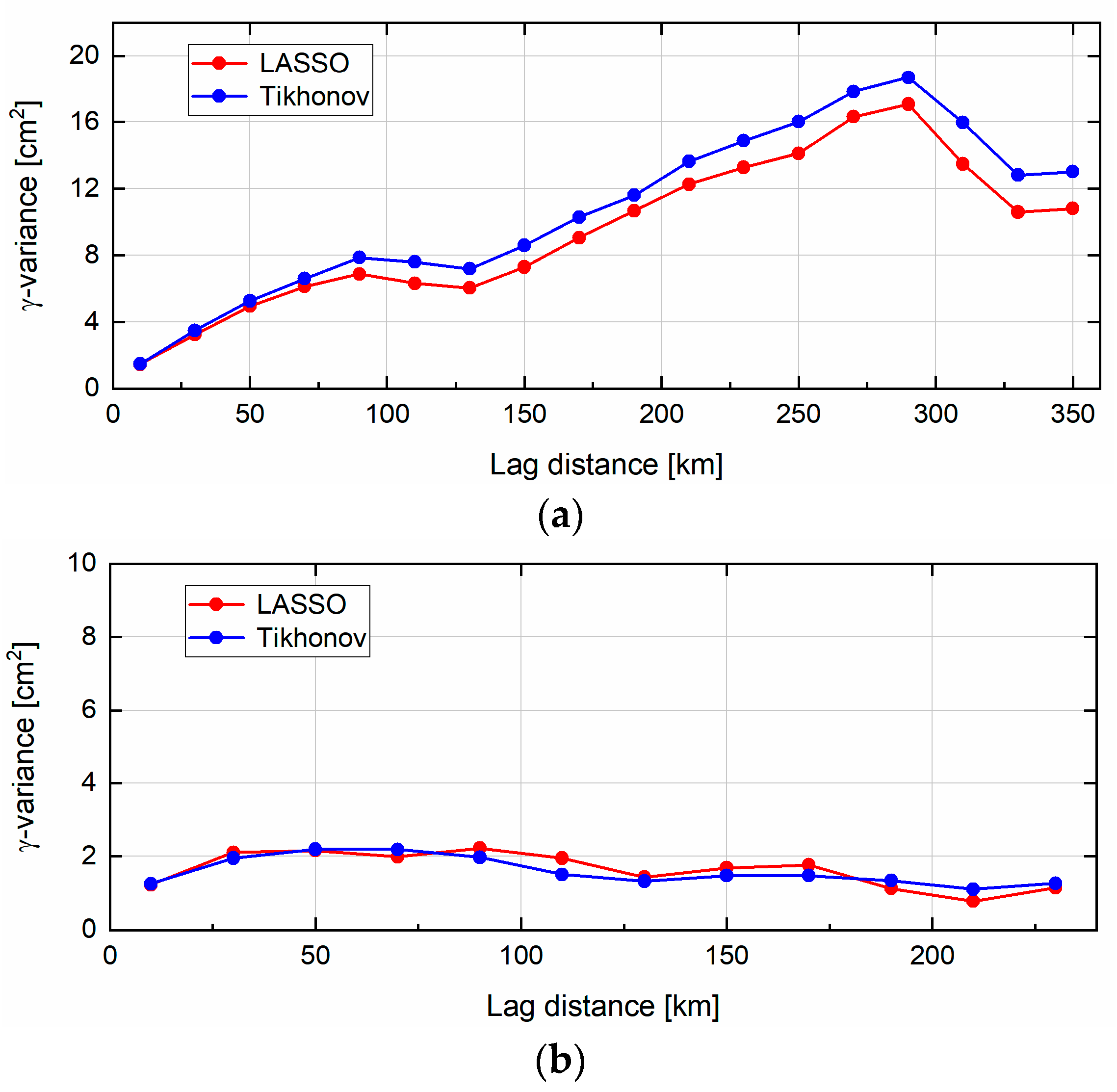
5.3. Variogram Analysis of the Differences

Information about the quality of the LASSO and Tikhonov regularization solutions as spatial scale functions is provided by variogram analyses of the differences between geometric and gravimetric geoid heights at the GPS/leveling control datasets [81]. Figure 7 presents the empirical variograms of the LASSO and Tikhonov regularization solutions. A variogram expresses the variance of the observed differences between the geometric and gravimetric geoid heights for point pairs as a function of lag distances. According to [83], the term “gammavariance” denotes the variance of the differences at a given lag distance.

In Figure 7a, for the GSVS17 benchmarks, the gammavariances of the LASSO and Tikhonov regularization solutions are shown to increase rapidly when lag distances are less than 290 km and range between ~1.5 cm² and ~17.8 cm²; they decrease rapidly to ~11.7 cm² when the lag distances are smaller than 330 km and increase again until the lag distance is 350 km. Wang et al. [43] analyzed that the significant differences after mark 160 (see Figure 6b) are the primary reason for the large gammavariance values in Figure 7a. The empirical variograms at GSVS17 between marks 1 and 160 are shown in Figure 7b, which demonstrates no large fluctuations in the gammavariance values. By comparing the empirical variograms between the LASSO and Tikhonov regularization solutions, it can be observed that the former was slightly larger than the latter when the lag distances were between 0 and 50 km and between 80 and 180 km. On the other hand, the former had slightly lower gammavariances when the lag distances were between 50 and 70 km and between 180 and 240 km. In short, the variogram analysis of the differences indicates that the performances of the LASSO and the Tikhonov regularization solution are very close, but the latter is slightly superior.

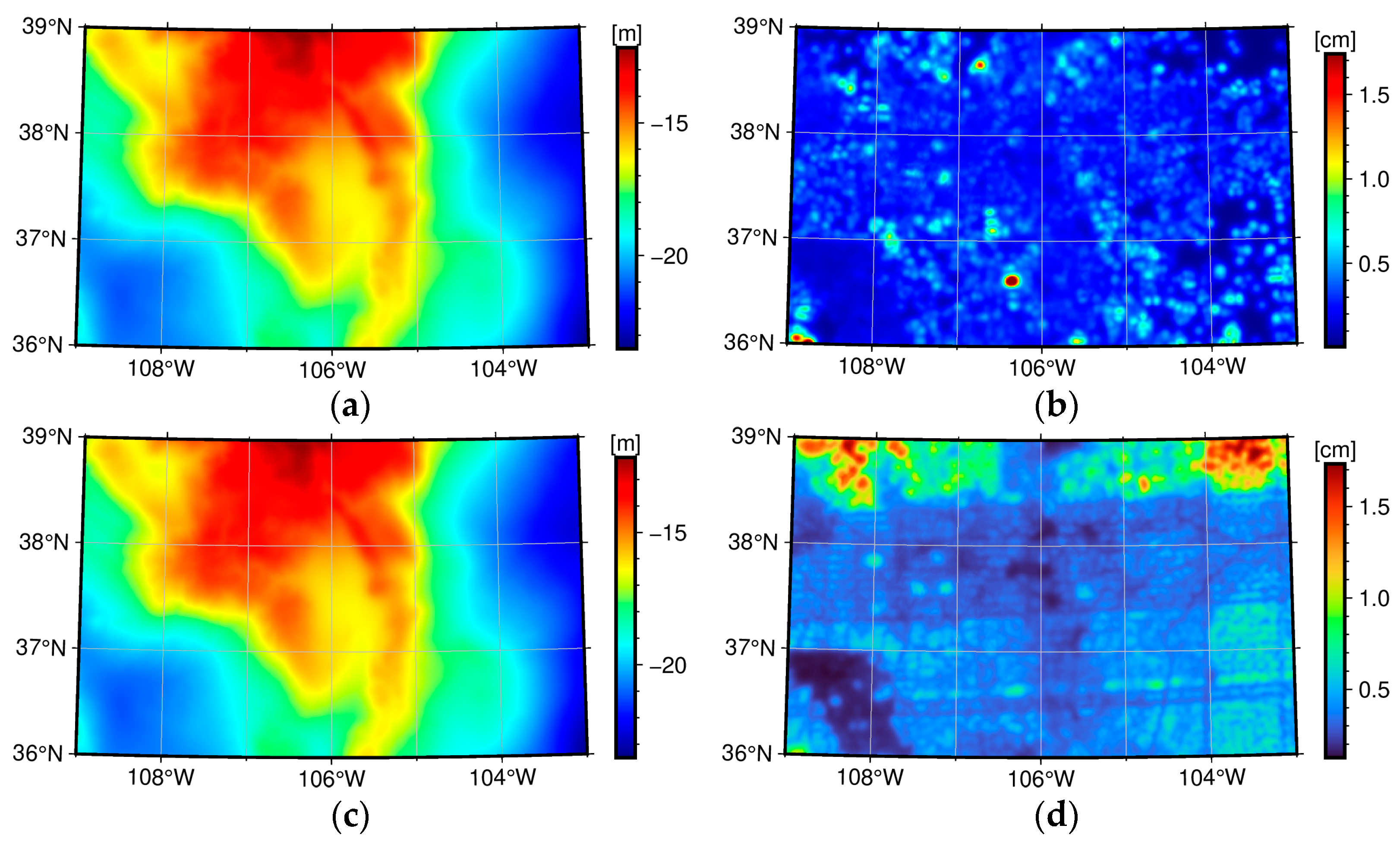
5.4. Area Comparison of Quasigeoid Model (Grids of $1^{\prime }\times 1^{\prime }$)

The quasigeoid models are given on a $1^{\prime }\times 1^{\prime }$ grid over the target area between longitude ${109}^{\circ }\mathrm{W}$ to ${103}^{\circ }\mathrm{W}$ and latitude ${36}^{\circ }\mathrm{N}$ to ${39}^{\circ }\mathrm{N}$ (see Figure 8). For the target area, the truth value of the quasigeoid model is unknown. However, fourteen contributing groups of the 1 cm geoid experiment in Colorado have used different methods to calculate gravity field models for this area. Therefore, the quasigeoid models of the LASSO and Tikhonov regularization solution were compared with the mean of all groups. Figure 9 illustrates the comparison results. According to the comparison results, the differences between the LASSO solution and group mean ranged between −5.78 and 9.67 cm, with a mean value of 0.90 cm, a STD value of 1.63 cm, and an RMS value of 1.86 cm; for the Tikhonov regularization solution, the differences from the group mean ranged between −8.11 and 9.32 cm, with a mean value of 0.97 cm, a STD value of 1.64 cm, and an RMS value of 1.91 cm. Since the RMS values of the fourteen individual solutions of the 1 cm geoid experiment to the group mean ranged between 1.6 and 5.3 cm [43], the LASSO and Tikhonov regularization solutions in this study provided good results, and their model precisions were comparable. Figure 9c illustrates the quasigeoid model differences between the LASSO and Tikhonov regularization solution; the differences varied between −3.58 and 7.63 cm, with a mean value of −0.08 cm. The comparison results reveal that the quasigeoid models of the LASSO and Tikhonov regularization solutions were in good agreement, besides the northern and southeastern parts of the target region, and this was related to the scarcity of observations within the northern and southeastern parts (see Figure 1b and Figure 2).

Through error propagation, the approximate covariance matrix was used to calculate the formal noise covariance matrix of the height anomalies derived by the LASSO solution. The STD maps of the modeled height anomalies are shown in Figure 8b,d. Unlike the quasigeoid models, the STD maps of the height anomalies modeled by LASSO and Tikhonov regularization were remarkably different. For Tikhonov regularization, the formal noise STDs ranged from a few millimeters to 1.73 cm, and the STDs were larger in the region with sparser observations. For LASSO, although the largest STD reached 2.56 cm, its STD map was unexpected. For example, the STDs of the height anomalies in the regions with sparser observations were considerably small, such as some regions in the eastern and northern parts of the target area.

Fan and Li [35] provided an iterative method to solve the LASSO and calculate the covariance matrix of the sparse SRBF parameters, and they also ignored the uncertainty of the zero parameters, which is the same as the covariance matrix we provide in Section 2.4. We attempted to solve LASSO by Fan’s method and calculate the STDs of height anomalies. In terms of the distribution of non-zero SRBF parameters and the precision of the quasigeoid model, Fan’s method was almost identical to the method adopted in this work. Figure 10 illustrates the STD map of height anomalies calculated using Fan’s method. Similarly, the STDs of the height anomalies calculated by Fan’s method were smaller in the region with sparser observations than in the region with denser observations. A major reason is that there were fairly few non-zero SRBF parameters in the region with sparser observations; thus, the contribution of these SRBFs to height anomalies in the corresponding regions was quite limited when the errors were propagated. For Fan’s method, there was another problem that all STDs were numerically smaller than our proposed method. This is because Fan’s method uses the corresponding sandwich formula to calculate the covariance matrix of the sparse SRBF parameters. Thus, for the STDs of the modeled height anomalies, the method we propose in this work is more conservative, but its calculation is also less realistic. In this target area, the results of the 1 cm geoid experiment in Colorado indicate that the best calculation precision of the quasigeoid model is approximately 2 cm [43]. Therefore, the STDs of the Tikhonov regularization solution are more realistic than our proposed method and Fan’s method.

6. Discussion

To verify the effectiveness of the LASSO, the LASSO solution was compared with the weighted least-squares solution based on Tikhonov regularization. To determine the maximum expansion degree of the SRBFs and Reuter grid parameter, a three-step procedure was used. The numerical results indicated that when $l_{\max }$ is 5500, the fitted results of the LASSO and weighted least-squares solutions are the best. The parameter estimation results exhibited that the LASSO can obtain a very sparse model. Most parameters with values close to zero in the Tikhonov regularization solution shrunk to zero in the LASSO solution, whereas the remaining parameters had nearly the same distribution. Although the number of zero parameters accounted for 75.1% of all parameters, the sparse model represented the gravity structure well.

We calculated the geoid heights at the GSVS17 benchmarks, as well as the quasigeoid models (grids of $1^{\prime }\times 1^{\prime }$) of the target area. Comparisons with the GPS/leveling control dataset exhibited that for the GSVS17 benchmarks, the LASSO solution was slightly worse than the Tikhonov regularization solution (the RMS of the differences increases from 2.79 to 2.82 cm). At the GSVS17 benchmarks, the empirical variance maps implied an improvement in the gammavariances for the LASSO solution compared to those of the Tikhonov regularization solution when the lag distances were between 50 and 70 km and between 180 and 240 km; however, the situation was the opposite when the lag distances were between 0 and 50 km and between 80 and 180 km. For the quasigeoid models covering the target area, the LASSO solution was closer to the group mean than the Tikhonov regularization solution (the RMS of the differences improves from 1.91 to 1.86 cm). In addition, the quasigeoid model differences between the LASSO and the Tikhonov regularized solution ranged between −3.58 and 7.63 cm, with a mean value of −0.08 cm. Using the approximate covariance matrix derived in this study, the formal noise STDs of the LASSO-derived height anomalies were calculated by error propagation, but the results were unrealistic. We also tried a method in the statistics field, but the same problem emerged. In contrast, the STDs of the Tikhonov regularization solution are more realistic.

Referring to the results of the Colorado 1 cm geoid experiment [43], the LASSO and Tikhonov regularization solutions provided good results in terms of model accuracy, even if the study area consisted of rugged mountains with considerable data gaps. However, the sparse SRBFs method has two limitations: first, when combining multiple gravity datasets, an additional procedure is required in order to estimate their variance factors or relative weights; second, the noise covariance matrix of the derived model cannot be calculated realistically at the present stage. The determination of the weights of heterogeneous data contributes to their optimal combination, while the covariance estimation of the L1-norm regularized solution is crucial for the realization of globally uniform height systems. Solving the above two problems is one of our future research goals. Considering the urgent need for 1 cm geoid models, providing validation data with sub-centimeter accuracy is also crucial for further research.

7. Conclusions

In this study, the SRBFs method based on sparse regularization was used to compute the (quasi) geoid model in Colorado, USA. To reduce the complexity of the model and because the system was singular and/or ill-posed, L1-norm regularization (LASSO) was introduced. LASSO can not only regularize the system, but also produce a sparse solution. According to the data-driven model selection criterion AIC, LASSO is able to automatically select the model parameters, i.e., shrinking some of the parameters to zero, thereby simplifying the model. Moreover, it has high computational efficiency. To the best of our knowledge, it is the first study to apply the LASSO to SRBFs-based modeling of the regional gravity field in real gravity observation data. The experimental results demonstrate that the LASSO solution does not significantly degrade the performance of the model compared to the Tikhonov regularization solution. Therefore, LASSO proves to be competitive. This method automatically selects the SRBFs based on signal variation and gravity data distribution, considerably reducing the number of SRBFs and satisfying the precision required for modeling. The sparse SRBFs method is a promising alternative approach to large-scale and high-resolution gravity field modeling tasks.

References

1. Torge, W. Geodesy; Walter de Gruyter: Berlin, Germany, 2001. [Google Scholar]
2. Vaníček, P.; Krakiwsky, E.J. Geodesy; Elsevier Science Publishers: New York, NY, USA, 1987. [Google Scholar]
3. Hofmann-Wellenhof, B.; Moritz, H. Physical Geodesy; Springer: Wien, Austria, 2006. [Google Scholar]
4. Li, X.P. Using radial basis functions in airborne gravimetry for local geoid improvement. J. Geod. 2018, 92, 471–485. [Google Scholar] [CrossRef]
5. Simons, F.J.; Dahlen, F.A.; Wieczorek, M.A. Spatiospectral concentration on a sphere. SIAM Rev. 2006, 48, 504–536. [Google Scholar] [CrossRef]
6. Eicker, A. Gravity Field Refinement by Radial Basis Functions from In-Situ Satellite Data. Ph.D. Thesis, Bonn University, Bonn, Germany, 2008. [Google Scholar]
7. Wittwer. Regional Gravity Field Modelling with Radial Basis Functions. Ph.D. Thesis, Delft University of Technology, Delft, The Nederland, 2009. [Google Scholar]
8. Bucha, B.; Bezdek, A.; Sebera, J.; Janak, J. Global and Regional Gravity Field Determination from GOCE Kinematic Orbit by Means of Spherical Radial Basis Functions. Surv. Geophys. 2015, 36, 773–801. [Google Scholar] [CrossRef]
9. Schmidt, M.; Fengler, M.; Mayer-Gurr, T.; Eicker, A.; Kusche, J.; Sanchez, L.; Han, S.C. Regional gravity modeling in terms of spherical base functions. J. Geod. 2007, 81, 17–38. [Google Scholar] [CrossRef]
10. Klees, R.; Liu, X.; Wittwer, T.; Gunter, B.C.; Revtova, E.A.; Tenzer, R.; Ditmar, P.; Winsemius, H.C.; Savenije, H.H.G. A Comparison of Global and Regional GRACE Models for Land Hydrology. Surv. Geophys. 2008, 29, 335–359. [Google Scholar] [CrossRef]
11. Klees, R.; Tenzer, R.; Prutkin, I.; Wittwer, T. A data-driven approach to local gravity field modelling using spherical radial basis functions. J. Geod. 2008, 82, 457–471. [Google Scholar] [CrossRef]
12. Tenzer, R.; Klees, R. The choice of the spherical radial basis functions in local gravity field modeling. Stud. Geophys. Geod. 2008, 52, 287–304. [Google Scholar] [CrossRef]
13. Panet, I.; Kuroishi, Y.; Holschneider, M. Wavelet modelling of the gravity field by domain decomposition methods: An example over Japan. Geophys. J. Int. 2011, 184, 203–219. [Google Scholar] [CrossRef]
14. Bentel, K.; Schmidt, M.; Gerlach, C. Different radial basis functions and their applicability for regional gravity field representation on the sphere. GEM-Int. J. Geomath. 2013, 4, 67–96. [Google Scholar] [CrossRef]
15. Naeimi, M. Inversion of Satellite Gravity Data Using Spherical Radial Base Functions. Ph.D. Thesis, Leibniz Universität Hannover, Hanover, Germany, 2013. [Google Scholar]
16. Naeimi, M.; Flury, J.; Brieden, P. On the regularization of regional gravity field solutions in spherical radial base functions. Geophys. J. Int. 2015, 202, 1041–1053. [Google Scholar] [CrossRef]
17. Foroughi, I.; Safari, A.; Novák, P.; Santos, M.C. Application of radial basis functions for height datum unification. Geosciences 2018, 8, 369. [Google Scholar] [CrossRef]
18. Wu, Y.H.; Luo, Z.C.; Zhong, B.; Xu, C. A multilayer approach and its application to model a local gravimetric quasi-geoid model over the North Sea: QGNSea V1.0. Geosci. Model Dev. 2018, 11, 4797–4815. [Google Scholar] [CrossRef]
19. Klees, R.; Slobbe, D.C.; Farahani, H.H. How to deal with the high condition number of the noise covariance matrix of gravity field functionals synthesised from a satellite-only global gravity field model? J. Geod. 2019, 93, 29–44. [Google Scholar] [CrossRef] [PubMed]
20. Lin, M. Regional Gravity Field Recovery Using the Point Mass Method. Ph.D. Thesis, University of Hannover, Hanover, Germany, 2015. [Google Scholar]
21. Lieb, V. Enhanced Regional Gravity Field Modeling from the Combination of Real Data via MRR. Ph.D. Thesis, Technischen Universität München, Munich, Germany, 2017. [Google Scholar]
22. Wu, Y. Regional Gravity Field Modeling from Heterogeneous Data Sets by Using Poisson Wavelets Radial Basis Functions. Ph.D. Thesis, Wuhan University, Wuhan, China, 2016. [Google Scholar]
23. Bentel, K.; Schmidt, M.; Rolstad Denby, C. Artifacts in regional gravity representations with spherical radial basis functions. J. Geod. Sci. 2013, 3, 173–187. [Google Scholar] [CrossRef]
24. Lin, M.; Denker, H.; Muller, J. A comparison of fixed- and free-positioned point mass methods for regional gravity field modeling. J. Geodyn. 2019, 125, 32–47. [Google Scholar] [CrossRef]
25. Schneider, N.; Michel, V. A dictionary learning add-on for spherical downward continuation. J. Geod. 2022, 96, 21. [Google Scholar] [CrossRef]
26. Koch, K.R.; Kusche, J. Regularization of geopotential determination from satellite data by variance components. J. Geod. 2002, 76, 259–268. [Google Scholar] [CrossRef]
27. Kusche, J.; Klees, R. Regularization of gravity field estimation from satellite gravity gradients. J. Geod. 2002, 76, 359–368. [Google Scholar] [CrossRef]
28. Xu, P.L.; Fukuda, Y.; Liu, Y.M. Multiple parameter regularization: Numerical solutions and applications to the determination of geopotential from precise satellite orbits. J. Geod. 2006, 80, 17–27. [Google Scholar] [CrossRef]
29. Xu, P.L.; Shen, Y.Z.; Fukuda, Y.; Liu, Y.M. Variance component estimation in linear inverse ill-posed models. J. Geod. 2006, 80, 69–81. [Google Scholar] [CrossRef]
30. Tikhonov, A.N.; Arsenin, V.Y. Solutions of Ill-Posed Problems; John Wiley & Sons: New York, NY, USA, 1977. [Google Scholar]
31. Koch, K.R. Parameter Estimation and Hypothesis Testing in Linear Models; Springer: Berlin, Germany, 1999. [Google Scholar]
32. Teunissen, P.J.G. Adjustment Theory: An Introduction; Delft University Press: Delft, The Nederlandse, 2000. [Google Scholar]
33. Tibshirani, R. Regression shrinkage and selection via the lasso. J. R. Stat. Soc. Ser. B (Methodol.) 1996, 58, 267–288. [Google Scholar] [CrossRef]
34. Wright, S.J.; Nowak, R.D.; Figueiredo, M.A.T. Sparse Reconstruction by Separable Approximation. IEEE Trans. Signal Process 2009, 57, 2479–2493. [Google Scholar] [CrossRef]
35. Fan, J.; Li, R. Variable Selection via Nonconcave Penalized Likelihood and its Oracle Properties. J. Am. Stat. Assoc. 2001, 96, 1348–1360. [Google Scholar] [CrossRef]
36. Hastie, T.; Tibshirani, R.; Wainwright, M. Statistical Learning with Sparsity: The Lasso and Generalizations; CRC Press: London, UK, 2015. [Google Scholar]
37. Barthelmes, F. Untersuchungen zur Approximation des Äußeren Gravitationsfeldes der Erde Durch Punktmassen Mit Optimierten Positionen; Zentralinstituts für Physik der Erde: Potsdam, Germany, 1986; Volume 92. [Google Scholar]
38. Lehmann, R. The method of free-positioned point masses-geoid studies on the Gulf of Bothnia. Bull. Géodésique 1993, 67, 31–40. [Google Scholar] [CrossRef]
39. Lin, M.; Denker, H.; Muller, J. Regional gravity field modeling using free-positioned point masses. Stud. Geophys. Geod. 2014, 58, 207–226. [Google Scholar] [CrossRef]
40. Antunes, C.; Pail, R.; Catalao, J. Point mass method applied to the regional gravimetric determination of the geoid. Stud. Geophys. Geod. 2003, 47, 495–509. [Google Scholar] [CrossRef]
41. Schall, J. Optimization of Point Grids in Regional Satellite Gravity Analysis Using a Bayesian Approach. Ph.D. Thesis, Bonn University, Bonn, Germany, 2019. [Google Scholar]
42. Yu, H.; Chang, G.; Zhang, S.; Qian, N. Sparsifying spherical radial basis functions based regional gravity models. J. Spat. Sci. 2022, 67, 297–312. [Google Scholar] [CrossRef]
43. Wang, Y.M.; Sanchez, L.; Agren, J.; Huang, J.L.; Forsberg, R.; Abd-Elmotaal, H.A.; Ahlgren, K.; Barzaghi, R.; Basic, T.; Carrion, D.; et al. Colorado geoid computation experiment: Overview and summary. J. Geod. 2021, 95, 127. [Google Scholar] [CrossRef]
44. Krarup, T. A contribution to the mathematical foundation of physical geodesy. In Mathematical Foundation of Geodesy, 1st ed.; Borre, K., Ed.; Springer: Berlin, Germany, 2006; Volume 4, pp. 29–90. [Google Scholar]
45. Heiskanen, W.A.; Moritz, H. Physical Geodesy; W.H. Freeman and Company: San Francisco, CA, USA, 1967. [Google Scholar]
46. Sansò, F.; Sideris, M.G. Geoid Determination; Springer: Berlin, Germany, 2013. [Google Scholar]
47. Donoho, D.L. De-noising by soft-thresholding. IEEE Trans. Inf. Theory 1995, 41, 613–627. [Google Scholar] [CrossRef]
48. Candes, E.J.; Romberg, J.; Tao, T. Robust uncertainty principles: Exact signal reconstruction from highly incomplete frequency information. IEEE Trans. Inf. Theory 2006, 52, 489–509. [Google Scholar] [CrossRef]
49. Donoho, D.L. Compressed sensing. IEEE Trans. Inf. Theory 2006, 52, 1289–1306. [Google Scholar] [CrossRef]
50. Candes, E.J.; Wakin, M.B. An introduction to compressive sampling. IEEE Signal Process Mag. 2008, 25, 21–30. [Google Scholar] [CrossRef]
51. Oldenburg, D.; Scheuer, T.; Levy, S. Recovery of the acoustic impedance from reflection seismograms. Geophysics 1983, 48, 1318–1337. [Google Scholar] [CrossRef]
52. Santosa, F.; Symes, W.W. Linear Inversion of Band-Limited Reflection Seismograms. SIAM J. Sci. Comput. 1986, 7, 1307–1330. [Google Scholar] [CrossRef]
53. Daubechies, I.; DeVore, R.; Fornasier, M.; Güntürk, C.S.n. Iteratively reweighted least squares minimization for sparse recovery. Commun. Pure Appl. Math. 2010, 63, 1–38. [Google Scholar] [CrossRef]
54. Boyd, S.; Parikh, N.; Chu, E.; Peleato, B.; Eckstein, J. Distributed optimization and statistical learning via the alternating direction method of multipliers. Found. Trends Mach. Learn. 2010, 3, 1–122. [Google Scholar] [CrossRef]
55. Beck, A.; Teboulle, M. A Fast Iterative Shrinkage-Thresholding Algorithm for Linear Inverse Problems. SIAM J. Imag. Sci. 2009, 2, 183–202. [Google Scholar] [CrossRef]
56. Wahba, G. A survey of some smoothing problems and the methods of generalized cross-validation for solving them. In Proceedings of the Applications of Statistics, Dayton, OH, USA, 14–18 June 1976. [Google Scholar]
57. Akaike, H. Likelihood and the Bayes procedure. Trab. Estad. Investig. Oper. 1980, 31, 143–166. [Google Scholar] [CrossRef]
58. Hansen, P.; O’leary, D. The use of the L-curve in the regularization of discrete ill-posed problems. SIAM J. Sci. Comput. 1993, 14, 1487–1503. [Google Scholar] [CrossRef]
59. Zou, H.; Hastie, T.; Tibshirani, R. On the “degrees of freedom” of the lasso. Ann. Stat. 2007, 35, 2173–2192. [Google Scholar] [CrossRef]
60. Chang, G.; Qian, N.; Chen, C.; Gao, J. Precise instantaneous velocimetry and accelerometry with a stand-alone GNSS receiver based on sparse kernel learning. Measurement 2020, 159, 107803. [Google Scholar] [CrossRef]
61. Qian, N.J.; Chang, G.B.; Ditmar, P.; Gao, J.X.; Wei, Z.Q. Sparse DDK: A Data-Driven Decorrelation Filter for GRACE Level-2 Products. Remote Sens. 2022, 14, 2810. [Google Scholar] [CrossRef]
62. Saleh, J.; Li, X.; Wang, Y.M.; Roman, D.R.; Smith, D.A. Error analysis of the NGS’ surface gravity database. J. Geod. 2013, 87, 203–221. [Google Scholar] [CrossRef]
63. GRAV-D Science Team. Block MS05 (Mountain South 05). GRAV-D Airborne Gravity Data User Manual. 2018. Available online: https://www.ngs.noaa.gov/GRAV-D/data_ms05.shtml (accessed on 25 May 2021).
64. Zhong, D.; Damiani, T.M.; Preaux, S.A.M.; Kingdon, R.W. Comparison of airborne gravity processing results by GravPRO and Newton software packages. Geophysics 2015, 80, G107–G118. [Google Scholar] [CrossRef]
65. Huang, J.; Holmes, S.A.; Zhong, D.; Véronneau, M.; Wang, Y.M.; Crowley, J.W.; Li, X.P.; Forsberg, R. Analysis of the grav-d airborne gravity data for geoid modelling. In International Symposium on Gravity, Geoid and Height Systems 2016, International Association of Geodesy Symposia; Vergos, G.S., Pail, R., Barzaghi, R., Eds.; Springer: Cham, Switzerland, 2017; Volume 148, pp. 61–77. [Google Scholar] [CrossRef]
66. Survey, N. EGM2008 Homepage. 2016. Available online: https://earth-info.nga.mil/GandG/wgs84/gravitymod/egm2008/egm08_wgs84.html (accessed on 12 February 2022).
67. Willberg, M.; Zingerle, P.; Pail, R. Integration of airborne gravimetry data filtering into residual least-squares collocation: Example from the 1 cm geoid experiment. J. Geod. 2020, 94, 75. [Google Scholar] [CrossRef]
68. Işık, M.S.; Erol, B.; Erol, S.; Sakil, F.F. High-resolution geoid modeling using least squares modifcation of Stokes and Hotine formulas in Colorado. J. Geod. 2021, 95, 49. [Google Scholar] [CrossRef]
69. Wenzel, H. Hochauflösende Kugelfunktionsmodelle für das Gravitationspotential der Erde; Wissenschaftliche Arbeiten der Fachrichtung Vermessungswesen der Universität Hannover; Universität Hannover: Hanover, Germany, 1985; Volume 137, pp. 1–154. [Google Scholar]
70. Sánchez, L.; Ågren, J.; Huang, J.; Wang, Y.M.; Forsberg, R.R. Basic Agreements for the Computation of Station Potential Values as IHRS Coordinates within Empirical Experiments Based on Data Provided by the IAG JWG 2.2.2 (the 1 cm Geoid Experiment). 2018. Available online: https://www.isgeoid.polimi.it/Geoid/America/USA/IHRF_Basic_req-_V0.3_Feb19_2018.pdf (accessed on 28 April 2022).
71. Forsberg, R.; Tscherning, C.C. The use of height data in gravity field approximation by collocation. J. Geophys. Res. Solid Earth 1981, 86, 7843–7854. [Google Scholar] [CrossRef]
72. Liu, Q.; Schmidt, M.; Sanchez, L.; Willberg, M. Regional gravity field refinement for (quasi-) geoid determination based on spherical radial basis functions in Colorado. J. Geod. 2020, 94, 99. [Google Scholar] [CrossRef]
73. Pail, R.; Fecher, T.; Barnes, D.; Factor, J.F.; Holmes, S.A.; Gruber, T.; Zingerle, P. Short note: The experimental geopotential model XGM2016. J. Geod. 2018, 92, 443–451. [Google Scholar] [CrossRef]
74. Rexer, M.; Hirt, C.; Claessens, S.; Tenzer, R. Layer-Based Modelling of the Earth’s Gravitational Potential up to 10-km Scale in Spherical Harmonics in Spherical and Ellipsoidal Approximation. Surv. Geophys. 2016, 37, 1035–1074. [Google Scholar] [CrossRef]
75. Hirt, C.; Kuhn, M.; Claessens, S.; Pail, R.; Seitz, K.; Gruber, T. Study of the Earth’s short-scale gravity field using the ERTM2160 gravity model. Comput. Geosci. 2014, 73, 71–80. [Google Scholar] [CrossRef]
76. Jarvis, A.; Reuter, H.I.; Nelson, A.; Guevara, E. Hole-Filled SRTM for the Globe: Version 4. Available from the CGIAR-CSI SRTM 90m Database. 2008. Available online: http://srtm.csi.cgiar.org (accessed on 5 April 2022).
77. Lieb, V.; Schmidt, M.; Dettmering, D.; Boerger, K. Combination of various observation techniques for regional modeling of the gravity field. J. Geophys. Res. Solid Earth 2016, 121, 3825–3845. [Google Scholar] [CrossRef]
78. Freeden, W.; Gervens, T.; Schreiner, M. Constructive Approximation on the Sphere with Applications to Geomathematics; Oxford University Press: Oxford, UK, 1998. [Google Scholar]
79. Reuter, R. Über Integralformeln der Einheitssphäre und Harmonische Splinefunktionen. Ph.D. Thesis, RWTH Aachen University, Aachen, Germany, 1982. [Google Scholar]
80. Bucha, B.; Janak, J.; Papco, J.; Bezdek, A. High-resolution regional gravity field modelling in a mountainous area from terrestrial gravity data. Geophys. J. Int. 2016, 207, 949–966. [Google Scholar] [CrossRef]
81. Slobbe, C.; Klees, R.; Farahani, H.H.; Huisman, L.; Alberts, B.; Voet, P.; De Doncker, F. The Impact of Noise in a GRACE/GOCE Global Gravity Model on a Local Quasi-Geoid. J. Geophys. Res. Solid Earth 2019, 124, 3219–3237. [Google Scholar] [CrossRef]
82. Sánchez, L.; Ågren, J.; Huang, J.; Wang, Y.M.; Forsberg, R. Basic Agreements for the Computation of Station Potential Values as IHRS Coordinates, Geoid Undulations and Height Anomalies within the Colorado 1 cm Geoid Experiment. 2018. Available online: https://ihrs.dgfi.tum.de/fileadmin/JWG_2015/Colorado_Experiment_Basic_req_V0.5_Oct30_2018.pdf (accessed on 28 April 2022).
83. Bachmaier, M.; Backes, M. Variogram or Semivariogram? Variance or Semivariance? Allan Variance or Introducing a New Term? Math. Geosci. 2011, 43, 735–740. [Google Scholar] [CrossRef]
84. Wessel, P.; Luis, J.F.; Uieda, L.; Scharroo, R.; Wobbe, F.; Smith, W.H.F.; Tian, D. The Generic Mapping Tools Version 6. Geochem. Geophys. Geosys. 2019, 20, 5556–5564. [Google Scholar] [CrossRef]
85. Sivia, D.S.; Skiling, J. Data Analysis: A Bayesian Tutorial, 2nd ed.; Oxford University Press: Oxford, UK, 2006. [Google Scholar]
86. Koch, K.R. Introduction to Bayesian Statistics, 2nd ed.; Springer: Berlin, Germany, 2007. [Google Scholar]
87. Magnus, J.R.; Neudecker, H. Matrix Differential Calculus with Applications in Statistics and Econometrics, 3rd ed.; John Wiley and Sons: New York, NY, USA, 2007. [Google Scholar]
Figure 1. (a) Topographic heights of the study area, and GSVS17 (222 points of the purple line); (b) original terrestrial (green points) and airborne (blue flight tracks) gravity datasets; target area Ω T (yellow rectangle), data area Ω D (black rectangle), parameterization area Ω P , and SRBF nodes (red points).
Remotesensing 15 04870 g001
Figure 2. (a,b) The terrestrial (residual) gravity anomaly observations; (c,d) the airborne (residual) gravity disturbance observations.
Remotesensing 15 04870 g002
Figure 3. The model residuals of the terrestrial gravity data ((a) LASSO and (c) Tikhonov regularization) and the airborne gravity data ((b) LASSO, and (d) Tikhonov regularization).
Remotesensing 15 04870 g003
Figure 4. Distribution histograms of the estimated parameters β ^ . (a) LASSO, (b) Tikhonov regularization.
Remotesensing 15 04870 g004
Figure 5. Estimated parameters ((a) LASSO and (c) Tikhonov regularization) and their standard deviations ((b) LASSO and (d) Tikhonov regularization).
Remotesensing 15 04870 g005
Figure 6. (a) The geometric and gravimetric geoid heights at the GSVS17 benchmarks; (b) differences between the geometric and gravimetric geoid heights.
Remotesensing 15 04870 g006
Figure 7. Variograms of the differences between geometric and gravimetric geoid heights at the GSVS17 benchmarks. (a) GSVS17 between marks 1 and 222, (b) GSVS17 between marks 1 and 160.
Remotesensing 15 04870 g007
Figure 8. Quasigeoid models of the whole study area, with a grid resolution of 1 × 1 ((a) the LASSO solution and (c) the Tikhonov regularization solution) and their standard deviations ((b) the LASSO solution and (d) the Tikhonov regularization solution).
Remotesensing 15 04870 g008
Figure 9. Quasigeoid models differences. (a) The differences between the LASSO solution and group mean; (b) the differences between the Tikhonov regularization solution and the group mean; (c) the differences between the LASSO and Tikhonov regularization solutions.
Remotesensing 15 04870 g009
Figure 10. The standard deviations of the quasigeoid model, calculated using Fan’s method.
Remotesensing 15 04870 g010