
Prediction of Sea Surface Chlorophyll-a Concentrations Based on Deep Learning and Time-Series Remote Sensing Data


Abstract
:1. Introduction
2. Materials and Methods
2.1. Study Area
2.2. Dataset
2.3. Methods
2.3.1. Deep Learning Models and Implementation
- ConvLSTM
- 2.
- CNN-LSTM
- 3.
- E3D-LSTM
- 4.
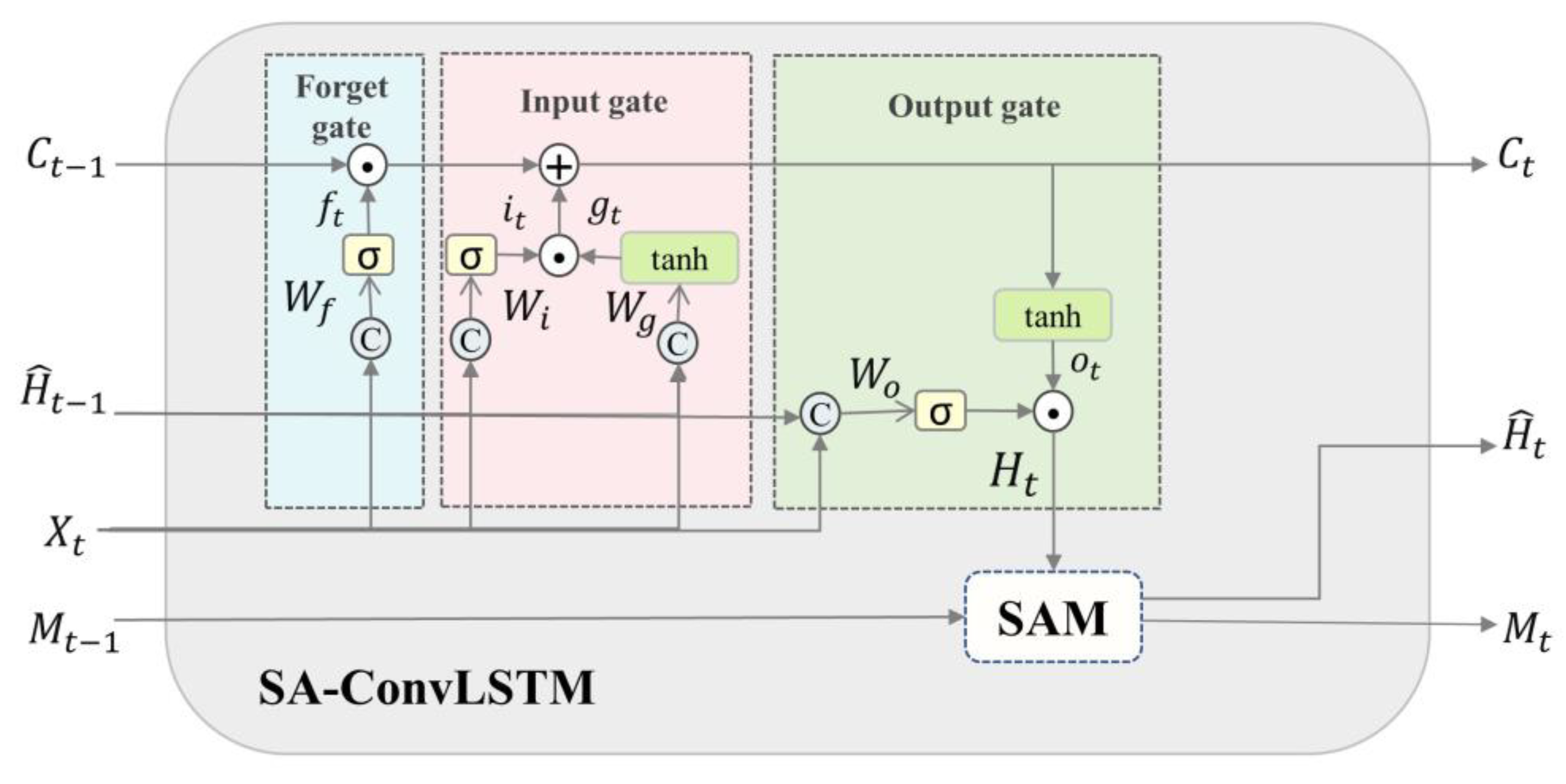
- SA-ConvLSTM
2.3.2. Computer Configuration and Parameter Settings
2.3.3. Evaluation Indictors
2.3.4. Method Flow
3. Results
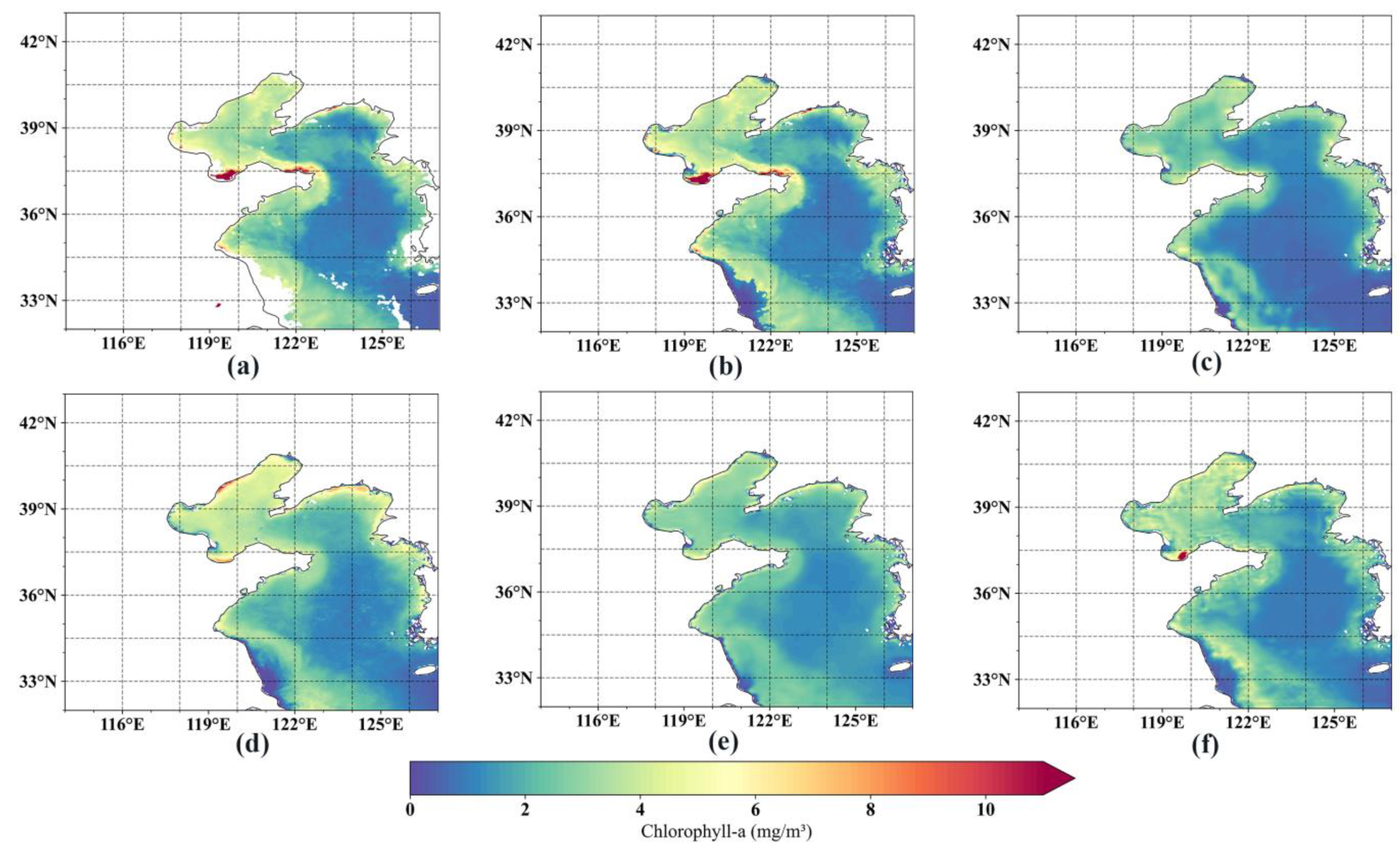
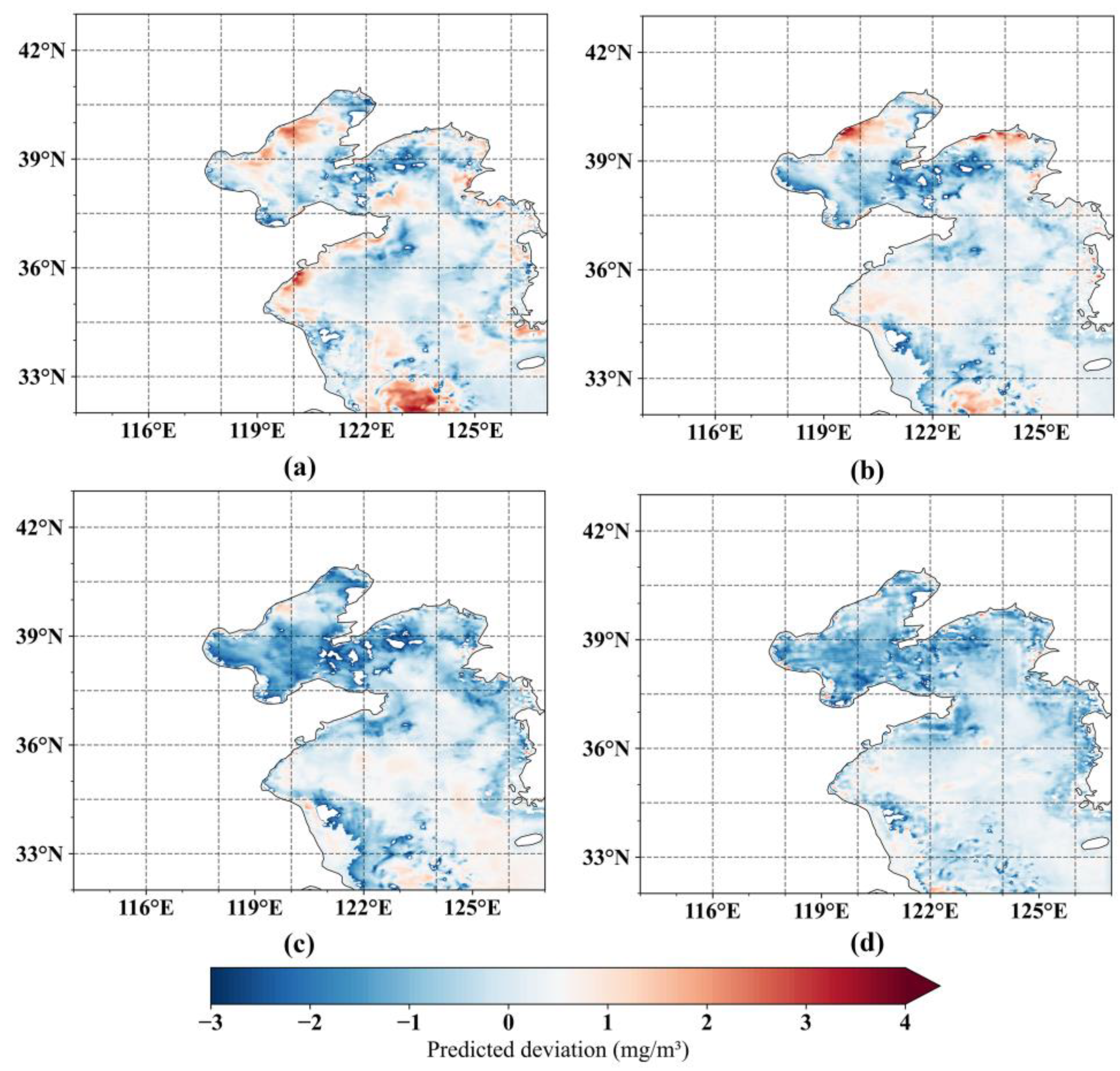
3.1. Spatial and Temporal Evaluation of Models for Predicting Chl-a
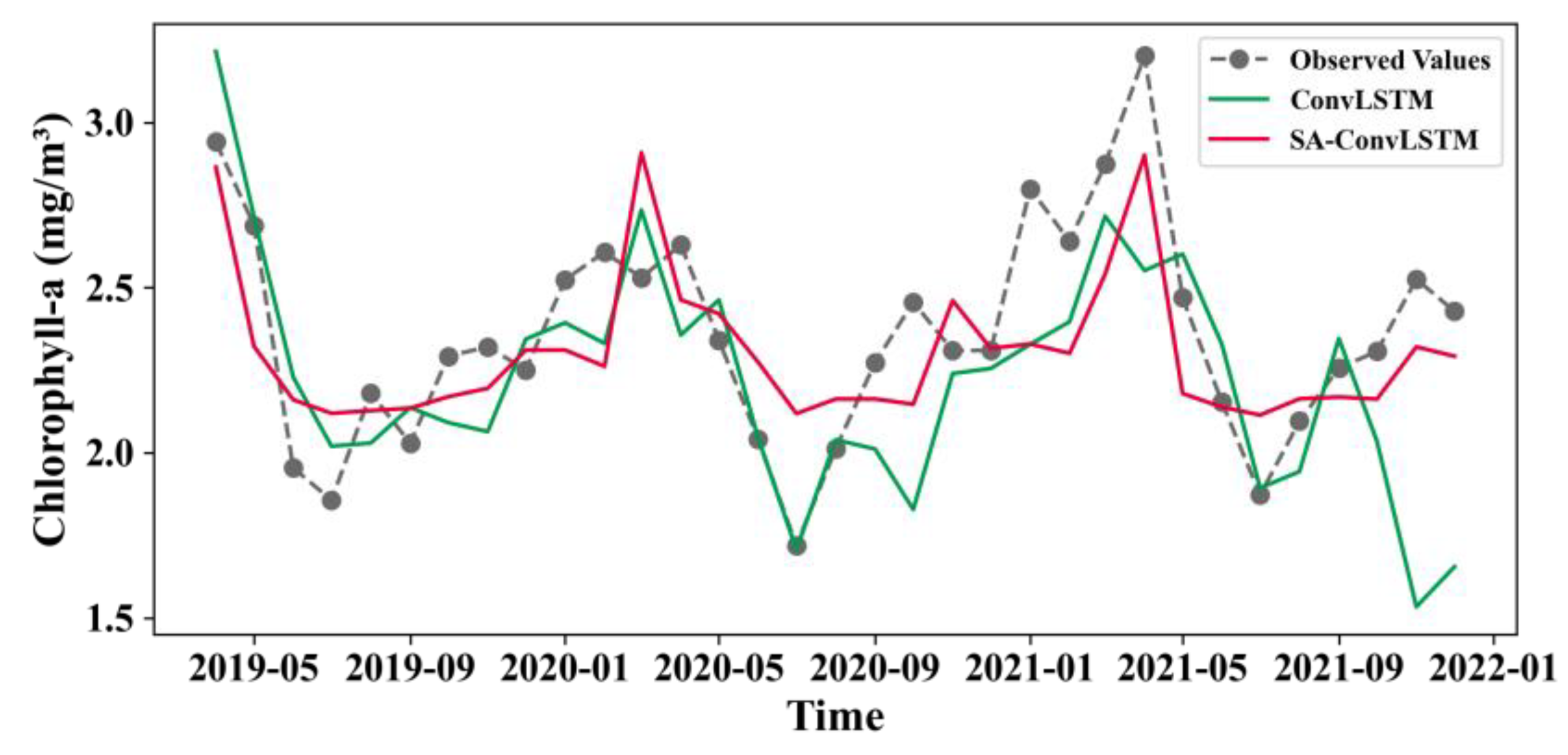
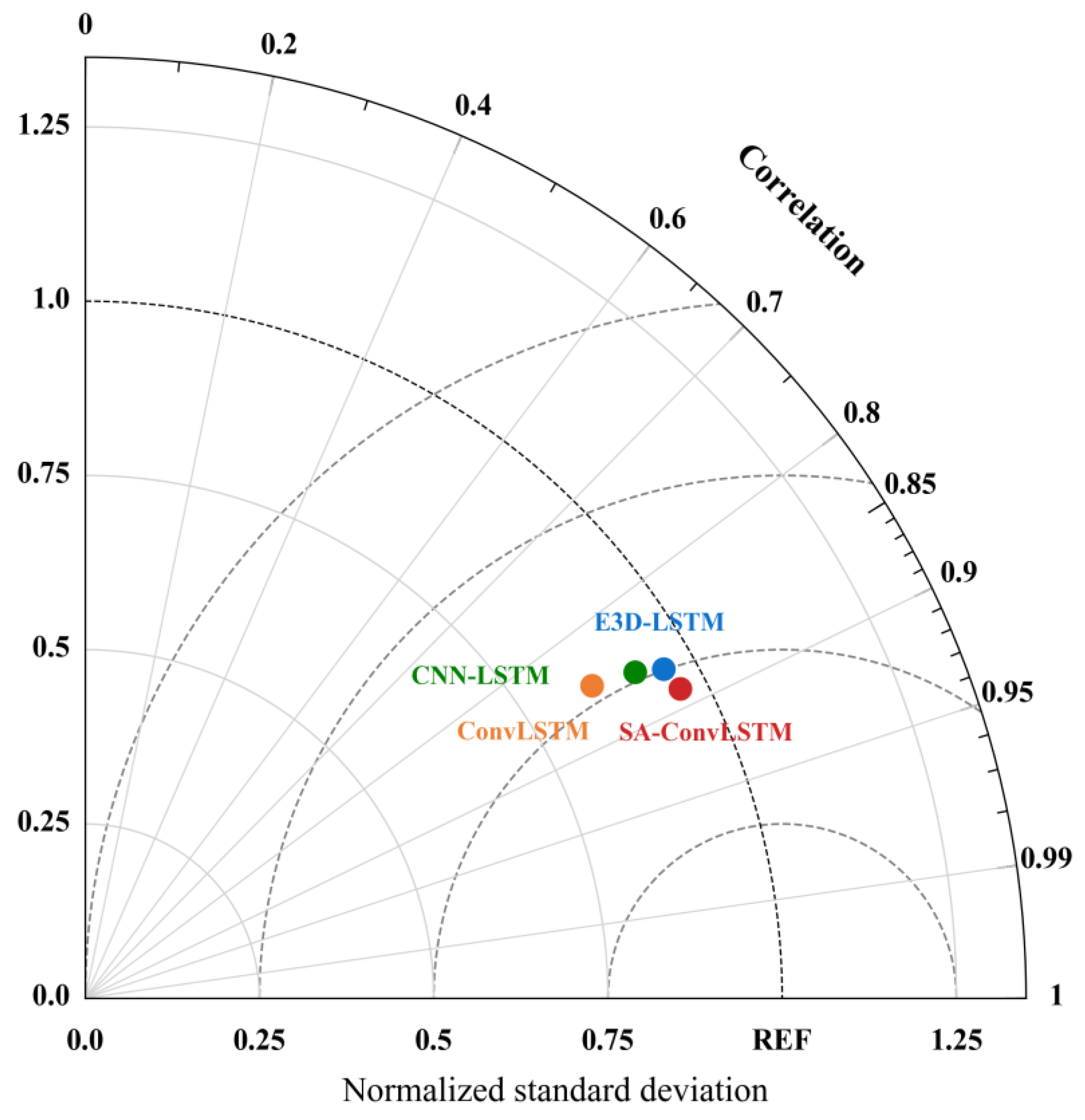
3.2. Performance Evaluation of Models for Predicting Chl-a
4. Discussion
5. Conclusions
Author Contributions
Funding
Data Availability Statement
Conflicts of Interest
References
- Sammartino, M.; Buongiorno Nardelli, B.; Marullo, S.; Santoleri, R. An Artificial Neural Network to Infer the Mediterranean 3D Chlorophyll-a and Temperature Fields from Remote Sensing Observations. Remote Sens. 2020, 12, 4123. [Google Scholar] [CrossRef]
- Zhao, N.; Zhang, G.; Zhang, S.; Bai, Y.; Ali, S.; Zhang, J. Temporal-Spatial Distribution of Chlorophyll-a and Impacts of Environmental Factors in the Bohai Sea and Yellow Sea. IEEE Access 2019, 7, 160947–160960. [Google Scholar] [CrossRef]
- Xing, M.; Yao, F.; Zhang, J.; Meng, X.; Jiang, L.; Bao, Y. Data reconstruction of daily MODIS chlorophyll-a concentration and spatio-temporal variations in the Northwestern Pacific. Sci. Total Environ. 2022, 843, 156981. [Google Scholar] [CrossRef]
- Wang, Y.; Gao, Z.; Liu, D. Multivariate DINEOF Reconstruction for Creating Long-Term Cloud-Free Chlorophyll-a Data Records From SeaWiFS and MODIS: A Case Study in Bohai and Yellow Seas, China. IEEE J. Sel. Top. Appl. Earth Obs. Remote Sens. 2019, 12, 1383–1395. [Google Scholar] [CrossRef]
- Cullen, J. The Deep Chlorophyll Maximum: Comparing Vertical Profiles of Chlorophyll a. Can. J. Fish. Aquat. Sci. 1982, 39, 791–803. [Google Scholar] [CrossRef]
- Fu, Y.; Xu, S.-g.; Liu, J. Temporal-spatial variations and developing trends of Chlorophyll-a in the Bohai Sea, China. Estuar. Coast. Shelf Sci. 2016, 173, 49–56. [Google Scholar] [CrossRef]
- Lu, X.; Liu, C.; Niu, Y.; Yu, S.X. Long-term and regional variability of phytoplankton biomass and its physical oceanographic parameters in the Yellow Sea, China. Estuar. Coast. Shelf Sci. 2021, 260, 107497. [Google Scholar] [CrossRef]
- Andersen, J.H.; Schlüter, L.; Ærtebjerg, G. Coastal eutrophication: Recent developments in definitions and implications for monitoring strategies. J. Plankton Res. 2006, 28, 621–628. [Google Scholar] [CrossRef]
- Cho, H.; Choi, U.J.; Park, H. Deep Learning Application to Time Series Prediction of Daily Chlorophyll-a Concentration. WIT Trans. Ecol. Environ. 2018, 215, 157–163. [Google Scholar]
- Barzegar, R.; Aalami, M.T.; Adamowski, J. Short-term water quality variable prediction using a hybrid CNN–LSTM deep learning model. Stoch. Environ. Res. Risk Assess. 2020, 34, 415–433. [Google Scholar] [CrossRef]
- Xiao, X.; He, J.; Huang, H.; Miller, T.R.; Christakos, G.; Reichwaldt, E.S.; Ghadouani, A.; Lin, S.; Xu, X.; Shi, J. A novel single-parameter approach for forecasting algal blooms. Water Res. 2017, 108, 222–231. [Google Scholar] [CrossRef]
- Li, X.; Sha, J.; Wang, Z.L. Application of feature selection and regression models for chlorophyll-a prediction in a shallow lake. Environ. Sci. Pollut. Res. Int. 2018, 25, 19488–19498. [Google Scholar] [CrossRef] [PubMed]
- Kiyomoto, Y.; Iseki, K.; Okamura, K. Ocean Color Satellite Imagery and Shipboard Measurements of Chlorophyll a and Suspended Particulate Matter Distribution in the East China Sea. J. Oceanogr. 2001, 57, 37–45. [Google Scholar] [CrossRef]
- Ndungu, J.; Monger, B.C.; Augustijn, D.C.M.; Hulscher, S.J.M.H.; Kitaka, N.; Mathooko, J.M. Evaluation of spatio-temporal variations in chlorophyll-a in Lake Naivasha, Kenya: Remote-sensing approach. Int. J. Remote Sens. 2013, 34, 8142–8155. [Google Scholar] [CrossRef]
- Cui, T.; Zhang, J.; Tang, J.; Sathyendranath, S.; Groom, S.; Ma, Y.; Zhao, W.; Song, Q. Assessment of satellite ocean color products of MERIS, MODIS and SeaWiFS along the East China Coast (in the Yellow Sea and East China Sea). ISPRS J. Photogramm. Remote Sens. 2014, 87, 137–151. [Google Scholar] [CrossRef]
- Meng, X.; Yao, F.; Zhang, J.; Liu, Q.; Liu, Q.; Shi, L.; Zhang, D. Impact of dust deposition on phytoplankton biomass in the Northwestern Pacific: A long-term study from 1998 to 2020. Sci. Total Environ. 2022, 813, 152536. [Google Scholar] [CrossRef]
- Vollenweider, R.A. Input-Output Models with Special Reference to the Phosphorus Loading Concept in Limnology. Schweiz. Z. Für Hydrol. 1975, 37, 53–84. [Google Scholar] [CrossRef]
- Jørgensen, S.E.; Mejer, H.; Friis, M. Examination of a lake model. Ecol. Model. 1978, 4, 253–278. [Google Scholar] [CrossRef]
- Box, G.E.P.; Jenkins, G.M.; Reinsel, G.C. Time Series Analysis: Forecasting and Control, 3rd ed.; Prentice Hall: Eng-lewood Cliffs, NJ, USA, 1994. [Google Scholar]
- Xiao, C.; Chen, N.; Hu, C.; Wang, K.; Xu, Z.; Cai, Y.; Xu, L.; Chen, Z.; Gong, J. A spatiotemporal deep learning model for sea surface temperature field prediction using time-series satellite data. Environ. Model. Softw. 2019, 120, 104502. [Google Scholar] [CrossRef]
- Zhou, S.; Xie, W.; Lu, Y.; Wang, Y.; Zhou, Y.; Hui, N.; Dong, C. ConvLSTM-Based Wave Forecasts in the South and East China Seas. Front. Mar. Sci. 2021, 8, 740. [Google Scholar] [CrossRef]
- Na, L.; Shaoyang, C.; Zhenyan, C.; Xing, W.; Yun, X.; Li, X.; Yanwei, G.; Tingting, W.; Xuefeng, Z.; Siqi, L. Long-term prediction of sea surface chlorophyll-a concentration based on the combination of spatio-temporal features. Water Res. 2022, 211, 118040. [Google Scholar] [CrossRef] [PubMed]
- Yu, B.; Xu, L.; Peng, J.; Hu, Z.; Wong, A. Global chlorophyll-a concentration estimation from moderate resolution imaging spectroradiometer using convolutional neural networks. J. Appl. Remote Sens. 2020, 14, 034520. [Google Scholar] [CrossRef]
- Yussof, F.N.; Maan, N.; Md Reba, M.N. LSTM Networks to Improve the Prediction of Harmful Algal Blooms in the West Coast of Sabah. Int. J. Environ. Res. Public Health 2021, 18, 7650. [Google Scholar] [CrossRef]
- Ham, Y.-G.; Kim, J.-H.; Luo, J.-J. Deep learning for multi-year ENSO forecasts. Nature 2019, 573, 568–572. [Google Scholar] [CrossRef] [PubMed]
- Ahmed, M.; Mumtaz, R.; Anwar, Z.; Shaukat, A.; Arif, O.; Shafait, F. A Multi–Step Approach for Optically Active and Inactive Water Quality Parameter Estimation Using Deep Learning and Remote Sensing. Water 2022, 14, 2112. [Google Scholar] [CrossRef]
- Shi, X.; Chen, Z.; Wang, H.; Yeung, D.Y.; Wong, W.K.; Woo, W.C. Convolutional LSTM Network: A Machine Learning Approach for Precipitation Nowcasting; MIT Press: Cambridge, MA, USA, 2015. [Google Scholar]
- Wang, Y.; Long, M.; Wang, J.; Gao, Z.; Philip, S.Y. PredRNN: Recurrent neural networks for predictive learning using spatiotem-poral LSTMs. In Proceedings of the Advances in Neural Information Processing Systems, Long Beach, CA, USA, 4–9 December 2017; pp. 879–888. [Google Scholar]
- Wang, Y.; Gao, Z.; Long, M.; Wang, J.; Yu, P.S. PredRNN++: Towards a Resolution of the Deep-in-Time Dilemma in Spatiotemporal Predictive Learning. In Proceedings of the 35th International Conference on Machine Learning, ICML 2018, Stockholm, Sweden, 15 July 2018; Volume 11, pp. 8122–8131. [Google Scholar]
- Wang, Y.; Lu, J.; Ming, H.Y.; Li, J.L.; Long, M.; Fei-Fei, L. Eidetic 3D LSTM: A Model for Video Prediction and Beyond. In Proceedings of the International Conference on Learning Representations, New Orleans, LA, USA, 6–9 May 2019. [Google Scholar]
- Lin, Z.; Li, M.; Zheng, Z.; Cheng, Y.; Yuan, C. Self-Attention Convlstm for Spatiotemporal Prediction. In Proceedings of the AAAI Conference on Artificial Intelligence, New York, NY, USA, 7–12 February 2020; The AAAI Press: Palo Alto, CA, USA, 2020; Volume 34, pp. 11531–11538. [Google Scholar]
- Luo, C.; Zhao, X.; Sun, Y.; Li, X.; Ye, Y. PredRANN: The spatiotemporal attention Convolution Recurrent Neural Network for precipitation nowcasting. Knowl.-Based Syst. 2022, 239, 107–109. [Google Scholar] [CrossRef]
- Wang, Y.; Wu, J.; Long, M.; Tenenbaum, J.B. Probabilistic Video Prediction From Noisy Data With a Posterior Confidence. In Proceedings of the 2020 IEEE/CVF Conference on Computer Vision and Pattern Recognition (CVPR), Seattle, WA, USA, 13–19 June 2020; pp. 10827–10836. [Google Scholar]
- Wu, H.; Yao, Z.; Long, M.; Wan, J. MotionRNN: A Flexible Model for Video Prediction with Spacetime-Varying Motions. In Proceedings of the 2021 IEEE/CVF Conference on Computer Vision and Pattern Recognition (CVPR), Nashville, TN, USA, 20–25 June 2021; pp. 15430–15439. [Google Scholar]
- Wang, Y.; Wu, H.; Zhang, J.; Gao, Z.; Wang, J.; Yu, P.S.; Long, M. PredRNN: A Recurrent Neural Network for Spatiotemporal Predictive Learning. IEEE Trans. Pattern Anal. Mach. Intell. 2021, 45, 2208–2225. [Google Scholar] [CrossRef]
- Natural Earth. Available online: https://www.naturalearthdata.com (accessed on 25 August 2023).
- OceanColor. Available online: https://oceancolor.gsfc.nasa.gov (accessed on 29 March 2022).
- Luo, X.; Song, J.; Guo, J.; Fu, Y.; Wang, L.; Cai, Y. Reconstruction of chlorophyll-a satellite data in Bohai and Yellow sea based on DINCAE method. Int. J. Remote Sens. 2022, 43, 3336–3358. [Google Scholar] [CrossRef]
- Zhai, F.; Wu, W.; Gu, Y.; Li, P.; Song, X.; Liu, P.; Liu, Z.; Chen, Y.; He, J. Interannual-decadal variation in satellite-derived surface chlorophyll-a concentration in the Bohai Sea over the past 16 years. J. Mar. Syst. 2020, 215, 103496. [Google Scholar] [CrossRef]
- Volpe, G.; Nardelli, B.B.; Cipollini, P.; Santoleri, R.; Robinson, I.S. Seasonal to interannual phytoplankton response to physical processes in the Mediterranean Sea from satellite observations. Remote Sens. Environ. 2012, 117, 223–235. [Google Scholar] [CrossRef]
- Behrenfeld, M.J.; Falkowski, P.G. Photosynthetic rates derived from satellite-based chlorophyll concentration. Limnol. Oceanogr. 1997, 42, 1–20. [Google Scholar] [CrossRef]
- Gong, G.-C.; Liu, K.-K. The Relationship Between Surface Chlorophyll a and Biogenic Matter in the Euphotic Zone in the Southern East China Sea in Spring. COSPAR Colloquia Ser. 1997, 8, 175–178. [Google Scholar]
- Gupta, G.V.M.; Sudheesh, V.; Sudharma, K.V.; Saravanane, N.; Dhanya, V.; Dhanya, K.R.; Lakshmi, G.; Sudhakar, M.; Naqvi, S.W.A. Evolution to decay of upwelling and associated biogeochemistry over the southeastern Arabian Sea shelf. J. Geophys. Res. Biogeosciences 2016, 121, 159–175. [Google Scholar] [CrossRef]
- Liang, Z.; Soranno, P.A.; Wagner, T. The role of phosphorus and nitrogen on chlorophyll a: Evidence from hundreds of lakes. Water Res. 2020, 185, 116236. [Google Scholar] [CrossRef]
- Beckers, J.M.; Barth, A.; Alvera-Azcárate, A. DINEOF reconstruction of clouded images including error maps. Application to the Sea-Surface Temperature around Corsican Island. Ocean Sci. 2006, 2, 183–199. [Google Scholar] [CrossRef]
- Prasetyowati, S.A.D.; Ismail, M.; Budisusila, E.N.; Setiadi, D.R.I.M.; Purnomo, M.H. Dataset Feasibility Analysis Method based on Enhanced Adaptive LMS method with Min-max Normalization and Fuzzy Intuitive Sets. Int. J. Electr. Eng. Inform. 2022, 14, 55–75. [Google Scholar] [CrossRef]
- Szegedy, C.; Liu, W.; Jia, Y.; Sermanet, P.; Reed, S.; Anguelov, D.; Erhan, D.; Vanhoucke, V.; Rabinovich, A. Going deeper with convolutions. In Proceedings of the IEEE Conference on Computer Vision and Pattern Recognition, Boston, MA, USA, 7–12 June 2015; pp. 1–9. [Google Scholar]
- Nogueira, K.; Penatti, O.; Santos, J. Towards Better Exploiting Convolutional Neural Networks for Remote Sensing Scene Classification. Pattern Recognit. 2016, 61, 539–556. [Google Scholar] [CrossRef]
- Vaswani, A.; Shazeer, N.; Parmar, N.; Uszkoreit, J.; Jones, L.; Gomez, A.N.; Kaiser, L.; Polosukhin, I. Attention Is All You Need. In Proceedings of the Advances in Neural Information Processing Systems 30, Long Beach, CA, USA, 4–9 December 2017; pp. 5998–6008. [Google Scholar]
- Ge, H.; Li, S.; Cheng, R.; Chen, Z. Self-Attention ConvLSTM for Spatiotemporal Forecasting of Short-Term Online Car-Hailing Demand. Sustainability 2022, 14, 7371. [Google Scholar] [CrossRef]
- Jacobs, R.A. Increased Rates of Convergence Through Learning Rate Adaptation. Neural Netw. 1988, 1, 295–307. [Google Scholar] [CrossRef]
- Donahue, J.; Hendricks, L.A.; Rohrbach, M.; Venugopalan, S.; Guadarrama, S.; Saenko, K.; Darrell, T. Long-Term Recurrent Convolutional Networks for Visual Recognition and Description. IEEE Trans. Pattern Anal. Mach. Intell. 2017, 39, 677–691. [Google Scholar] [CrossRef]
- Nair, V.; Hinton, G.E. Rectified Linear Units Improve Restricted Boltzmann Machines. In Proceedings of the 27th International Conference on Machine Learning (ICML-10), Haifa, Israel, 21–24 June 2010; pp. 807–814. [Google Scholar]
- Girosi, F.; Jones, M.; Poggio, T. Regularization Theory and Neural Networks Architectures. Neural Comp. 1995, 7, 219–269. [Google Scholar] [CrossRef]
- Ghorbani, M.A.; Deo, R.C.; Karimi, V.; Yaseen, Z.M.; Terzi, O. Implementation of a hybrid MLP-FFA model for water level prediction of Lake Egirdir, Turkey. Stoch. Environ. Res. Risk Assess. 2018, 32, 1683–1697. [Google Scholar] [CrossRef]
- Paerl, H.; Otten, T. Harmful Cyanobacterial Blooms: Causes, Consequences, and Controls. Microb. Ecol. 2013, 65, 995–1010. [Google Scholar] [CrossRef] [PubMed]
- Zhang, H.; Qiu, Z.; Sun, D.; Wang, S.; He, Y. Seasonal and Interannual Variability of Satellite-Derived Chlorophyll-a (2000–2012) in the Bohai Sea, China. Remote Sens. 2017, 9, 582. [Google Scholar] [CrossRef]


| Parameter | Description | Unit | Spatial Resolution | Temporal Resolution | Data Source |
|---|---|---|---|---|---|
| Chl-a | Chlorophyll-a Concentrations | mg/m3 | 4 km × 4 km | Monthly | OceanColor |
| PIC | Particulate Inorganic Carbon | mol/m3 | |||
| POC | Particulate Organic Carbon | mol/m3 | |||
| SST | Sea Surface Temperature | degree_C | |||
| PAR | Photosynthetically Available Radiation | einstein/m2/day | |||
| NFLH | Normalised Fluorescence Line Height | W/m2/um/sr | |||
| U10 | 10 Metre U Wind Component | m/s | 0.25° × 0.25° | Monthly | ERA5 |
| V10 | 10 Metre V Wind Component | m/s | |||
| T2M | 2 Metre Temperature | K | |||
| SP | Surface Pressure | Pa | |||
| TP | Total Precipitation | m | |||
| MSL | Mean Sea Level Pressure | Pa | 0.5° × 0.5° | Monthly | ERA5 |
| SWH | Significant Height of Combined Wind Waves and Swell | m | |||
| MWD | Mean Wave Direction | Degree | 1° × 1° | Monthly | ERA5 |
| MWP | Mean Wave Period | s |
| Period | Deep Learner | r | MAE | MSE | RMSE |
|---|---|---|---|---|---|
| Training period | ConvLSTM | 0.827 | 0.250 | 0.669 | 0.818 |
| CNN-LSTM | 0.849 | 0.205 | 0.580 | 0.762 | |
| E3D-LSTM | 0.860 | 0.208 | 0.555 | 0.745 | |
| SA-ConvLSTM | 0.879 | 0.227 | 0.540 | 0.735 | |
| Testing period | ConvLSTM | 0.851 | 0.232 | 0.656 | 0.810 |
| CNN-LSTM | 0.860 | 0.218 | 0.518 | 0.719 | |
| E3D-LSTM | 0.869 | 0.206 | 0.495 | 0.704 | |
| SA-ConvLSTM | 0.887 | 0.212 | 0.482 | 0.687 |
| Performance Evaluation | ConvLSTM | CNN-LSTM | E3D-LSTM | SA-ConvLSTM |
|---|---|---|---|---|
| Number of parameters (M) | 1.066 | 328.531 | 111.709 | 1.908 |
| Time/Epoch (s) | 12.189 | 8.615 | 1513.579 | 16.900 |
| Dropped Feature | r | MAE | MSE | RMSE |
|---|---|---|---|---|
| U10 | 0.886 | 0.213 | 0.487 | 0.690 |
| V10 | 0.884 | 0.215 | 0.489 | 0.691 |
| MWD | 0.876 | 0.218 | 0.554 | 0.734 |
| MWP | 0.877 | 0.226 | 0.514 | 0.709 |
| SWH | 0.876 | 0.209 | 0.548 | 0.730 |
| TP | 0.876 | 0.213 | 0.551 | 0.733 |
| U10, V10 | 0.878 | 0.206 | 0.542 | 0.727 |
| MWD, TP, MWP, SWH | 0.875 | 0.211 | 0.553 | 0.734 |
| Non-Removal | 0.887 | 0.212 | 0.482 | 0.687 |
Disclaimer/Publisher’s Note: The statements, opinions and data contained in all publications are solely those of the individual author(s) and contributor(s) and not of MDPI and/or the editor(s). MDPI and/or the editor(s) disclaim responsibility for any injury to people or property resulting from any ideas, methods, instructions or products referred to in the content. |
© 2023 by the authors. Licensee MDPI, Basel, Switzerland. This article is an open access article distributed under the terms and conditions of the Creative Commons Attribution (CC BY) license (https://creativecommons.org/licenses/by/4.0/).
Share and Cite
Yao, L.; Wang, X.; Zhang, J.; Yu, X.; Zhang, S.; Li, Q. Prediction of Sea Surface Chlorophyll-a Concentrations Based on Deep Learning and Time-Series Remote Sensing Data. Remote Sens. 2023, 15, 4486. https://doi.org/10.3390/rs15184486
Yao L, Wang X, Zhang J, Yu X, Zhang S, Li Q. Prediction of Sea Surface Chlorophyll-a Concentrations Based on Deep Learning and Time-Series Remote Sensing Data. Remote Sensing. 2023; 15(18):4486. https://doi.org/10.3390/rs15184486
Chicago/Turabian StyleYao, Lulu, Xiaopeng Wang, Jiahua Zhang, Xiang Yu, Shichao Zhang, and Qiang Li. 2023. "Prediction of Sea Surface Chlorophyll-a Concentrations Based on Deep Learning and Time-Series Remote Sensing Data" Remote Sensing 15, no. 18: 4486. https://doi.org/10.3390/rs15184486