Article

Non-Local SAR Image Despeckling Based on Sparse Representation

1
School of Information Engineering, China University of Geosciences (Beijing), Beijing 100083, China
2
School of Electronic and Information Engineering, Beihang University, Beijing 100191, China
*
Author to whom correspondence should be addressed.
Remote Sens. 2023, 15(18), 4485; https://doi.org/10.3390/rs15184485
Submission received: 15 August 2023 / Revised: 8 September 2023 / Accepted: 10 September 2023 / Published: 12 September 2023
(This article belongs to the Special Issue Advance in SAR Image Despeckling)

Abstract

:
Speckle noise is an inherent problem of synthetic aperture radar (SAR) images, which not only seriously affects the acquisition of SAR image information, but also greatly reduces the efficiency of image segmentation and feature classification. Therefore, research on how to effectively suppress speckle noise while preserving SAR image content information as much as possible has received increasing attention. Based on the non-local idea of SAR image block-matching three-dimensional (SAR-BM3D) algorithm and the concept of sparse representation, a novel SAR image despeckling algorithm is proposed. The new algorithm uses K-means singular value decomposition (K-SVD) to learn the dictionary to distinguish valid information and speckle noise and constructs a block filter based on K-SVD for despeckling, so as to avoid strong point diffusion problem in SAR-BM3D and achieve better speckle noise suppression with stronger adaptability. The experimental results on real SAR images show that the proposed algorithm achieves better comprehensive effect of speckle noise suppression in terms of evaluation indicators and information preservation of SAR images compared with several existing algorithms.

Graphical Abstract

1. Introduction

According to the roughness of the image, synthetic aperture radar (SAR) images can be divided into three regions: homogeneous region, heterogeneous region, and extreme heterogeneous region. The scattering in homogeneous regions is relatively balanced, such as grassland and sea surface. Heterogeneous regions contain features such as edges and textures, while extreme heterogeneous regions often contain targets such as strong scatterers. Due to the randomness of the scatterer in spatial distribution and backscattering characteristics, the amplitude and phase of the echoes of the resolution unit also have randomness. Even in homogeneous regions where the backscattering characteristics of the scatterers are basically the same, the intensity of the echoes from different resolving units may be different, which leads to the fluctuation of the intensity of the imaging results and the formation of coherent speckle noise [1]. The coherent speckle noise causes the signal intensity between adjacent pixels to change, which visually manifests as granular noise, i.e., speckle noise. Speckle noise seriously affects the acquisition and application of SAR image information. Therefore, speckle noise suppression has been a hot spot in the field of SAR image processing research.
Early traditional filtering algorithms, such as space-domain filtering [2,3,4,5,6], transform-domain filtering [7,8], and partial differential equation filtering (PDE) [9,10,11], are well developed. All these methods estimate the local statistics of the image with convenient process and high real-time performance. However, there are certain limitations in maintaining detailed texture. Since then, the non-local mean (NLM) filtering algorithm [12,13] has made great progress. The basic idea is to select a search window centered on the filtered pixel, calculate the similar weights of the pixels in the search window and the filtered pixel, and then weigh the sum of all pixels in the window and their corresponding similar weights to obtain the filtered pixel’s filtering result. Compared with the traditional filter, the non-local mean filter makes full use of the similarity of image pixels, has stronger adaptivity, and can effectively avoid the generation of artifacts. Therefore, the non-local mean filter is currently the most widely used in the field of speckle noise suppression and has the best comprehensive effect.
In 2007, Dabov et al. proposed the block-matching three-dimensional (BM3D) algorithm by combining the ideas of non-local mean filtering and joint filtering [14]. BM3D shows excellent denoising ability on optical images. Later, Sara Parrilli et al. changed the similarity calculation method in BM3D to the similarity weight calculation method in the Probabilistic patch-based (PPB) algorithm and the joint filtering method to linear minimum mean square error filtering on wavelet domain and proposed the SAR-BM3D despeckling algorithm applicable to SAR images [15]. The SAR image block-matching three-dimensional algorithm (SAR-BM3D) shows good speckle noise suppression performance and edge retention ability and is currently recognized as one of the best methods for SAR image despeckling. Generally speaking, denoising means noise removal of optical images, and despeckling means the speckle noise suppression of SAR images. However, when the speckle noise intensity is too large, the calculation accuracy of similar weights in the non-local similar block-matching process will be affected and strong point diffusion phenomenon will be generated.
To solve this problem, a new non-local SAR image despeckling method based on sparse representation is proposed in this paper. The core idea of this new method is to use sparsity and maximum posterior estimation methods for despeckling, which can distinguish effective terrain information from unstructured speckle noise in the image. This can effectively avoid the problem of strong point diffusion in SAR-BM3D. The approximate process is to follow the first step of coarse filtering of SAR-BM3D. The second step of fine filtering is to use K-means singular value decomposition (K-SVD) sparse representation image despeckling [16] instead of minimum linear mean square deviation filtering on the logarithmic image of the coarse filtered image. As the residual between the original image and the reconstructed image in the process of dictionary iterative learning and image reconstruction, the nonstructural information in the image, i.e., speckle noise, can be discarded during dictionary iterative learning and image reconstruction processes.
The organization of this paper is as follows. In Section 2, the principle of sparse representation despeckling and the basic idea of the proposed algorithm are introduced in detail. The specific flow of the proposed algorithm is described in detail in Section 3. The experimental results of real SAR images are shown in Section 4 to demonstrate the effectiveness of the proposed algorithm. And the conclusion is given in Section 5.

2. Basic Idea

The basic idea of this article is to integrate sparse representation denoising into non-local mean filtering in theory and algorithm structure. In this section, the model of speckle noise in SAR images is first analyzed, followed by an introduction to sparse representation theory and related image-denoising algorithms. Finally, the motivation of applying sparse representation theory to non-local filtering in the new algorithm is explained in detail.

2.1. Noise Model Analysis

In optical images, noise usually exists in additive form. In contrast, speckle noise satisfies the multiplicative model under the assumption of full development. The noise-free optical image and the image after adding multiplicative noise are shown in Figure 1. Assuming that the coherent speckle noise of the SAR image is fully developed, the observed SAR image I can be represented by the following model [17]:
I = xv,
where x is the true speckle-free SAR image and v is the coherent speckle noise. A Gamma distribution with mean 1/L and variance 1/L is obeyed, where L is the number of image views. The common denoising algorithms designed for additive noise cannot be applied to SAR images directly. As a result, logarithmic conversion of the SAR image is required before despeckling. The SAR image model is converted to an additive model. The image model is then transformed into the following model:
I ~ = log ( I ) = log ( x ) + log ( v ) = X ~ + V ~ ,
SAR image can be regarded as the superposition of valid information and speckle noise. The valid information refers to the part of the image that can provide the information of the observed scene, such as terrain, buildings, maneuvering targets. In SAR-BM3D algorithm, speckle noise appears in the form of disordered and random high-intensity pixels in the similar block-matching step. When the intensity of speckle noise in SAR images is too high, it is possible to match two randomly similar blocks of noisy pixel blocks into a similar block group. This actually enhances the noise pixels in the subsequent joint filtering, resulting in strong point diffusion phenomenon and even false targets. The key to solving this problem is to enable the algorithm to distinguish whether the pixels in an image belong to valid information or speckle noise. The valid information in the SAR image tends to have a certain structure and texture, while the speckle noise is disordered and random. It is due to the different sparsity of the valid information and speckle noise that the human eye can distinguish between them in the image. This sparsity is the key to solving the problem of strong scatterer diffusion.

2.2. Sparse Representation

Transform dictionaries are usually divided into general dictionaries and learning dictionaries. Common general dictionaries choose the fixed form dictionaries on specific transform domain, such as Fourier transform (FT) dictionary, discrete cosine transform (DCT) dictionary, wavelet transform (WT) dictionary, contourlet dictionary, etc. The learning dictionary is a special dictionary generated by training the image to be processed. Each column in the dictionary is called an atom, each atom contains the structural features of the image. Sparse representation theory assumes that signals can be represented by linear combination of a finite number of atoms in a predefined dictionary. The coefficients corresponding to these atoms are the combination coefficients. Most of the combination coefficients are approximately zero. The matrix formed by these combination coefficients is the coefficient matrix. The coefficient matrix is sparse. After constructing the sparse linear model using the training samples, the atoms are endowed with the structure features of the valid information. The valid information in the image can be obtained from a finite number of atoms in the dictionary. The valid information can be combined linearly by these finite atoms with the sparse coefficient matrix.
As illustrated in Figure 2, given an image X, valid information such as terrain information in X can be expressed as the product of a dictionary D and a sparse coefficient matrix α, i.e., X = Dα. The randomness and unstructured nature of the invalid information prevents it from being represented sparsely by the dictionary [18]. Therefore, for a noise-containing image X, which will be reconstructed by the dictionary and the sparse coefficient matrix, the noise in X will not be sparsely represented. The reconstructed image X = Dα contains only the valid information in the original image X, and the noise will be discarded as the residual (X − X ). This is the basic principle: that the sparse representation can denoise the image.
The original representation filtering on specific transform domain sets a threshold for the coefficient matrix by a specific shrinkage method. The elements of the coefficient matrix less than the threshold are regarded as zero, and the coefficient items containing noise are discarded. Denoising is accomplished by exploiting the sparsity of the coefficient matrix on this specific transform domain. The most classical hard threshold shrinkage is to set a threshold artificially, and the elements below the threshold are counted as near-zero, then the coefficient matrix can be regarded as sparse. The original sparse representation filtering on a specific transform domain extracts a finite number of atom combinations in the corresponding orthogonal dictionary of this transform domain. Then, the denoised results are reconstructed by inverse transformation. The coefficient items containing noise information are discarded as reconstruction residuals in this process. This idea has led to the creation of the well-known wavelet shrinkage algorithm and several new customized multi-scale and directional redundant transformation, such as [19,20]. These algorithms are easy to understand and operate.
However, the success of such a general dictionary approach in practical denoising applications depends on whether the filtered signal is sparse in the corresponding transform domain. Therefore, this kind of method is not sufficiently general. Compared with the specific transform domain filtering, the sparse despeckling part of the new proposed algorithm takes the form of solving the maximum a posteriori (MAP) estimation problem. The dictionary of the new proposed method is a set of learned parameters learned from the image instead of the set of pre-selected basis functions like curvelet or contourlet. The DCT dictionary is used as the initial dictionary. In each iteration, the orthogonal matching pursuit (OMP) [21] method is used to update the sparse coefficient matrix row by row, and the singular value decomposition is used to update the dictionary matrix column by column. The optimal solution that meets the constraints is learned from multiple optimizations. The constraints are usually divided into sparsity constraint and image error constraint. The sparsity constraint is the maximum sparsity of the coefficient matrix, image error constraint is the maximum error between the input image and the reconstructed image. Dictionary learning is an iterative process of optimizing the dictionary column by column using an update method in each iteration. The sparse representation is the process in which the reconstructed image is linearly combined by using updated dictionary with updated sparse coefficient matrix in each optimization process.
The effect of the maximum a posteriori estimation method is related to the degree of dictionary quality optimization. In this paper, the degree of sparsity is defined as the ratio of the number of non-zero elements to the total number of elements in a column of atoms in the dictionary. As shown in Figure 3 and Figure 4, Figure 3 shows that the dictionary learned from real SAR images with different number of iterations, (a) is the dictionary learned from iteratively updating five times, and (b) is the dictionary learned from iteratively updating ten times. Figure 4 shows the despeckling results learned from real SAR images with different number of iterations, (a) is the despeckling result learned from iteratively updating five times, and (b) is the despeckling result learned from iteratively updating ten times. Obviously, the filtering results (a) in the Figure 4 corresponding to the dictionary learned from five iterations are fuzzy, the point targets are mixed together, and the experimental data show that the sparsity degree of the learned sparse coefficient matrix learned from five iterations is 9/256. Compared with the filtering results after five iterations in Figure 4a, the filtering results after ten iterations in Figure 4b are significantly more detailed, and the edge and point targets marked by red rectangles are also clearer. The experimental data show that the sparsity degree of the sparse coefficient matrix learned from ten iterations is reduced to 3/256. Therefore, with the increase in the number of iterations, the quality of the learned dictionary can be gradually improved. The learned dictionary after more iterations can not only express more detailed parts of the image, but also reduce the sparsity degree of the sparse matrix. As a result, it can be seen from Figure 3 and Figure 4 that the dictionary optimized with a larger number of iterations has the potential to represent the image more accurately and sparsely.
Inspired by the above conclusion that the higher the number of iterative updates, the higher the quality of the learned dictionary, the proposed method uses the sparse representation filtering based on K-SVD to accomplish the filtering in specific transform domain. The optimal dictionary and sparse coefficient matrix that satisfy the constraints are learned, so as to achieve the best combined effect of speckle noise suppression and image detail representation. K-SVD based on overcomplete dictionary learning is one of the most representative algorithms in image denoising based on sparse representation. Then, SAR image filtering based on dictionary learning and sparse representation [22] adds a pre-processing step of logarithmic conversion of the image before K-SVD image despeckling. The SAR image-denoising model based on weighted sparse representation [23,24] performs similar block matching on the logarithmic image of the original SAR image, and then performs K-SVD image denoising. This SAR image filtering based on dictionary learning and sparse representation applies the sparse representation filtering idea to SAR image despeckling, showing good results in speckle noise suppression.

2.3. Motivation

The core idea of K-SVD filtering is to take advantage of the different characteristics that valid information can be sparsely represented, while noise information cannot be sparsely represented. The different characteristics can precisely help to solve the problem that valid information and noise in the image are difficult to distinguish in amplitude. From the perspective of algorithm structure, the image denoising based on sparse representation has some similarity with the method architecture in SAR-BM3D. They both contain the steps of image block selection, filter processing, and block restoration. So, the block filtering step of fine filtering in SAR-BM3D can be theoretically replaced by K-SVD despeckling. A new algorithm of non-local SAR image despeckling based on sparse representation can be proposed.
The proposed algorithm does not have a serious impact on the filtering results during the similar block-matching process, even if the similar block matching is affected by the high-intensity speckle noise. Since the speckle noise of the image is still unstructured and cannot be represented sparsely by the dictionary, the speckle noise will be discarded during the reconstruction of the image through the dictionary and sparse coefficient matrix.
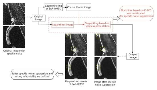
The first step of the new algorithm follows the coarse filtering step of SAR-BM3D. The second step is performed on the logarithmic image of the original image. The logarithmic image is divided into blocks of the same size to form a three-dimensional dictionary group. And the dictionary of the corresponding block is selected according to the position of the current image block in the filtering process. Then, the sparse matrix and learned dictionary are trained using the OMP method and K-SVD. Finally, the filtered image blocks are reconstructed. The K-SVD algorithm is flexible and can be used with a variety of pursuit methods, the classical OMP pursuit method is selected in this paper. After sequentially and iteratively processing all image blocks, the final image is restored by weight aggregation. Such an improvement not only inherits the strong adaptivity and good filtering effect of SAR-BM3D, but also can overcome the drawback of strong point diffusion for strong noise images and demonstrate the adaptability of the algorithm. The specific method flow will be described in detail in Section 3.

3. Proposed Algorithm

The overall flowchart of the proposed algorithm is shown in Figure 5. The first part marked in blue color in Figure 5, follows the architecture of SAR-BM3D, which performs coarse filtering on the original image I. The coarse filtering process is made up of similar block matching, undecimated discrete wavelet transform (UDWT) filtering based on local linear minimum-mean-square-error (LLMMSE) shrinkage, and aggregation.
Since the original K-SVD denoising is suitable to deal with additive noise and the speckle noise is the multiplicative model, the original image needs to be log-transformed before the second part begins. In the second part marked in red color in Figure 5, similar block matching is performed again on the coarse filtered output image. As shown in Figure 6, the similar blocks in the corresponding position in the logarithmic image I l o g are converted into one-dimensional column data. As shown in Figure 7, the reference block marked in yellow color is the image block at the current filtering position. In a certain selection region marked in blue color centered on the reference block, the similarity between the reference block and each image block in this selection region is calculated. The image blocks with large similarity are the similar blocks of the reference block, which is marked in red color. All the blocks similar to the same reference block form a similar block group. Each image block in a similar block group is converted into one-dimensional column data, which are stacked into a two-dimensional matrix Y G by column. After the DCT dictionary is determined as the initial dictionary, the OMP tracking method and K-SVD are used to update and learn the three-dimensional dictionary group and sparse coefficient matrix. The iterative update was performed until the sparse matrix met the set sparse depth range and the image met the set error range. The reconstructed image of the last iteration is the logarithmic image block after sparse representation despeckling. Then, the filtered logarithmic image blocks are aggregated and restored according to the weight. The final despeckling image is obtained by exponentiating the aggregated logarithmic image.

3.1. Three-Dimensional Dictionary Group

After completing the first step of coarse filtering on the original image, similar block matching needs to be performed again on the coarse filtered image. Since SAR images are generally too large, the learning dictionary far away from the selection region of reference block is not structurally representative for the reference block. Moreover, dictionary learning is very time-consuming. However, if a selection region is randomly selected for dictionary learning, it is easy to miss the region near the reference block, which makes the learned dictionary invalid for the reference block.
Therefore, in the dictionary training step, the proposed algorithm makes some improvements. Different from the original K-SVD denoising algorithm, the logarithmic image of the coarse filtering result is divided into image blocks of the same size: each image block is transformed separately to obtain the initial dictionary, so as to obtain a three-dimensional dictionary group. When the dictionary needs to be trained or used, the corresponding dictionary is selected according to the position of the reference block for updating or reconstruction. In this way, the dictionary set obtained by training can be more representative of the local structure for the reference block, which can effectively reduce the generation of reconstructed image artifacts. As the commonly used dictionary [25,26], the DCT dictionary is selected as the initialization dictionary in this proposed method.

3.2. Sparse Representation Despeckling

The image despeckling part, based on sparse representation of the new algorithm, updates the dictionary and the sparse matrix iteratively by using the K-SVD method and the pursuit method. The K-SVD method has very strong applicability and can be combined with a variety of pursuit methods, and the classical OMP pursuit method is used in this paper, so as to solve the equation:
α j ^ = a r g m i n α 0 , s . t . X j D j α j F 2 < n c ε ,
D j is the dictionary corresponding to the current reference block in the three-dimensional dictionary group. α j ^ is the sparsity coefficient matrix corresponding to the dictionary D j . The first term α 0 is the sparsity constraint, the second term X j D j α j F 2 is the error between the two-dimensional matrix Y G and the reconstructed two-dimensional matrix Y G ^ , n c is the number of columns of the two-dimensional matrix Y G , and ε is the maximum allowed value of the reconstruction error. When the sparsity and image error constraints are satisfied or the maximum number of iterations was reached, the reconstructed image of the last iteration was output.
The above operation is the filtering process of one reference block and its similar block group. For the filtering of the whole image, this process needs to be carried out by traversing all image blocks in turn. Y G ^ is the filtered value of the two-dimensional matrix Y G after sparse representation despeckling. Y G ^ is restored as y p a t c h ^ , y p a t c h ^ is reconstructed image block of the reference block or its similar blocks. y p a t c h is the reference block or its similar blocks. Then, all the y p a t c h ^ are aggregated and restored to the original position with a certain weight.
For the whole image, the filtering values of the same pixel in different similar block groups are aggregated by the weight summation in the SAR-BM3D algorithm. x ^ G ( s ) is the value of pixel s in a group of estimates values. w G is the weight of this group of estimate values in the aggregation restoration process. The pixel value x(s) of the final result is:
x s = s Y G w G x ^ G ( s ) s Y G w G ,
The weights w G are obtained by the following formula:
w G 1 E ( n 2 ) 1 E [ ( y p a t c h y p a t c h ^ ) 2 ] ,
where E[·] denotes statistical expectation, n 2 is the variance between the y p a t c h and its reconstructed image block y p a t c h ^ . E [ ( y p a t c h y p a t c h ^ ) 2 ] is the variance expectation of all image blocks in a similar block group. The larger the variance, the smaller the weight of these filtering values. The process is repeated to traverse the whole image in turn, and the final despeckled image is obtained by exponentiating the whole image.

4. Experimental Result

In order to verify the effectiveness of the proposed algorithm, experiments based on real SAR images in TerraSAR-X measured data and simulation images are performed in this section. In this experiment, the real SAR images are filtered by various classical speckle noise suppression methods and the proposed method. The equivalent number of looks (ENL), the edge preservation indicator (EPI) and the ratio of the original image and the despeckled image R are used to evaluate and compare the filtering effect in homogeneous region, edge preservation effect, and overall information preservation ability of the image.

4.1. Parameter Setting

For all the algorithms performed in the experiments, the parameters are set as suggested in the references if not stated otherwise. In the coarse filtering step of the proposed algorithm, the size of the similar block group is fixed as 8 × 8 × 16, and the size of search window is 39 × 39, which is the same as in SAR-BM3D. In the despeckling based on sparse representation, the number of image blocks in a similar block group is set to 32, and the size of two-dimensional matrix is set to 64 × 32. The SAR image is divided into blocks of size 128 × 128 for three-dimensional dictionary training, and the size of each dictionary is set to 64 × 256. Same as the original K-SVD denoising algorithm, the maximum iteration number of the proposed algorithm is set to 10.
The system parameters have been detailed in the Table 1 as follows.

4.2. Evaluation Indicators and Despeckling Results

In the experiment, ENL was used to evaluate the ability of despeckling in homogeneous regions. The larger the ENL, the stronger the ability to suppress speckle noise. ENL is meaningful only for homogeneous regions, so it is necessary to manually select a homogeneous region in the image to calculate the ENL of this region. In this experiment, four homogeneous regions of equal size were selected on the image to be evaluated; after calculating their ENL respectively, the average value was taken. The ENL is calculated as shown in Equation (6). μ is the mean value of the pixel intensity in the selected homogeneous region, and σ 2 is the variance of the pixel intensity in the selected homogeneous region.
E N L = μ 2 σ 2 ,
At the same time, EPI is used to evaluate the edge preservation ability. The closer the EPI is to 1, the stronger the edge preservation ability is. EPI is calculated as shown in Equation (7), which is the gradient ratio between the despeckled image and the original image. EPI is calculated on the image patches selected from the edge regions. The i is the horizontal coordinate of the pixel in the selected edge image block, and j is the vertical coordinate of the pixel in the selected edge image block. X is the pixel value of the current coordinate of the original image, and X ^ is the pixel value of the current coordinate of the despeckled image.
E P I = i , j X ^ i , j X ^ i , j + 1 + | X ^ i , j X ^ ( i + 1 , j ) | i , j X i , j X i , j + 1 + | X i , j X ( i + 1 , j ) | ,
The ratio of the original image and the despeckled image R, is very useful in both homogeneous regions and heterogeneous regions. Generally, the mean and variance of R are used as evaluation indicators. According to the ideal situation, R should obey the gamma distribution, the average of R should be 1, and the variance of R should be 1/L. The mean value of R is closer to the ideal situation, indicating that the ability of the despeckling algorithm to retain the radiation information in the original image is better, the image deviation before and after despeckling is smaller, and the probability of generating false targets is lower. The closer the variance of R is to the ideal situation, the stronger the overall speckle noise suppression ability of the image is.
In this paper, the despeckling effects of various methods on real SAR images are evaluated.
As shown in Table 2, compared with the PDE method, the newly proposed algorithm is stronger than the PDE in terms of despeckling in homogeneous regions, as well as in terms of overall image despeckling and information preservation, and the edge texture preservation is also comparable. Compared with the PPB method, the new algorithm shows superiority in homogeneous region despeckling, edge preservation, overall image information preservation and overall speckle noise suppression. Compared with the SAR-BM3D algorithm, the edge preservation ability is effectively improved while maintaining the despeckling effect in homogeneous regions.
Figure 8 and Figure 9 are experimental results on real SAR images, Figure 10 is experimental results on simulated images. As shown in Figure 8 and Figure 9, observing the despeckling images of different speckle noise suppression algorithms, it can be concluded that the proposed algorithm achieves a good balance between edge preservation, homogeneous region despeckling, overall image despeckling and preservation of the overall image radiation information, and the image is clean and the target is clear.
As shown in the Figure 10 and Table 3, in the speckle SAR image simulation experiment, the edge preserving ability of the proposed algorithm is comparable to that of SAR-BM3D, and the speckle noise suppression ability in homogeneous region is better than that of SAR-BM3D.
The despeckling experiments of speckle SAR images added in noise with different SNR have also been carried out. The resulting images are shown in Figure 11 and Table 4. As shown in Figure 11 and Table 4, just like SAR-BM3D, when the noise with SNR = 10 dB is added, the speckle noise suppression ability in homogeneous region and edge preservation ability of the proposed method are both weakened. When the noise with SNR = 20 dB is added, the speckle noise suppression ability in homogeneous region is slightly enhanced, but the edge preservation ability is slightly weakened. In general, the speckle noise suppression ability in the homogeneous region of this proposed method is comparable to that of SAR-BM3D and the edge preservation ability of this proposed method is better than that of SAR-BM3D when different decibels of noise are added.
As shown in Table 5, compared with the non-local method, the proposed method takes a little longer time but has better speckle noise suppression ability. Taking SAR-BM3D, a recognized effective algorithm in non-local ideas, as an example, the proposed method takes 3.5 s longer than SAR-BM3D. However, while maintaining the ENL and retention ability of radiation information, EPI is improved from 0.68 to 0.87, the edge preservation ability has been improved, so it is worthwhile.

5. Discussion

In this paper, a non-local speckle noise suppression algorithm based on sparse representation is proposed to improve the overall performance of the existing algorithm SAR-BM3D in speckle noise suppression. The proposed algorithm mainly changes the similar block-matching process and filtering method after coarse filtering in SAR-BM3D. The similar block matching after the coarse filtering of original SAR-BM3D is to stack the reference block and the similar blocks with the largest similarity to the reference block into a three-dimensional block matrix according to the similarity from large to small. Then, filter the three-dimensional block matrix. The proposed algorithm reshapes each reference blocks and similar blocks into one-dimensional column data, concatenates them into a two-dimensional matrix column by column, and performs K-SVD despeckling on the two-dimensional matrix. In this way, the non-local means idea and sparse representation despeckling are combined into one algorithm.
The experimental results on real SAR images show that the proposed algorithm has significantly improved the ability to suppress speckle noise and retain image radiation information in homogeneous regions compared with several classical filtering methods, the edge preservation ability is comparable to that of PDE. Compared with SAR-BM3D, the edge preservation ability of the proposed algorithm is improved while maintaining the despeckling ability of homogeneous regions and the preservation ability of image radiation information.
The reason why the original SAR-BM3D suffers from the strong point diffusion problem is that the computational accuracy in the similar block-matching process is calculated according to the image magnitude. However, the effective information and noise in the image are indistinct in magnitude. The denoising algorithm based on K-SVD dictionary learning is introduced into SAR-BM3D. By using the different properties of effective information and noise in sparsity, the two items are distinguished, and the noise items are discarded in the process of reconstructing the image.

6. Conclusions

In this paper, a novel and effective SAR image despeckling algorithm is proposed. The main innovation lies in the combination of the non-local idea in SAR-BM3D and sparse representation denoising, which makes it fully adaptable to the particularity of the multiplicative model of speckle noise. The experimental results on real SAR images show that the new algorithm is superior to SAR-BM3D in terms of visual effect and edge-preserving ability. From the perspective of image visual effect and evaluation indicators, the results are satisfactory, which indicates that the new algorithm has excellent performance in SAR image speckle reduction.
Of course, the algorithm still has the possibility of further improvement.
  • Firstly, the proposed algorithm is based on the structure of SAR-BM3D. Although it is indeed improved, and the comprehensive ability is better than the comparison methods, the upgrade of the structure needs to be further studied.
  • Secondly, the sparse representation algorithms run on logarithmic domain at present, but the logarithmic domain may not be optimal. In future studies, the projection process can also be included in dictionary learning to explore the space for further improvement.
  • Finally, the non-local idea of the proposed algorithm requires a large number of similarity calculations between image blocks on the whole image, so it is still a very complex and time-consuming algorithm. It may be possible to reduce the time consumption of the algorithm by improving the calculation rules of similarity accuracy between image blocks, changing the size of image blocks or the size of the selection region centered on the reference block.

Author Contributions

Conceptualization, J.Y. and Z.Y.; methodology, J.Y. and H.Y.; validation, H.Y.; investigation, H.Y.; data curation, H.Y.; writing—original draft preparation, H.Y.; writing—review and editing, J.Y.; visualization, H.Y.; supervision, Z.L. and Z.Y.; All authors have read and agreed to the published version of the manuscript.

Funding

This research was supported by the National Natural Science Foundation of China under grant number 62271031.

Data Availability Statement

The data presented in this paper are available on request from the corresponding author.

Conflicts of Interest

The authors declare no conflict of interest.

Abbreviations

The following abbreviations are used in this manuscript:
SARSAR Synthetic Aperture Radar
SAR-BM3DSAR Image Block-Matching Three-Dimensional
K-SVDK-means Singular Value Decomposition
NLMNon-Local Mean
BM3DBlock-Matching Three-Dimensional
PPBProbabilistic Patch-Based
FTFourier Transform
DCTDiscrete Cosine Transform
WTWavelet Transform
MAPMaximum A Posteriori
OMPOrthogonal Matching Pursuit
UDWTUndecimated Discrete Wavelet Transform
LLMMSELocal Linear Minimum-Mean-Square-Error
PDEPartial Differential Equation
ENLEquivalent Number of Looks
EPIEdge Preservation Indicator

References

  1. Porcello, L.J. Speckle reduction in synthetic-aperture radars. J. Opt. Soc. Am. 1976, 66, 140–158. [Google Scholar] [CrossRef]
  2. Lee, J.S. Digital Image Enhancement and Noise Filtering by Use of Local Statistics. IEEE Trans. Pattern Anal. Mach. Intell. 1980, 2, 165–168. [Google Scholar] [CrossRef] [PubMed]
  3. Lee, J.S. Refined Filtering of Image Noise using Local Statistics. Comput. Graph. Image Process. 1981, 15, 380–389. [Google Scholar] [CrossRef]
  4. Lee, J.S. Digital Image Smoothing and the Sigma Filter. Comput. Vis. Graph. Image Process. 1983, 24, 255–269. [Google Scholar] [CrossRef]
  5. Frost, V.S.; Stiles, J.A.; Shanmugan, K.S.; Holtzman, J.C. A Model for Radar Images and Its Application to Adaptive Digital Filtering of Multiplicative Noise. IEEE Trans. Pattern Anal. Mach. Intell. 1982, 4, 157–166. [Google Scholar] [CrossRef] [PubMed]
  6. Lopes, A.; Nezry, E.; Touzi, R.; Laur, H. Maximum a Posteriori Speckle Filtering and First Order Texture Models in Sar Images. In Proceedings of the 10th Annual International Symposium on Geoscience and Remote Sensing, College Park, MD, USA, 20–24 May 1990; IEEE: Piscataway, NJ, USA, 1990; pp. 2409–2412. [Google Scholar]
  7. Donoho, D.L. De-noising by Soft-Thresholding. IEEE Trans. Inf. Theory 1995, 41, 613–627. [Google Scholar] [CrossRef]
  8. Pizurica, A.; Philips, W.; Lemahieu, I.; Acheroy, M. Despeckling SAR Images Using Wavelets anda New Class of Adaptive Shrinkage Estimators. In Proceedings of the International Conference on Image Processing, Thessaloniki, Greece, 7–10 October 2001; IEEE: Piscataway, NJ, USA, 2001; Volume 2, pp. 233–236. [Google Scholar]
  9. Yu, Y.; Acton, S.T. Speckle reducing anisotropic diffusion. IEEE Trans. Image Process. 2002, 11, 1260–1270. [Google Scholar]
  10. Aja-Fernandez, S.; Alberola-Lopez, C. On the estimation of the coefficient of variation for anisotropic diffusion speckle filtering. IEEE Trans. Image Process. 2006, 15, 2694–2701. [Google Scholar] [CrossRef]
  11. Krissian, K.; Westin, C.F.; Kikinis, R.; Vosburgh, K.G. Oriented speckle reducing anisotropic diffusion. Image Process. IEEE Trans. 2007, 16, 1412–1424. [Google Scholar] [CrossRef]
  12. Brudes, A.; Coll, B.; Merel, J.M. A Review of Image Denoising Algorithms, with a New One. Multiscale Model. Simul. 2005, 4, 490–530. [Google Scholar]
  13. Deledalle, C.A.; Denis, L.; Tupin, F. Iterative Weighted Maximum Likelihood Denoising with Probabilistic Patch-Based Weights. IEEE Trans. Image Process. 2009, 18, 2661–2672. [Google Scholar] [CrossRef] [PubMed]
  14. Dabov, K.; Foi, A.; Katkovnik, V.; Egiazarian, K. Image Denoising by Sparse 3-D Transform-Domain Collaborative Filtering. IEEE Trans. Image Process. 2007, 16, 2080–2095. [Google Scholar] [CrossRef] [PubMed]
  15. Parrilli, S.; Poderico, M.; Angelino, C.V.; Verdoliva, L. A Nonlocal SAR Image Denoising Algorithm Based on LLMMSE Wavelet Shrinkage. IEEE Trans. Geosci. Remote Sens. 2012, 50, 606–616. [Google Scholar] [CrossRef]
  16. Elad, M.; Aharon, M. Image denoising via sparse and redundant representations over learned dictionaries. IEEE Trans. Image Process. 2006, 15, 3736–3745. [Google Scholar] [CrossRef]
  17. López-Martínez, C.; Fàbregas, X. Polarimetric SAR speckle noise model. IEEE Trans. Geosci. Remote Sens. 2003, 41, 2232–2242. [Google Scholar] [CrossRef]
  18. Aharon, M.; Elad, M.; Bruckstein, A. K-SVD: An algorithm for designing overcomplete dictionaries for sparse representation. IEEE Trans. Signal Process. 2006, 54, 4311–4322. [Google Scholar] [CrossRef]
  19. He, Y.; Li, M.; Lv, D.; Huang, K. Novel Infrared Image Denoising Method Based on Curvelet Transform. Comput. Eng. Appl. 2011, 47, 191–193. [Google Scholar]
  20. Do, M.N.; Vetterli, M. The Contourlet Transform: An Efficient Directional Multiresolution Image Representation. IEEE Trans. Image Process. 2006, 14, 2091–2106. [Google Scholar] [CrossRef]
  21. Pati, Y.C.; Rezaiifar, R.; Krishnaprasad, P.S. Orthogonal matching pursuit: Recursive function approximation with applications to wavelet decomposition. In Proceedings of the 27th Asilomar Conference on Signals, Systems and Computers, Pacific Grove, CA, USA, 1–3 November 1993. [Google Scholar]
  22. Foucher, S. SAR Image Filtering Via Learned Dictionaries and Sparse Representations. In Proceedings of the IGARSS 2008—2008 IEEE International Geoscience and Remote Sensing Symposium, Boston, MA, USA, 7–11 July 2008. [Google Scholar]
  23. Zhang, J.; Chen, J.; Yu, H.; Yang, D.; Xu, X.; Xing, M. Learning an SAR image despeckling model via weighted sparse representation. IEEE J. Sel. Top. Appl. Earth Obs. Remote Sens. 2021, 14, 7148–7158. [Google Scholar] [CrossRef]
  24. Liu, S.; Pu, N.; Cao, J.; Zhang, K. Synthetic Aperture Radar Image Despeckling Based on Multi-Weighted Sparse Coding. Entropy 2022, 24, 96. [Google Scholar] [CrossRef]
  25. Guleryuz, O.G. Nonlinear approximation based image recovery using adaptive sparse reconstructions and iterated denoising: Part I—Theory. IEEE Trans. Image Process. 2005, 15, 539–553. [Google Scholar] [CrossRef] [PubMed]
  26. Guleryuz, O.G. Nonlinear approximation based image recovery using adaptive sparse reconstructions and iterated denoising: Part II—Adaptive algorithms. IEEE Trans. Image Process. 2005, 15, 554–571. [Google Scholar] [CrossRef] [PubMed]
Figure 1. Optical images and speckle noise images. (a) Optical image; (b) Image with speckle noise.
Remotesensing 15 04485 g001
Figure 2. Image reconstruction by dictionary and sparse matrix. The dictionary D is multiplied with the coefficient matrix α to obtain the reconstructed image.
Remotesensing 15 04485 g002
Figure 3. Dictionaries learned after different number of iterations. (a) The dictionary learned after five iterations; (b) The dictionary learned after ten iterations.
Remotesensing 15 04485 g003
Figure 4. Reconstructed images learned after different number of iterations. (a) The despeckled image after five iterations; (b) The despeckled image after ten iterations. The areas marked in red rectangular are details of the island boundaries.
Remotesensing 15 04485 g004
Figure 5. Flowchart of algorithm. The first part of the algorithm, including similar block matching, UDWT filtering, aggregation, is marked in blue color. The second part of the algorithm, including logarithmic, similar block matching, dictionary training, reconstruct image, aggregation, exponential operation, is marked in red color.
Remotesensing 15 04485 g005
Figure 6. An image block is transformed into one-dimensional column data. The length and width of the image block marked in red are n, and the size of the one-dimensional column data is n 2 × 1.
Remotesensing 15 04485 g006
Figure 7. A group of similar blocks is transformed into a two-dimensional matrix. The block marked in yellow is the reference block. The blocks marked in red are similar blocks. The region marked in blue is the selection region.
Remotesensing 15 04485 g007
Figure 8. SAR island images processed by different speckle noise suppression methods. (a,b) original SAR images with speckle noise; (c,d) despeckling results of SAR-BM3D; (e,f) results of the new algorithm.
Remotesensing 15 04485 g008
Figure 9. SAR images of the sea surface processed by different speckle noise suppression methods. (a,b) original SAR images with speckle noise; (c,d) despeckling results of SAR-BM3D; (e,f) results of the new algorithm.
Remotesensing 15 04485 g009
Figure 10. SAR simulation images processed by different methods. (a,b) Speckle SAR images; (c,d) Simulation image generated by speckle SAR image and gamma distributed random noise matrix with a view number is 1; (e,f) Simulation results of the SAR-BM3D; (g,h) Simulation results of the proposed method.
Remotesensing 15 04485 g010
Figure 11. Despeckling results of SAR images added in noise with different SNR. (a) Original speckle SAR image; (b) Speckle SAR image with Gaussian white noise of SNR = 10 dB; (c) Speckle SAR image with Gaussian white noise of SNR = 20 dB; (d) Despeckling result of image (a) by the proposed method; (e) Despeckling result of image (b) by the proposed method; (f) Despeckling result of image (c) by the proposed method; (g) Despeckling result of image (a) by SAR-BM3D; (h) Despeckling result of image (b) by SAR-BM3D; (i) Despeckling result of image (c) by SAR-BM3D.
Remotesensing 15 04485 g011aRemotesensing 15 04485 g011b
Table 1. The system parameters.
System ParameterValue
Pulse repetition frequency8300 Hz
Ground range resolution1.18 m
Azimuth resolution1.10 m
Signal Bandwidth300 MHz
Table 2. Comparison of various evaluation indicators.
AlgorithmENLEPIAverage of the Ratio of Noisy Image to Despeckled ImageVariance of the Ratio of Noisy Image to Despeckled Image
Noisy image0.991--
PDE7.90.861.050.53
PPB10.120.760.830.57
SAR-BM3D36.330.680.941.07
Proposed algorithm38.610.870.920.99
Table 3. Evaluation indicators of the simulation experiments.
AlgorithmFigureEPI ENL
Noisy image(c)10.99
(d)10.95
SAR-BM3D(e)0.303.66
(f)0.342.64
Proposed method(g)0.285.02
(h)0.373.98
Table 4. Evaluation indicators of SAR images with different SNR.
AlgorithmFigureEPI ENL
Noisy image(a) original11.38
(b) SNR = 10 dB11.30
(c) SNR = 20 dB11.32
SAR-BM3D(d) original0.4310.13
(e) SNR = 10 dB0.268.49
(f) SNR = 20 dB0.3015.61
Proposed method(g) original0.7916.77
(h) SNR = 10 dB0.387.52
(i) SNR = 20 dB0.4119.35
Table 5. Comparison of time consumption for different methods.
AlgorithmRefined LeePPBSAR-BM3DOurs
Running time (s)4.587.4914.6718.20
Disclaimer/Publisher’s Note: The statements, opinions and data contained in all publications are solely those of the individual author(s) and contributor(s) and not of MDPI and/or the editor(s). MDPI and/or the editor(s) disclaim responsibility for any injury to people or property resulting from any ideas, methods, instructions or products referred to in the content.

